Inverting the Angular Correlation Function

Abstract

The two point angular correlation function is an excellent measure of structure in the universe. To extract from it the three dimensional power spectrum, one must invert Limber’s Equation. Here we perform this inversion using a Bayesian prior constraining the smoothness of the power spectrum. Among other virtues, this technique allows for the possibility that the estimates of the angular correlation function are correlated from bin to bin. The output of this technique are estimators for the binned power spectrum and a full covariance matrix. Angular correlations mix small and large scales but after the inversion, small scale data can be trivially eliminated, thereby allowing for realistic constraints on theories of large scale structure. We analyze the APM catalogue as an example, comparing our results with previous results. As a byproduct of these tests, we find – in rough agreement with previous work – that APM places stringent constraints on Cold Dark Matter inspired models, with the shape parameter constrained to be $0.25\pm 0.04$ (using data with wavenumber $k\leq 0.1h{\rm Mpc}^{-1}$). This range of allowed values use the full power spectrum covariance matrix, but assumes negligible covariance in the off-diagonal angular correlation error matrix, which is estimated with a large angular resolution of $0.5$degrees (in the range $0.5$ and $20$ degrees).

1 Introduction

The two point angular correlation function, $w(\theta)$, has emerged as one of the most powerful measurements in cosmology. It is constructed from photometric catalogues, bypassing the need to take time-consuming redshifts. Photometric catalogues contain many more galaxies than do redshift surveys. This advantage in statistics is often enough to offset the extra information about distance conatined in redshift surveys. In fact, one might argue that the redshift is prone to misinterpretation due to redshift-space distortions caused by peculiar velocities. Angular catalogues which implicitly integrate over all line-of-sight distances avoid these distortions. These general arguments are backed up by the current state of affairs regarding the three dimensional power spectrum. The surveys which constrain the power spectrum on the largest scales are the APM (Maddox et al. 1990) and EDSGC (Collins, Nichol, and Lumsden 1992) surveys, each of which contain angular positions for well over a million galaxies.

Extracting the power spectrum from $w(\theta)$ requires an inversion of Limber’s Equation which describes how the angular correlation function probes structure on all scales. This a classical example of an inverse (linear) problem. Schematically, Limber’s Equation reads

$$w_{i}=K_{i\alpha}P_{\alpha}$$ (1)

where Roman indices label angular bins, while Greek indices label bins in $k-space$. Here, we use the same kernel $K$ used by Baugh & Efstathiou (1993,1994) and Gaztañaga & Baugh (1998). These groups have successfully extracted the power spectrum from the APM $w$ by using Lucy’s method to invert Eq.[1]. Roughly, this entails fitting a function to the observed $w$, and then iterating until one finds the best power spectrum. We say “successfully” because Gaztañaga & Baugh (1998) have tested their method on simulations. They show that the power spectrum they obtain by measuring $w(\theta)$ in the simulations and then inverting agrees well with the true power spectrum.

Over the coming decade, a wide variety of galaxy surveys and cosmic microwave background anisotropy experiments will generate a wealth of data for cosmologists to study. It is conceivable that we will enter the age of precision cosmology, where we strive to determine fundamental physical and cosmological parameters extremely accurately. To be effective in this environment a given measurement must provide not only a reliable estimator for the quantity under consideration (e.g. the power spectrum) but also a reliable error matrix. The purpose of this paper is to introduce a technique which extracts from $w(\theta)$ not only an estimator for the power spectrum $P(k)$, but also a reliable measure of the error matrix, $C_{P}$. This error matrix provides a quantitative measure of the accuracy of the estimator. The fact that it is a matrix, and not just a vector of diagonal error bars, allows for the very real possibility that the power spectrum estimator in nearby bins will be correlated. This set of $(P,C_{P})$ can then be used to constrain cosmological models and parameters.

The question naturally arises as to why one extracts the power spectrum from the angular correlation function; why not simply constrain models with the angular data? Section 2 provides an answer to this question. Section 3 describes the technique, which is very similar to that discussed in Press et al. (1992). Since we want to test not only our estimates of $P(k)$ but also our estimates of the error matrix, it is not sufficient to compare extracted $P$ with the true $P$. Section 4 describes the way we will test the error matrix. Finally, section 5 presents the results for the APM survey. In the process, we will obtain a set of powerful constraints on Cold Dark Matter (CDM) models. We conclude in section 6 with suggestions for future work.

2 Why Invert?

There are several reasons why an extracted three dimensional power spectrum is more useful than the two point angular correlation function. The kernel in 1 depends on details of the survey: how deep does it go? What is its selection function? Therefore, $w(\theta)$ is very dependent on the survey. Different surveys can and do get different results. The power spectrum, on the other hand, is more closely tied to theories; in principle the estimators constructed for the power spectrum try to be as unbiased as possible.

The most important consideration, though, has nothing to do with these issues of taste. Rather, the most important issue is that the angular correlation function depends on physics about which we know little: the physics of nonlinearities and hydrodynamics which operate on small scales. Figure 1 illustrates this point. It shows $w(\theta)$ for several different angles – all thought to be “large” – as a function of the maximum value of $k$ considered in the sum in Eq.[1]. That is, we perform the integral in Eq.[1] up to $k=k_{\rm max}$ to find $w(\theta,k_{\rm max})$. We see that even these large angles get non-negligible contributions from relatively large wave numbers (small scales). For example, even $w(5^{\circ})$ depends somewhat on the power between $k=0.1\rightarrow 0.2h{\rm Mpc}^{-1}$. These are scales small enough to be affected by nonlinearities and hydrodynamics. The other side of the coin is that $w(1^{\circ})$, while dominated by small scale power, does contain some information about large scales, and it would be a shame to throw this information away.

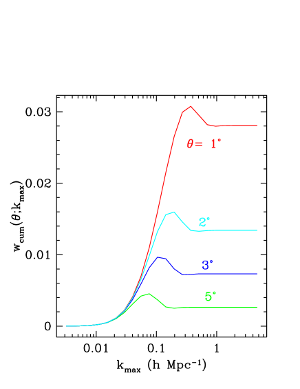
Figure 1: The cumulative value of the angular correlation function, considering all $k-$ modes up to $k_{\rm max}$. The response function is that for the APM survey, and the power spectrum used is the best-fit CDM-like power spectrum for that survey.

Inversion offers an excellent way out of this dilemma. Upon inverting, we will be using all the large scale information and throwing out all the small scale information. Mathematically, this is done in a trivial way:

• Perform the inversion and get $P$ and its associated error matrix $C_{P}$.

• Throw away all the small scale bins from step 1 by truncating $P$ and $C_{P}$. This is equivalent to marginalizing over these modes. That is, the resulting smaller error matrix has implicitly integrated over all possible values of $P$ on small scales. It is not contaminated at all by small scale information.

• Use these large scale modes to constrain theories.

We now proceed to outline the inversion process.

3 Inversion

One’s first thought upon encountering Eq.[1] is to simply invert the matrix $K$ to obtain a estimator for the power spectrum:

$$\hat{P}_{\alpha}=K^{-1}_{\alpha,i}\hat{w}_{i}$$ (2)

where the set of ${\hat{w}_{i}}$ are the estimators for the angular correlation function. This simple approach does not work. The inversion is very unstable and typically leads to nonsense. This is because the solution is degenerate (or $K$ is singular) as we typically want to obtain more information about $P(k)$ than available in $w(theta)$. In order to regulate the inversion, we need to introduce a bit of formalism.

We will assume that we are handed a set of $N_{w}$ estimators for the angular correlation function, ${\hat{w}_{i}}$, each $i$ corresponding to one of the $N_{w}$ angular bins. In addition, we assume we are handed the full error matrix for this set of estimators, $C_{w}$, an $N_{w}\times N_{w}$ matrix. This could be computed from first principles, or it could be estimated from a set of simulations. Mathematically, the simplest assumption is that the errors have a Gaussian distribution so that the probability that the angular correlation function is equal to ${w_{i}}$ is

$${\cal P}\left(\bigg{\{}w_{i}\bigg{\}}\right)\propto\exp\Big{\{}-{1\over 2}\left(w_{i}-\hat{w}_{i}\right)(C_{w}^{-1})_{ij}\left(w_{j}-\hat{w}_{j}\right)\Big{\}}$$ (3)

In order to invert, we need to assume more, we need to assume that the power spectrum is “smooth.” This assumption is put in by a second exponential in the probability distribution (Press et al. , 1992):

$${\cal P}\left(\bigg{\{}P_{\alpha}\bigg{\}}\right) \propto \exp\Big{\{}-{1\over 2}\left(K_{i\alpha}P_{\alpha}-\hat{w}_{i}\right)C^{-1}_{ij}\left(K_{j\beta}P_{\beta}-\hat{w}_{j}\right)\Big{\}}$$ (4)

$$\times \exp\Big{\{}-{\lambda\over 2}P_{\alpha}H_{\alpha\beta}P_{\beta}\Big{\}}$$ (5)

where now we have explicitly eliminated $w$ in favor of $P$ using Limber’s Equation. The second exponential here can be viewed as a prior distribution. It is implemented by putting in some matrix $H$ (see Press et al. 1992 for some examples) which makes it costly for $P$ to vary too much. Here we use for $H$ the first difference matrix, equation 18.5.3. in Press et al. (1986). We have tried other difference matrices with little effect on the results. For historical reasons, we have actually taken $kP(k)$ to be the unknown function. This means that we are smoothing $kP(k)$ to be locally flat.

This entire $H$ term is weighted by a free parameter $\lambda$, which allows one to tune the relative weights of the first and second exponential. One of the questions which will occupy us below is, What should $\lambda$ be set to? If one distrusts priors, $\lambda$ should be set very small to have little effect. This will have to be balanced by the requirement that the inversion is stable.

The argument of the exponential in Eq.[5] is quadratic in $P$. Thus it can be rewritten as

$${\cal P}\left(\bigg{\{}P_{\alpha}\bigg{\}}\right)\propto\exp\Big{\{}-{1\over 2}\left(P_{\alpha}-\hat{P}_{\alpha}\right)(C_{P}^{-1})_{\alpha\beta}\left(P_{\beta}-\hat{P}_{\beta}\right)\Big{\}}$$ (6)

where the estimator for the power spectrum is

$$\hat{P}_{\alpha}\equiv(C_{P}^{-1})_{\alpha\beta}(K^{t})_{\beta i}(C_{w}^{-1})_{ij}\hat{w}_{j}$$ (7)

and the error matrix is

$$C_{P,\alpha\beta}\equiv\left[(K^{t})_{\alpha i}(C_{w}^{-1})_{ij}K_{j\beta}+\lambda H_{\alpha\beta}\right]^{-1}.$$ (8)

Note that in the limit that $\lambda\rightarrow 0$ we do indeed recapture our initial guess, $\hat{P}=K^{-1}\hat{w}$. By varying $\lambda$ we can now move away from this unstable solution. Also note that while Press et al. (1992) refrain themselves from talking about the $\lambda PHP$ term as a prior, this interpretation is essential if we are to obtain an error matrix for $P$.

4 Tests of Inversion: Constraints on Cosmological Models

The simplest test of an inversion technique is to compare the recovered power spectrum with the true, underlying spectrum. There are several problems with this, though. First, and foremost, we do not know the true power spectrum. This difficulty can be surmounted by working with simulations, with which it is possible to generate angular catalogues. However, even if the true power spectrum is known, there is always the quantitative problem of determining how good the inversion is. This problem is exascerbated when the estimates of the power spectrum in adjacent bins are correlated. How do we make sense of the full error matrix for $P(k)$?

One way to test inversion is to put constraints on the parameters in a cosmological model. First, the constraints can be placed in the parameter space using the angular data, and then a second set of constraints can be drawn using the inferred power spectrum. These should agree. In fact, the method described in §2 is linear: the estimators for $P(k)$ are linear in the estimators of $w$. Really, then, the inversion process can be thought of as a new basis for the data, the “$P$” basis instead of the “$w$” basis. Through this prism, it is clear that the constraints on parameters should be independent of basis.

Figure 2: The angular correlation function from the APM survey (points with error bars). Also shown is the angular correlation function associated with the best fit CDM model from the contours in Figure 3.

For our example, we will choose the APM survey (Maddox et al. 1990), with data points and error bars shown in Figure 2. Errors are from the dispersion in 4 subsamples of the APM pixel maps (same as in Baugh & Efstathiou 1994) and are assumed to be diagonal. We have tried several ways of estimating the full covariance matrix for $w$. First, we have estimated it directly from the four quadrants of the APM survey. This produced a covariance matrix which was far too noisy. We then generated ten separate mock APM catalogues and estimated the covariance matrix from these forty sets ($10\times$ four quadrants for each). This proceedure worked on smaller angular scales but broke down on the largest scales (probably because the simulations were not large enough). One could also estimate $C_{w}$ analytically by assuming that the underlaying fluctuations are Gaussian. The results that we have obtained using the full covariance matrix of $C_{w}$, but with smaller angular scales (ie $\theta<10$ deg), give larger errors, but not much different in qualitative terms from the results that will be present here. This paper is mostly concerned with the inversion process for fixed ($w,C_{w}$) so we will simply assume here that $C_{w}$ is diagonal and leave off-diaginal errors for future work.

The model we choose to constrain is the CDM-like power spectrum with power spectrum

$$P(k)=AkT^{2}(k;\Gamma)$$ (9)

where $T$ is the BBKS (Bardeen, et al. 1986) transfer function. There are two free parameters in this model: the amplitude $A$ and the shape parameter $\Gamma$. We first determine the constraints on these parameters using the angular correlation data. Specifically, we calculate

$$\chi^{2}\equiv\sum_{i=1}^{N_{w}}{(w_{i}(\Gamma,A)-\hat{w}_{i})^{2}\over C_{w,ii}}$$ (10)

where we have explicitly indicated that $w_{i}$ depends on the parameters $(A,\Gamma)$ via Limber’s Equation Eq.[1]. Figure 3 shows the allowed one- and two- sigma regions in this parameter space. These contours will be our basis for judging the efficiency of the inversion. If we include all $k-$ modes, we should recover identical contours from the inverted spectrum. The main advantage of inversion is that once we have performed a successful inversion, we can throw out the small scale $k-$ modes and generate a new, more reliable allowed region.

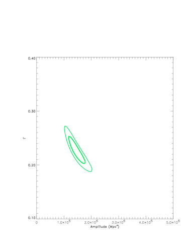
Figure 3: Allowed one- and two- sigma regions in CDM-like parameter space from APM survey. “Standard CDM” corresponds to $\Gamma=0.5$; COBE-normalization sets $A\simeq 10^{7}$ Mpc⁴.

5 Inversion of APM Correlation Function

We now test the inversion algorithm of §3 on the APM data. The extracted power is shown in Figure 4. The error bars are the square roots of the diagonal elements of $C_{P}$. For each bin, this error then includes the uncertainties induced by marginalizing over all other $k-$ modes. Also shown in Figure 4 is the power spectrum obtained by Lucy’s method (from Table 2 in Gaztañaga & Baugh 1998). These agree very well except on small scales. However, most of the disagreement is illusory because we are only using angular scales $\theta>0.5$ degree which has limited information about the power on scales $k>0.5{\rm Mpc}^{-1}$.

Figure 4: The power spectrum obtained by inverting the APM correlation function. Square symbols are from Bayesian inversion described in §3; circles are from Lucy’s method. The free parameter $\lambda$ in Eq.[5] has been set to an “intermediate” value here $10^{-4}$. The solid curve corresponds to the best-fit CDM like model.

Some of the disagreement between the two methods on small scales results from a more subtle effect. The estimates of the power spectrum on small scales are highly correlated, as shown in Figure 5. This means that the overall amplitude in any of these modes is uncertain This uncertainty is reflected in the large diagonal error bars. One can think of this in terms of linear combinations of the modes. One linear combination – the sum of power in the all the bins or the average power – is very uncertain. However, all other linear combinations – and therefore the shape – are known quite accurately.

Figure 5: The full covariance matrix of the power spectrum depicted in Figure 4. Each element is normalized by the diagonal: $C_{P,ij}/\sqrt{C_{P,ii}C_{P,jj}}$. Note the large covariances among bins $15-23$, corresponding to $k\ga 0.2h{\rm Mpc}^{-1}$.

We now test the inversion to see if it recaptures the constraints on the parameters $\Gamma$ and $A$ that were obtained in Figure 3 the angular correlation function itself. Figure 6 shows these two sets of contours; they agree extremely well, suggesting that the inversion has been successul.

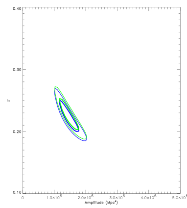
Figure 6: Allowed one- and two-sigma region in parameter space from APM using the angular correlation function directly and the extracted power spectrum with its error matrix $C_{P}$.

Finally, Figure 7 shows the contours one obtains by throwing out the small scale data ($k<=0.1h{\rm Mpc}^{-1}$). As one might expect, the allowed region gets much larger, but the qualitative statement that small $\Gamma\sim 0.25$ is preferred remains true. Gaztanaga & Baugh (1998) found a higher value of $\Gamma=0.45\pm 0.10$, over the four points in range $0.02<k<0.06h{\rm Mpc}^{-1}$. For this narrower range of scales our allowed region does indeed peak closer to $\Gamma=0.4$ as expected from the agreement in both $P(k)$ estimations shown in Figure 4.

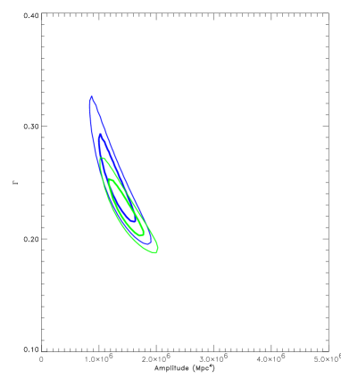
Figure 7: Same as Figure 6, except now only the large scale data has been used.

Figures 4-7 are for a particular value ($10^{-4}$) of the free parameter $\lambda$ which sets the importance of the smoothness prior in Eq.[5]. What motivates this choice and how do the results change as $\lambda$ gets bigger or smaller?

First consider reducing $\lambda$ thereby trying to eliminate the dependence on the smoothing prior. Figure 8 shows the inferred power spectrum in this case. Although the mean $P(k)$ agrees with that using a stronger smoothness prior, the error bars are significantly larger. The larger errors result from the fact that the power spectrum estimates are much more highly correlated if the prior is weak, due to the degeneracy in the inverse problem solution. To understand this, consider the limit of no smoothness prior. In that case, it is possible to fit the $w(\theta)$ data with an extremely choppy power spectrum. One bin might have huge power, while another has negative power. This choppiness is evident on large scales in Figure 8. One could still try to use such a choppy power spectrum to fit models. But the results in each bin do not make much sense by themselves and there are large covariances among the different bins. So this is not a very useful representation of the data. The large correlations between different bins also affects the constraints on CDM models, which use only the large scale data. This is shown in Figure 9. The small $\lambda$ constraints (weak prior) are much less restrictive than the stronger prior. This reflects the fact that the large scale estimates are highly dependent on the small scale estimates. Hence, marginalizing over the latter leads to constraints which are not very tight. Incidentally, the constraints obtained using all the data are identical to the constraints coming from $w(\theta)$ itself (the analogue of Figure 6). So the inversion is accurate, but not useful because the modes are so correlated.

Figure 8: The inverted power spectrum using a weak smoothness prior ($\lambda=10^{-5}$; squares) and the moderate prior ($\lambda=10^{-4}$; circles) used previously. The larger error bars in the weak prior case result from higher bin-to-bin correlations.

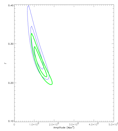
Figure 9: Constraints on parameter space using only large scale data from moderate prior (thick lines) and weak prior (thin lines). The weak prior leads to less restrictive constraints.

Introducing a stronger prior leads to an inaccurate power spectrum extraction. The prior is given too much weight, and the data loses out. We can see this in Figure 10, which shows the power spectrum using a strong prior as opposed to the moderate one advocated earlier. At intermediate scales the power estimates differ decidedly. Examining the constraints on the cosmological parameters illustrates that the incorrect inversion is the one using the strong prior. Figure 11 shows that the strong prior leads to incorrect constraints. The information in the data has not been processed accurately.

Figure 10: The inverted power spectrum using a strong smoothness prior ($\lambda=10^{-3}$; squares) and the moderate prior ($\lambda=10^{-4}$; circles) used previously. The strong prior leads to an incorrect determination of the power on intermediate scales.

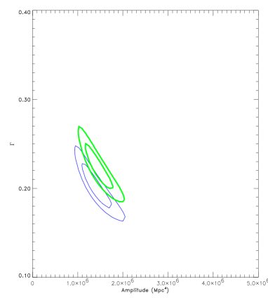
Figure 11: Constraints on parameter space using all the data from moderate prior (thick lines) and strong prior (thin lines). The strong prior leads to incorrect constraints, while the moderate prior reconstructs perfectly the constraints obtained from $w(\theta)$ directly.

6 Conclusions

Very valuable information is contained in the angular correlation function. A useful way to extract this information is to invert it and obtain an estimator for the three dimensional power spectrum. We have introduced here a method that is different from the one used previously and have focused intensely on its advantages and its features. However, it is important not to lose sight of the fact that this inversion technique agrees extremely well with Lucy’s method, the previous inversion tool. This agreement suggests that we (as a community) are correctly inferring the power spectrum from the angular correlation function.

We worked with the angular APM data; our results for the three dimensional power spectrum and its error matrix are shown in Figures 4 and 5. Files containing these numbers are available at http://www-astro-theory.fnal.gov/Personal/dodelson/Inversion/power.html.

Having reiterated these successes, we warn that there are a number of issues not explored here that warrant further study:

• The distribution for the angular correlation function is not Gaussian, as assumed in Eq.[3]. Indeed, even if the fluctuations are Gaussian – as they are predicted to be in inflationary models on large scales but are certainyl not on small scales – the likelihood function is not Gaussian in $w$. The full likelihood function is hopelessly complicated (Dodelson, Hui & Jaffe, 1997), but perhaps there are approximations that can be made which account for the non-Gaussianity. Indeed, there has recently been some progress along these lines (Meiksin & White, 1999; Scoccimarro, Zaldarriaga & Hui, 1999; Hamilton, 1999; Hamilton & Tegmark, 1999).

• In performing the inversion, we assumed that the power spectrum was separable: $P(k,t)=P(k)f(t)$ and assumed a simple form for $f(t)$ ( $f=a^{\beta}$). Similarly, we have not explored at all the uncertainties in the selection function. We have also used the small angle approximation. All of these fold into the kernel in Limber’s Equation Eq.[1]. They may be sufficient for APM (e.g. see Gaztañaga & Baugh, 1998), but need to be revisited for deeper surveys, such as the Sloan Digital Sky Survey.

• We assumed that the covariance matrix for the angular correlation function is diagonal. The exact nature of this matrix depends on the binning proceedure, but clearly it is not diagonal. Our efforts to obtain the full covariance matrix from simulations failed, but perhaps simulations on small scales could be supplemented by linear calculations on large scales to obtain the full covariance matrix.

• Related to the first and third points is our assumption that the covariance matrix $C_{w}$ does not depend on $w$ itself. This again is not true and needs to be accounted for when constraining parameters in a cosmological model.

• Although we explored the consequences of varying the smoothness prior, we did not explore how these variations couple to: (i) different binning schemes for $w(\theta)$; (ii) different binning schemes for $P(k)$; or (iii) theoretical models which vary more rapidly than the ones discussed here (e.g. high baryon models retain signatures of primordial acoustic oscillations).

All of these assumptions were implicit in previous inversions, and other ways of obtaining the power spectrum involve a similar number of assumptions. So measuring the angular correlation function still is an excellent way to get at the power spectrum. Clearly, though, more work is needed to enable the extraction to be as powerful and accurate as possible.

Acknowledgments We thank Carlton Baugh for helpful comments. We thank the referee for his inciteful comments. His careful reading of the manuscript has really helped us improve the text. We are especially grateful to him for taking the time to work through our arguments, and for spotting some of the weaknesses in them. We acknowledge support from NATO Collaborative Research Grants Programme CRG970144. SD is supported by NASA Grant NAG 5-7092 and the DOE. EG acknowledges support by spanish DGES(MEC), project PB96-0925.

7 References

Baugh, C.M., Efstathiou, G., 1993, MNRAS 265, 145

Baugh, C.M., Efstathiou, G., 1994, MNRAS 267, 323

Bardeen, J. M., Bond, J. R., Kaiser, N., & Szalay, A. S., 1986, ApJ , 304, 15

Bond, J.R., Jaffe, A. H., & Knox, L., 1998, Phys ReV D, 57, 2117

Collins, C. A. Nichol, R. C., & Lumsden, S. L. 1992, MNRAS , 254, 295

Dodelson, S., Hui, L., Jaffe, A. H., 1997, astro-ph/9712074

Gaztañaga, E. & Baugh, C.M., 1998, MNRAS , 294, 229

Hamilton, A.J.S., 1999, astro-ph/9905191

Hamilton, A.J.S. & Tegmark, M., 1999, astro-ph/9905192

Maddox, S. J., Efstathiou, G., Sutherland, W. J., & Loveday, L. 1990, MNRAS , 242, 43P

Meiksin, A. & White, M., 1998, astro-ph/9812129

Press, W.H., Teukolsky, S.A., Vetterling, W.T., & Flannery, B.P., 1992, Numerical Recipes (Cambridge)

Scoccimarro, R., Zaldarriaga, M. & Hui, L., 1999, astro-ph/9901099