Measuring the equation of state of the intergalactic medium

Abstract

Numerical simulations indicate that the smooth, photoionized intergalactic medium (IGM) responsible for the low column density Ly$\alpha$ forest follows a well defined temperature-density relation, which is well described by a power-law $T=T_{0}(\rho/\bar{\rho})^{\gamma-1}$. We demonstrate that such an equation of state results in a power-law cutoff in the distribution of line widths ($b$-parameters) as a function of column density ($N$) for the low column density ($N\la 10^{14.5}\,\rm cm^{-2}$) absorption lines. This explains the existence of the lower envelope which is clearly seen in scatter plots of the $b(N)$-distribution in observed QSO spectra. Even a strict power-law equation of state will not result in an absolute cutoff because of line blending and contamination by unidentified metal lines. We develop an algorithm to determine the cutoff, which is insensitive to these narrow lines. We show that the parameters of the cutoff in the $b(N)$-distribution are strongly correlated with the parameters of the underlying equation of state. We use simulations to determine these relations, which can then be applied to the observed cutoff in the $b(N)$-distribution to measure the equation of state of the IGM. We show that systematics which change the $b(N)$-distribution, such as cosmology (for a fixed equation of state), peculiar velocities, the intensity of the ionizing background radiation and variations in the signal to noise ratio do not affect the measured cutoff. We argue that physical processes that have not been incorporated in the simulations, e.g. feedback from star formation, are unlikely to affect the results. Using Monte Carlo simulations of Keck spectra at $z=3$, we show that determining the slope of the equation of state will be difficult, but that the amplitude can be determined to within ten per cent, even from a single QSO spectrum. Measuring the evolution of the equation of state with redshift will allow us to put tight constraints on the reionization history of the universe.

1 INTRODUCTION

The intergalactic medium (IGM) at high redshift ($z\sim 2$–5) manifests itself observationally by absorbing light from distant quasars. Resonant Ly$\alpha$ absorption by neutral hydrogen along the line of sight to a quasar results in a fluctuating Ly$\alpha$ transmission (optical depth). Regions of enhanced density give rise to increased absorption and appear as a forest of absorption lines bluewards of the quasar’s Ly$\alpha$ emission line. The fact that not all the light is absorbed implies that the IGM is highly ionized [Gunn & Peterson 1965], but the time and origin of the reionization of the gas are still unknown. Since quasars and young stars are sources of ionizing radiation, the ionization history of the gas depends on the evolution of the quasar population and the star formation history of the universe.

Hydrodynamical simulations of structure formation in a universe dominated by cold dark matter and including an ionizing background, have been very successful in explaining the properties of the Ly$\alpha$ forest [e.g. Cen et al. 1994, Zhang, Anninos & Norman 1995, Hernquist et al. 1996, Miralda-Escudé et al. 1996, Theuns, Leonard & Efstathiou 1998, Theuns et al. 1998, Davé et al. 1999]. They show that the low column density ($N\la 10^{14.5}\,\rm cm^{-2}$) absorption lines arise in a smoothly varying low-density ($\delta\la 10$) IGM. Since the overdensity is only mildly non-linear, the physical processes governing this medium are well understood and relatively easy to model. On large scales the dynamics are determined by gravity, while on small scales gas pressure is important. The existence of a simple physical framework and the abundance of superb observational data make the Ly$\alpha$ forest an extremely promising cosmological laboratory (see Rauch [Rauch 1998] for a review). In this paper, we shall investigate the effect of the thermal state of the IGM on the forest.

For the low-density gas responsible for the Ly$\alpha$ forest, shock heating is not important and the gas follows a well defined temperature-density relation. The competition between photoionization heating and adiabatic cooling results in a power-law ‘equation of state’ $T=T_{0}(\rho/\bar{\rho})^{\gamma-1}$ [Hui & Gnedin 1997]. This equation of state depends on cosmology and reionization history. For models with abrupt reionization, the IGM becomes nearly isothermal ($\gamma\approx 1$) at the redshift of reionization. After reionization, the temperature at the mean density ($T_{0}$) decreases while the slope ($\gamma-1$) increases because higher density regions undergo less expansion and increased photoheating. Eventually, when photoheating balances adiabatic cooling as the universe expands, the imprints of the reionization history are washed out and the equation of state approaches an asymptotic state, $\gamma=1.62$, $T_{0}\propto\left[\Omega_{b}h^{2}/\sqrt{\Omega_{m}h^{2}}\right]^{1/1.7}$ [Hui & Gnedin 1997]. Since the reionization history of the universe is still unknown, the physically reasonable ranges for the parameters of the equation of state are very large ($10^{3.0}\,\rm K<T_{0}<10^{4.5}\,K$ and $1.2<\gamma<1.7$ [Hui, Gnedin & Zhang 1997, Hui & Gnedin 1997]).

The smoothly varying IGM gives rise to a fluctuating optical depth in redshift space. Many of the optical depth maxima can be fitted quite accurately with Voigt profiles. The distribution of line widths depends on the initial power spectrum, the peculiar velocity gradients around the density peaks and on the temperature of the IGM. However, there is a lower limit to how narrow the absorption lines can be. Indeed, the optical depth will be smoothed on a scale determined by three processes [Hui & Rutledge 1997]: thermal broadening, baryon (Jeans) smoothing and possibly instrumental, or in the case of simulations, numerical resolution. The first two depend on the thermal state of the gas. While for high-resolution observations (echelle spectroscopy) the effective smoothing scale is not determined by the instrumental resolution, numerical resolution has in fact been the limiting factor in many simulations (see Theuns et al. [Theuns et al. 1998] for a discussion).

The distribution of line widths is generally expressed as the distribution of the widths of Voigt profile fits to the absorption lines, the $b$-parameters. While the first numerical simulations showed good agreement with the observed $b$-parameter distribution, higher resolution simulations of the standard cold dark matter model produced a larger fraction of narrow lines than observed [Theuns et al. 1998, Bryan et al. 1998]. Theuns et al. [Theuns et al. 1998] suggested that an increase in the temperature of the IGM might broaden the absorption lines, while Bryan et al. [Bryan et al. 1998] argued that the most natural way to broaden the lines is to change the density distribution directly. Note that increasing the temperature will also change the density distribution of the gas through increased baryon smoothing (Theuns, Schaye & Haehnelt 1999).

Theuns et al. [Theuns et al. 1999a] showed that changing the cosmology (lowering $\Omega_{m}$ from 1.0 to 0.3 and doubling $\Omega_{b}h^{2}$ to 0.025) significantly broadens the absorption lines, although some discrepancy with observations may remain. One way to increase the temperature further would be to change the reionization history. Uncertainties in the redshift of He reionization, in particular, can affect the temperature of the IGM. Haehnelt & Steinmetz [Haehnelt & Steinmetz 1998] demonstrated that different reionization histories result in observable differences in the $b$-distribution. Other mechanisms that have been proposed to boost the temperature are photoelectric heating of dust grains  [Nath, Sethi & Shchekinov 1999], Compton heating by the hard X-ray background [Madau & Efstathiou 1999] and radiative transfer effects associated with the ionization of He ii by QSOs in the optically thick limit [Abel & Haehnelt 1999].

Unfortunately, the $b$-distribution is not very well suited for investigating the thermal state of the IGM. Although some of the broad lines correspond to density fluctuations on scales that are affected, among other things, by thermal smoothing [Theuns et al. 1999b], many are caused by heavy line blending and continuum fitting errors. The cutoff in the $b$-distribution, on the other hand, will depend mainly on the temperature of the IGM and is therefore potentially a powerful statistic. In practice its usefulness is limited because many narrow lines occur in the wings of broader lines. Such narrow lines are often introduced by numerical Voigt profile fitting algorithms (such as VPFIT [Carswell et al. 1987]) to improve the quality of the overall fit to the quasar spectrum. If the physical structure responsible for the absorption does not consist of discrete clouds, then the widths of these blended lines will have no relation to the thermal state of the gas. Furthermore, the number and widths of these narrow blended lines depend on the Voigt profile fitting algorithm that is used and on the signal to noise of the quasar spectrum.

The $b$-parameter distribution is usually integrated over a certain column density range. Since the $b$-distribution might depend on column density ($N$), more information is contained in the full $b(N)$-distribution. Scatter plots of the $b(N)$-distribution have been published for many observed QSO spectra [e.g. Hu et al. 1995, Lu et al. 1996, Kirkman & Tytler 1997, Kim et al. 1997]. These plots show a clear cutoff at low $b$-parameters. However, this cutoff is not absolute. There are some narrow lines, especially at low column densities. Lu et al. [Lu et al. 1996] and Kirkman & Tytler [Kirkman & Tytler 1997] use Monte Carlo simulations to show that many of these lines are caused by line blending and noise in the data. Some contamination from unidentified metal lines is also expected.

The cutoff in the $b(N)$-distribution increases slightly with column density. Hu et al. [e.g. Hu et al. 1995] conclude from Monte Carlo simulations that this correlation is primarily an artifact of the much larger number of lines at lower column density and the increased scatter in the $b$-determinations. Kirkman & Tytler [Kirkman & Tytler 1997] however, conclude from similar simulations that the correlation between the lowest $b$-values and column density is a real physical effect. (Note that this correlation is different from the one reported by Pettini et al. [Pettini et al. 1990]. They found a general correlation between the $b$-parameter and column density of all lines. This correlation was later shown to be an artifact of the line selection and fitting procedure [Rauch et al. 1993].) A lower envelope which increases with column density has also been seen in numerical simulations [Zhang et al. 1997].

In this paper we shall demonstrate that the cutoff in the $b(N)$-distribution is determined by the equation of state of the low-density gas. Furthermore, we shall show that the cutoff can be determined robustly and is unaffected by systematics like changes in cosmology (for a fixed equation of state) and can therefore be used to measure the equation of state of the IGM.

We test our methods using smoothed-particle hydrodynamic (SPH) simulations of the Ly$\alpha$ forest as described by Theuns et al. [Theuns et al. 1998, Theuns et al. 1999a]. The parameters of the simulations are summarised in section 2. The relation between the $b(N)$-cutoff and the equation of state is investigated in section 3, which forms the heart of the paper. Section 4 contains a detailed description of the procedure used to fit the cutoff in simulated Keck spectra. Systematic effects are discussed in section 5. In section 6 we test the procedure using Monte Carlo simulations. Finally, we summarise and discuss the main results in section 7.

2 SIMULATIONS

We have simulated six different cosmological models, characterised by their total matter density $\Omega_{m}$, the value of the cosmological constant $\Omega_{\Lambda}$, the rms of mass fluctuations in spheres of radius 8$h^{-1}$ Mpc, $\sigma_{8}$, the baryon density $\Omega_{b}h^{2}$ and the present day value of the Hubble constant, $H_{0}\equiv 100h~{}{\rm km}\,{\rm s}^{-1}\,{\rm Mpc}^{-1}$. The parameters of these models are summarised in Table 1. In addition to these models, we simulated a model that has the same parameters as model Ob, but with the He i and He ii heating rates artificially doubled. This may provide a qualitative model of the heating due to radiative transfer effects during the reionization of helium [Abel & Haehnelt 1999]. We will call this model Ob-hot. The amplitude of the initial power spectrum is normalised to the observed abundance of galaxy clusters at $z=0$, using the fits computed by Eke, Cole & Frenk [Eke, Cole & Frenk 1996]. We model the evolution of a periodic, cubic region of the universe of comoving size $2.5h^{-1}$ Mpc.

Table 1: Models simulated

Model	$\Omega_{m}$	$\Omega_{\Lambda}$	$\Omega_{b}h^{2}$	$h$	$\Gamma_{\hbox{H\,{\sc i}}}$
S	1	0	0.0125	0.5	HM/2
Sb	1	0	0.025	0.5	HM
O	0.3	0	0.0125	0.65	HM/2
Ob	0.3	0	0.025	0.65	HM
L	0.3	0.7	0.0125	0.65	HM/2
Lb	0.3	0.7	0.025	0.65	HM

The code used is adapted from the HYDRA code of Couchman et al. [Couchman, Thomas & Pearce 1995], which uses smooth particle hydrodynamics (SPH) [Lucy 1970, Gingold & Monaghan 1977]; see Theuns et al. [Theuns et al. 1999a, Theuns et al. 1998] for details. These simulations use $64^{3}$ particles of each species, so the SPH particle masses are $1.65\times 10^{6}\,(\Omega_{b}h^{2}/0.0125)(h/0.5)^{-3}{\rm M}_{\odot}$ and the CDM particles are more massive by a factor $\Omega_{\rm CDM}/\Omega_{b}$. This resolution is sufficient to simulate line widths reliably [Theuns et al. 1998, Bryan et al. 1998, note that in the hotter simulations numerical convergence will be even better than in the cooler model S, which was investigated in detail by Theuns et al. [Theuns et al. 1998]].

We assume that the IGM is ionized and photoheated by an imposed uniform background of UV-photons that originates from quasars, as computed by Haardt & Madau [Haardt & Madau 1996]. This flux is redshift dependent, due to the evolution of the quasar luminosity function. The amplitude of the flux is indicated as ‘HM’ in the $\Gamma_{\hbox{H\,{\sc i}}}$ column of Table 1 (where $\Gamma_{\hbox{H\,{\sc i}}}$ is the H i ionization rate due to the ionizing background). For the low $\Omega_{b}h^{2}$ models, we have divided the ionizing flux by two, indicated as ‘HM/2’. We do not impose thermal equilibrium but solve the rate equations to track the abundances of H i, H ii and He i, He ii and He iii. We assume a helium abundance of $Y=0.24$ by mass. See Theuns et al. [Theuns et al. 1998] for further details.

At several output times we compute simulated spectra along 1200 random lines of sight through the simulation box. Each spectrum is convolved with a Gaussian with full width at half maximum of FWHM = 8 ${\rm km}\,{\rm s}^{-1}$, then resampled onto pixels of width 3 ${\rm km}\,{\rm s}^{-1}$ to mimic the instrumental profile and characteristics of the HIRES spectrograph on the Keck telescope. We rescale the background flux in the analysis stage such that the mean effective optical depth at a given redshift in all models is the same as for the Ob model. This model has a mean absorption in good agreement with observations [Rauch et al. 1997] (Ob has $\bar{\tau}_{\rm eff}=0.93$, 0.33 and 0.14 at $z=4$, 3 and 2). Finally, we add to the flux in every pixel a Gaussian random signal with zero mean and standard deviation $\sigma=0.02$ to mimic noise. The spectra cover a small enough velocity range to be fit by a flat continuum, as chosen by a simple procedure [Theuns et al. 1998] described as follows. A low average continuum is assumed initially, then all pixels below and not within 1 $\sigma$ of this level are rejected and a new average flux level for the remaining pixels is computed. The last two steps are repeated until the average flux varies by less than 1%. This final average flux level is adopted as the fitted continuum and the spectrum is renormalised accordingly. The absorption features in these mock observations are then fitted with Voigt profiles using an automated version of VPFIT [Carswell et al. 1987].

Although the simulated models have different equations of state, they cover only a limited part of the possible parameter space $(T_{0},\gamma)$. The models were originally intended to investigate the dependence of QSO absorption line statistics on cosmology [Theuns et al. 1999a]. Changing the reionization history can lead to very different values of $T_{0}$ and $\gamma$. To quantify the relation between the cutoff in the $b(N)$-distribution and the equation of state, it is necessary to include models covering a wide range of $T_{0}$ and $\gamma$. We therefore created models with particular values of $T_{0}$ and $\gamma$ by imposing an equation of state on model Ob. This was done by moving the SPH particles in the temperature-density plane. The new models have the same three components (low- and high-density power-law equations of state and shocked gas) as the original model, but a different equation of state for the low-density gas. In particular, the intrinsic scatter around the power-law is left unchanged.

3 THE $\mn@boldsymbol{b(N)}$-CUTOFF AND THE EQUATION OF STATE

Fig. 1 shows a contour plot of the mass-weighted distribution of fluid elements (SPH particles) from a numerical simulation in the temperature-density diagram. Noting that the number density of fluid elements increases by an order of magnitude with each contour level, it is clear that the vast majority of the low-density gas ($\rho_{b}/\bar{\rho}_{b}\la 10$) follows a power-law equation of state (dashed line). The two other components visible in Fig. 1 are hot, shocked gas which cannot cool within a Hubble time and colder, high-density gas for which H i and He ii line cooling is effective.

Figure 1: The mass-weighted distribution of fluid elements (SPH particles) in the temperature-density plane for model Ob-hot at $z=3$. Three contour levels are plotted. The number density of fluid elements increases by an order of magnitude with each contour level. The dashed line is a power-law (least absolute deviation) fit to the temperature-density relation of the gas with density in the range $-0.7\leq\log(\rho_{b}/\bar{\rho}_{b})\leq 0.3$. Clearly, the vast majority of the low-density gas follows this tight temperature-density relation. The dotted line shows the result of a similar fit for model S.

In Fig. 2a we plot the $b(N)$-distribution for 800 random absorption lines taken from the spectra of model Ob-hot at redshift $z=3$. A cutoff at low $b$-values, which increases with column density, can clearly be seen. In Fig. 2b only those lines for which VPFIT gives formal errors in both $b$ and $N$ that are smaller than 50 per cent are plotted. This excludes most of the lines that have column density $N\la 10^{12.5}\,\rm cm^{-2}$ as well as many of the very narrow lines below the cutoff. Although the formal errors of the Voigt profile fit given by VPFIT have only limited physical significance, lines in blends tend to have large errors. Since the $b$-parameters for blended lines can have values smaller than the minimum set by the thermal smoothing scale (i.e. thermal broadening and baryon smoothing), these lines will tend to smooth out any intrinsic cutoff. Removing the lines with the largest relative errors therefore results in a sharper cutoff. A smaller maximum allowed error would result in the removal of many of the regular, isolated lines.

Figure 2: The $b(N)$-distribution for 800 random lines from model Ob-hot (a,b) and S (c), at $z=3$. The position of each line is indicated by a cross. Errors are not displayed. In panels (b) and (c) only those lines are plotted for which VPFIT gives formal errors $\Delta b/b<0.5$, $\Delta N/N<0.5$. The dashed line is the cutoff for the lines plotted in panel (b) over the range $10^{12.5}\,\rm cm^{-2}\leq N\leq 10^{14.5}\,\rm cm^{-2}$. Removing the lines with the largest relative errors in the Voigt profile parameters sharpens the cutoff. The $b(N)$-distribution of the colder model S clearly cuts off at lower $b$-parameters than the $b(N)$-distribution of model Ob-hot.

The large number of data points plotted in Fig. 2a excludes the possibility that the slope in the cutoff is due to the large decrease in the number of lines with column density or the increase in scatter with decreasing column density (Hu et al. [e.g. Hu et al. 1995] reached this conclusion from analysing spectra that had about 250 absorption lines each).

The $b(N)$-distribution for the colder model S is plotted in Fig. 2c. Clearly, the distribution cuts off at lower $b$-values. Let us assume that the absence of lines with low $b$-values is due to the fact that there is a minimum line width set by the thermal state of the gas through the thermal broadening and/or baryon smoothing scales. Since the temperature of the low-density gas responsible for the Ly$\alpha$ forest increases with density (Fig. 1), we expect the minimum $b$-value to increase with column density, provided that the column density correlates with the density of the absorber.

To see whether this picture is correct, we need to investigate the relation between the Voigt profile parameters $N$ and $b$, and the density and temperature of the absorbing gas respectively. Peculiar velocities and thermal broadening make it difficult to identify the gas contributing to the optical depth at a particular point in redshift space. Furthermore, the centre of the Voigt profile fit to an absorption line will often be offset from the point where the optical depth is maximum. We therefore need to define a temperature and a density which are smooth and take redshift space distortions into account. We choose to use optical depth weighted quantities: the density of a pixel in velocity space is the sum, weighted by optical depth, of the density at all the pixels in real space that contribute to the optical depth of that pixel in velocity space. We then define the density corresponding to an absorption line to be the optical depth weighted density at the line centre. The temperature corresponding to absorption lines is defined similarly.

In Fig. 3 the optical depth weighted density and temperature are plotted for two random lines of sight (dashed lines in the middle two panels), as well as the flux (without noise), and real space density, temperature and peculiar velocity. The dashed curves in the top panels are the Voigt profiles fitted by VPFIT, vertical lines indicate the line centres. Absorption lines correspond to peaks in the (optically depth weighted) density and temperature, which are strongly correlated. Although the blends indicated by arrows can be traced back to substructure in the peaks, their profiles are mainly determined by the density and temperature of the gas in the main peaks.

Figure 3: Two random lines of sight through the box of model Ob-hot at $z=3$. From top to bottom the solid curves are the flux, gas density, temperature and peculiar velocity respectively, all as a function of Hubble velocity. The dashed curves in the top panel are the Voigt profiles fitted by VPFIT, vertical lines indicate the line centres. The arrows point at the line centres of lines with a $b$-parameter smaller than the cutoff value of the Hui-Rutledge formula (equation 10). These lines have column densities $N=10^{12.7}\,\rm cm^{-2}$ (left panel) and $N=10^{12.9}\,\rm cm^{-2}$ (right panel), and $b$-parameters 13.1 ${\rm km}\,{\rm s}^{-1}$ (left panel) and 13.6 ${\rm km}\,{\rm s}^{-1}$ (right panel). They appear as diamonds in Fig. 6. The dashed curves in the second and third panels are the optical depth weighted density and temperature respectively.

In Fig. 4 the optical depth weighted gas density is plotted as a function of column density for the absorption lines plotted in Fig. 2b. There exists a tight correlation between these two quantities. Note that lines with column densities $\la 10^{13}\,\rm cm^{-2}$ correspond to local maxima in underdense regions.

Figure 4: The optical depth weighted gas density at the line centres as a function of neutral hydrogen column density. Data points correspond to the lines plotted in Fig. 2b. The column density of a Voigt profile fit to an absorption line is strongly correlated with the density of the absorbing gas. The outlier at $\log(\rho/\bar{\rho_{b}})=2.50$ corresponds to a line in the wing of a highly saturated line.

The optical depth weighted temperature is plotted against the $b$-parameter in Fig. 5a. The result is a scatter plot with no apparent correlation. This is not surprising since many absorbers will be intrinsically broader than the local thermal broadening scale. In order to test whether the cutoff in the $b(N)$-distribution is a consequence of the existence of a minimum line width set by the thermal state of the gas, we need to look for a correlation between the temperature and $b$-parameters of the lines near the cutoff.

Determining a cutoff in an objective manner is nontrivial because of the existence of unphysically narrow lines in blends. We developed a fitting algorithm that is insensitive to these lines. This algorithm is described in the next section. Fig. 6 is a scatter plot of the lines with column density in the range $10^{12.5}\,\rm cm^{-2}\leq N\leq 10^{14.5}\,\rm cm^{-2}$. The cutoff fitted to this distribution is also shown (solid line). The lines that are used in the final iteration of the fitting algorithm, i.e. lines that are close to the solid line in Fig. 6, do indeed display a tight correlation between the temperature and $b$-parameter (Fig. 5b). The dashed line in Fig. 5b corresponds to the thermal width, $b=(2k_{B}T/m_{p})^{1/2}$, where $m_{p}$ is the mass of a proton and $k_{B}$ is the Boltzmann constant. Lines corresponding to density peaks whose width in velocity space is much smaller than the thermal width, have Voigt profiles with this $b$-parameter. Since the temperature plotted in Fig. 5 is the smooth, optical depth weighted temperature, we do not expect the relation between $T$ and $b$ to be identical to the one indicated by the dashed line, even if all the line widths were purely thermal. Although other definitions of the density and temperature are possible and will give slightly different results, qualitatively the results will be the same for any sensible definition of these physical quantities. Figs. 4 and 5b therefore suggest that the cutoff in the $b(N)$-distribution should be strongly correlated with the equation of state of the absorbing gas.

Figure 5: The optical depth weighted temperature at the line centres as a function of $b$-parameter. The left panel contains all lines plotted in Fig. 2b. In the right panel only those lines are plotted which have $b$-parameters within one mean absolute deviation of the power-law fit to the $b(N)$-cutoff plotted as the solid line in Fig. 6. Only for the lines near the cutoff are the $b$-parameters correlated with the temperature of the absorbing gas. The dashed line corresponds to the thermal width, $b=(2k_{B}T/m_{p})^{1/2}$.

Figure 6: The $b(N)$-distribution for those lines from Fig. 2b that have column densities in the range $10^{12.5}\,\rm cm^{-2}\leq N\leq 10^{14.5}\,\rm cm^{-2}$. The solid line is the fitted cutoff for this set of lines, the dot-dashed line is the cutoff for the colder model S. The horizontal dashed line indicates the minimum $b$-value of lines used in the fit, lines with smaller $b$-parameters are indicated by diamonds. This minimum $b$-value corresponds to the cutoff of the best-fitting Hui-Rutledge function (see section 4).

Let us look in more detail at the relation between the $b(N)$-cutoff and the equation of state. We have already shown (Fig. 1) that almost all the low-density gas follows a power-law equation of state:

$$\log(T)=\log(T_{0})+(\gamma-1)\log(\rho/\bar{\rho}).$$ (1)

The relations between the density/temperature and column density/$b$-parameter of the absorption lines near the cutoff can also be fitted by power-laws (Fig. 4 and Fig. 5b):

$$\log(\rho/\bar{\rho})=A+B\log(N/N_{0}),$$ (2)

$$\log(T)=C+D\log(b).$$ (3)

Combining these equations, we find that the $b(N)$-cutoff is also a power-law,

$$\log(b)=\log(b_{0})+(\Gamma-1)\log(N/N_{0}),$$ (4)

whose coefficients are given by,

$$\log(b_{0})={1\over D}\left[\log(T_{0})-C+(\gamma-1)A\right],$$ (5)

$$\Gamma-1={B\over D}(\gamma-1).$$ (6)

Hence the intercept of the cutoff, $\log b_{0}$, depends on both the amplitude and the slope of the equation of state, while the slope of the cutoff, $\Gamma-1$, is proportional to the slope of the equation of state. If we set $N_{0}$ equal to the column density corresponding to the mean gas density, then the coefficient $A$ vanishes and $\log b_{0}$ no longer depends on $\gamma$.

The cutoff in the $b(N)$-distribution is measured over a certain column density range. We choose to measure the cutoff over the interval $10^{12.5}\,\rm cm^{-2}\leq N\leq 10^{14.5}\,\rm cm^{-2}$. This interval corresponds roughly to the gas density range for which the equation of state is well fitted by a power-law. For lines with column density $N\la 10^{12.5}\,\rm cm^{-2}$, the scatter in the observations becomes very large due to noise and line blending. The relation between the gas overdensity and H i column density depends on redshift. Hence different column density intervals should be used for different redshifts if one wants to compare the equation of state for the same density range.

Fitting a cutoff to a finite number of lines introduces statistical uncertainty in the measured coefficients. We minimize the correlation between the errors in the coefficients by subtracting the average abscissa value (i.e. $\log N$) before fitting the cutoff. This can be done by setting $\log N_{0}$ in equation 4 equal to the mean $\log N$ of the lines in the column density range over which the cutoff is measured. This column density does in general not correspond to the mean gas density and hence $\log b_{0}$ will in general depend on $\gamma$. We will show below that this dependence can be removed by renormalising the equation of state.

In Fig. 7 we plot the temperature at mean density predicted from the power-law model (equation 5) as a function of the true $T_{0}$. Data points are determined by fitting power-laws to 500 sets of 300 random absorption lines. Error bars enclose 68 per cent confidence intervals around the medians. Solid circles are used for data from simulated models, open squares are used for models created by imposing an equation of state on model Ob. These conventions will be used throughout the paper. Fig. 8 is a similar plot for the slope of the equation of state (equation 6). The predicted and true parameters of the equation of state are highly correlated. The slight offset between the predicted and true quantities simply reflects the fact that the optical depth weighted density and temperature are not exactly the same as the true density and temperature of the absorbing gas (i.e. the $T$ and $\rho$ appearing in equation 1 are not exactly the same as those appearing in equations 2 and 3). The main conclusion to draw from these plots is that the power-law model works and that we can therefore use these equations to gain insight in the relationship between the equation of state and the cutoff in the $b(N)$-distribution.

Figure 7: The temperature at mean density predicted from the power-law model (equation 5) as a function of the true temperature at redshift $z=3$. Error bars enclose 68% confidence intervals around the medians, as determined from 500 sets of 300 random lines. Open squares indicate that the points resulted from imposing an equation of state with the given $T_{0}$ on model Ob. All points have similar values of $\gamma$. The dashed line is the least-squares fit.

Figure 8: The index $\gamma$ predicted from the power-law model (equation 6) as a function of the true index of the power-law equation of state at redshift $z=3$. Error bars enclose 68% confidence intervals around the medians, as determined from 500 sets of 300 random lines. Open squares indicate that the points resulted from imposing an equation of state with the given $\gamma$ on model Ob, while leaving $T_{0}$ unchanged. The dashed line is the least-squares fit.

The objective is to establish the relations between the cutoff parameters and the equation of state using simulations. These relations can then be used to measure the equation of state of the IGM using the observed cutoff in the $b(N)$-distribution. The amplitudes of the power-law fits to the cutoff and the equation of state are plotted against each other in Fig. 9. The relation between $\log b_{0}$ and $\log T_{0}$ is linear, implying that the coefficients appearing in equation 5 do not vary strongly with cosmology. The error bars, which indicate the dispersion in the cutoff of sets of 300 lines (typical for $z=3$), are small compared to the differences between the models. This means that measuring the cutoff in a single QSO spectrum can provide significant constraints on theoretical models.

Figure 9: The intercept of the $b(N)$-cutoff as a function of the temperature at mean density at redshift $z=3$. The error bars enclose 68% confidence intervals around the medians, as determined from 500 sets of 300 random lines. Open squares indicate that the points resulted from imposing an equation of state with the given $T_{0}$ on model Ob. All points have similar values of $\gamma$. The dashed line is the maximum likelihood fit, as determined from the full probability distributions. The tight correlation and the relatively small errors make the intercept of the cutoff a sensitive measure of the amplitude of the equation of state.

The slope of the cutoff, $\Gamma-1$, is plotted against $\gamma$ in Fig. 10. The relation between the two is linear, but $\Gamma$ increases only slowly with $\gamma$. The dispersion in the slope of the cutoff for a fixed equation of state is comparable to the difference between the models. The weak dependence of $\Gamma$ on $\gamma$ and the large spread in the measured $\Gamma$ will make it difficult to put tight constraints on the slope of the equation of state.

Figure 10: The slope of the $b(N)$-cutoff as a function of the index of the power-law equation of state for redshift $z=3$. The error bars enclose 68% confidence intervals around the medians, as determined from 500 sets of 300 random lines. Open squares indicate that the points resulted from imposing an equation of state with the given $\gamma$ on model Ob, while leaving $T_{0}$ unchanged. The dashed line is the maximum likelihood fit, as determined from the full probability distributions. The slope of the cutoff is a measure of the slope of the equation of state, The weak dependence of $\Gamma$ on $\gamma$ and the large variance in the measured $\Gamma$ will make it hard to constrain $\gamma$ accurately.

3.1 Correlations

The intercept of the cutoff in the $b(N)$-distribution is a measure of the temperature at the characteristic density of the absorbers corresponding to the lines used to fit the cutoff. In general this is not the mean density and consequently the translation from the intercept $b_{0}$, to the temperature at mean density $T_{0}$, depends on the slope $\gamma$. This is illustrated in the left panel of Fig. 11, where the measured values of $b_{0}$ for models that have identical values of $T_{0}$, but a range of $\gamma$-values are compared. As predicted by the power-law model (equation 5), $\log b_{0}$ increases linearly with $\gamma$.

Figure 11: The intercept of the $b(N)$-cutoff as a function of the index $\gamma$. The models in the left panel all have the same $T_{0}$, while the models in the right panel have identical $T_{\delta}$, where $\delta=2$. The intercept of the cutoff is a measure of the temperature of gas at the characteristic density corresponding to the absorption lines used to fit the cutoff (which is $\delta\approx 2$ for the interval $10^{12.5}\,\rm cm^{-2}\leq N\leq 10^{14.5}\,\rm cm^{-2}$ at $z=3$). Hence the intercept depends on the slope of the equation of state, unless it is normalised to the temperature at this density. Plotted data points are Ob (filled circle) and different equations of state imposed on Ob (open squares), all for 300 random lines at $z=3$. Error bars enclose 68% confidence intervals around the median values. The dashed lines are the maximum likelihood fits.

In principle, the index $\gamma$ can be measured using the slope of the cutoff, to which it is proportional (equation 6). However, $\Gamma$ increases only slowly with $\gamma$ and the statistical variance in $\Gamma$ is large, making it hard to put tight constraints on $\gamma$. It appears therefore that even though $\log b_{0}$ is very sensitive to $\log T_{0}$, and can be measured very precisely, the uncertainty in $T_{0}$ will be relatively large due to the weak constraints on $\gamma$. It is important to realise that any statistic that is sensitive to the temperature, depends in general on both $T_{0}$ and $\gamma$. It is for example impossible to determine $T_{0}$ by fitting the $b$-parameter distribution at $N\neq N(\bar{\rho})$. Since this statistic is sensitive to the temperature at the density corresponding to a column density $N$, any equation of state $(T_{0},\gamma)$ that has the correct temperature at this density will fit the data.

Although it is conventional to normalise the equation of state to the temperature at the mean density, it can in principle be normalised at any density, $\rho_{\delta}\equiv\bar{\rho}(1+\delta)$ say,

$$\log T=\log T_{\delta}+(\gamma-1)\log(\rho/\rho_{\delta}).$$ (7)

Similarly, equations 2 and 4 can be generalised to

$$\log(\rho/\rho_{\delta})=B\log(N/N_{\delta}),$$ (8)

$$\log b=\log b_{0}+(\Gamma-1)\log(N/N_{\delta}),$$ (9)

where $N_{\delta}\equiv N(\rho=\rho_{\delta})$ and consequently the coefficient $A$ vanishes. In practice, the cutoff is fitted over a given column density interval and $\log N_{\delta}$ is set equal to the mean $\log N$ of lines in this interval. The measured cutoff is then converted into an equation of state normalised at the corresponding density, $\rho_{\delta}=\rho(\log N_{\delta}=\left<\log N\right>)$. Equation 5 then becomes $\log b_{0}=(\log T_{\delta}-C)/D$ and the intercept of the cutoff depends only on the amplitude of the equation of state.

At redshift $z=3$, using the column density interval $10^{12.5}\,\rm cm^{-2}\leq N\leq 10^{14.5}\,\rm cm^{-2}$, $N_{\delta}=10^{13.6}\,\rm cm^{-2}$ and $\delta\approx 2$. In the right panel of Fig. 11 the intercept of the cutoff is plotted as a function of $\gamma$ for a set of models that all have the same temperature at this density. As expected, the intercept is insensitive to the slope of the equation of state.

In summary, the intercept of the $b(N)$-cutoff is a measure of the temperature of the gas responsible for the absorption lines that are used to determine the cutoff. If we normalise the equation of state to the temperature at the characteristic density of the gas, then the intercept of the cutoff depends only on the amplitude of the equation of state. The slope of the cutoff is always determined by the slope of the equation of state. Hence the cutoff in the $b(N)$-distribution can be used to determine both $T_{\delta}$, where $\delta$ is the density contrast corresponding to the mean $\log N$ of the lines used in the fit, and $\gamma$. The temperature at mean density, $T_{0}$, depends on both $T_{\delta}$ and $\gamma$ and therefore on both the intercept and the slope of the cutoff.

4 MEASURING THE CUTOFF

The main problem in measuring the cutoff in the $b(N)$-distribution is the fact that it is contaminated by spurious narrow lines. Line blending and blanketing, noise and the presence of unidentified metal lines all give rise to absorption lines that are narrower than the lower limit to the line width set by the thermal state of the gas. We have therefore developed an iterative procedure for fitting the cutoff that is insensitive to the presence of a small number of narrow lines. In order to minimize the effects of outliers, robust least absolute deviation fits are used. The first step is to fit a power-law to the entire set of lines. Then the lines that have $b$-parameters more than one mean absolute deviation above the fit are removed and a power-law is fitted to the remaining lines. These last two steps are repeated until convergence is achieved. Finally, the lines more than one mean absolute deviation below the fit are also taken out and the fit to the remaining lines is the measured cutoff. The algorithm works very well if there are not too many unphysically narrow lines. At the lowest column densities ($\la 10^{12.5}\,\rm cm^{-2}$) however, blends dominate and the cutoff is washed out.

Fortunately, there are ways to take out most of these unphysically narrow lines. We have already shown (Fig. 2) that removing lines with large relative errors in the Voigt profile parameters significantly sharpens the cutoff. We choose to consider only those lines with relative errors smaller than 50 per cent. A smaller maximum allowed error would result in the removal of many of the regular, isolated lines.

Another cut in the set of absorption lines can be made on the basis of theoretical arguments. Assuming that absorption lines arise from peaks in the optical depth $\tau$, and assuming that $\ln\tau$ is a Gaussian random variable (as is the case for linear fluctuations), Hui & Rutledge [Hui & Rutledge 1997] derive a single parameter analytical expression for the $b$-distribution:

$${dN\over db}\propto{b_{\sigma}^{4}\over b^{5}}\exp\left[-{b_{\sigma}^{4}\over b^{4}}\right],$$ (10)

where $b_{\sigma}$ is determined by the average amplitude of the fluctuations and by the effective smoothing scale. Fig. 12 shows the $b$-parameter distribution for the lines plotted in Fig. 6 and the best-fitting Hui-Rutledge function (dashed line). The $b$-value for which the Hui-Rutledge fit vanishes (dotted line) corresponds to the dashed line in Fig. 6. The $b$-distribution has a tail of narrow lines which is not present in the theoretical Hui-Rutledge function. These lines are indicated by diamonds in Fig. 6. Direct inspection shows that all these lines occur in blends. Two examples are the lines indicated by arrows in Fig. 3. The size of the low $b$-tail depends on the number of blended lines and therefore on the signal to noise of the spectrum and on the fitting procedure. However, we find that in general, virtually all of the lines with $b$-values smaller than the cutoff in the fitted Hui-Rutledge function are blends. We therefore remove these lines before fitting the cutoff in the $b(N)$-distribution.

Figure 12: The $b$-parameter distribution of the lines plotted in Fig. 6. The dashed curve is the best-fitting Hui-Rutledge function (equation 10) for this distribution. The vertical dotted line indicates the point where this function has the value $10^{-4}$, which corresponds to the horizontal dashed line in Fig. 6. Virtually all of the lines that are narrower than this cutoff in the Hui-Rutledge function are blends. We remove these lines from the sample before fitting the $b(N)$-cutoff.

Fig. 13 illustrates the effect of the two cuts (relative errors and Hui-Rutledge function). The probability distributions for the parameters of the fitted cutoff, $b_{0}$ and $\Gamma$, are plotted for different cuts. The dotted lines are the distributions resulting from fitting the cutoff for the complete set of lines. Removing the lines with large errors or those with $b$-values smaller than the cutoff of the Hui-Rutledge fit results in a smaller intercept $\log b_{0}$. It makes no difference which cut is applied. Applying a cut in error-space does not affect the slope of the cutoff, $\Gamma-1$. However, taking out the lines below the Hui-Rutledge cutoff, removes the low-$b$, low-$N$ tail without affecting the higher column density end, and therefore yields a smaller slope.

Figure 13: Probability distributions for the intercept (left panel) and slope (right panel) of the cutoff in the $b(N)$-distribution for 300 random absorption lines from model Ob-hot at $z=3$. The solid line is for the algorithm used throughout this paper. The other curves illustrate the effect of including lines with $b$-parameters smaller than the cutoff of the Hui-Rutledge function (dashed), relative errors greater than 50% (dot-dashed) and both (dotted). All cutoffs are for the column density range $10^{12.5}\,\rm cm^{-2}\leq N\leq 10^{14.5}\,\rm cm^{-2}$.

A typical QSO spectrum at $z\sim 3$ has about 300 Ly$\alpha$ absorption lines between its Ly$\alpha$ and Ly$\beta$ emission lines with column densities in the range $10^{12.5}\,\rm cm^{-2}\leq N\leq 10^{14.5}\,\rm cm^{-2}$. The number density of Ly$\alpha$ lines decreases rapidly with decreasing redshift. At $z\sim 2$ there are typically less than 100 lines. The fact that the number of lines in an observed Ly$\alpha$ forest is finite introduces statistical variance. We therefore use many (500) realizations to determine the full probability distributions of the parameters of the cutoff.

Fig. 14 illustrates the effects of changing the number of absorption lines. The algorithm is surprisingly insensitive to the number of lines. The parameters of the cutoff vary only slightly for 60 lines or more. The variance does decrease as the number of lines increases, but remains almost the same for more than 200 lines. This suggests that the method should work even with the small number of lines per spectrum at $z\sim 2$. It also opens up the possibility of splitting higher redshift spectra into redshift bins. The fact that the cutoff depends weakly on the number of lines is not a problem, since we can determine the relation between the cutoff and the equation of state for any number of lines, in particular for the number of lines in an observed spectrum.

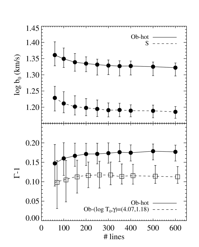
Figure 14: The intercept (upper panel) and slope (bottom panel) of the $b(N)$-cutoff for different numbers of absorption lines used in the fit. The cutoff depends weakly on the number of lines, although the statistical variance does increase significantly when the number of lines falls below 200. The numbers refer to the number of lines after removal of the lines with errors greater than 50%, but before applying the Hui-Rutledge cut. The error bars indicate 68% confidence intervals around the medians. The lower curve in the bottom panel has been slightly displaced.

While the statistical variance in the intercept of the $b(N)$-cutoff is small, the variance in the slope is comparable to the differences between models. Fortunately, we can do better than measuring the cutoff for the complete set of lines in an observed spectrum. The bootstrap method (drawing $n$ random lines from the complete set of $n$ lines, with replacement) can be used to generate a large number of synthetic data sets. These data sets can then be used to obtain approximations to the probability distributions for the parameters of the cutoff. Since bootstrap resampling replaces a random fraction of the original lines by duplicated original lines, a smaller fraction of the $b$-$N$ space around the cutoff is filled and the variance in the measured cutoff increases. Although the bootstrap distribution is generally broader than the true distribution, its median is a robust estimate of the true median. When dealing with observed spectra, we will use the medians of the bootstrap distributions as our best estimates of the parameters of the $b(N)$-cutoff. In section 6 we will use Monte Carlo simulations to estimate the variance in the bootstrap medians.

5 SYSTEMATIC EFFECTS

In section 3 we established the relation between the cutoff in the $b(N)$-distribution and the equation of state of the low-density gas. In this section we will investigate whether other processes can change this relation.

5.1 Cosmology

Cosmology affects not only the equation of state, but also determines the evolution of structure. Theuns et al. [Theuns et al. 1999a] showed that the $b$-parameter distribution depends on cosmology. In particular, they showed that the effect of peculiar velocity gradients on the line widths can be very different in different CDM variants. We have recomputed simulated spectra for model S after imposing the equation of state of the significantly hotter model Ob. In Fig. 15 the probability distributions of the parameters of the $b(N)$-cutoff are compared for model Ob (solid lines) and this new model, S-hot (dashed). The distributions are almost indistinguishable. Also plotted is model Ob-vel (dot-dashed), which was created by setting all peculiar velocities in model Ob to zero. Again, the probability distributions are almost unchanged.

Figure 15: Probability distributions for the intercept (left panel) and slope (right panel) of the $b(N)$-cutoff for models with identical equations of state, but different systematics. S-hot (dashed line) is model S with the equation of state of model Ob imposed. Ob-vel (dot-dashed) is identical to model Ob, but with all peculiar velocities set to zero. Ob+scat is model Ob with twice as much scatter around the equation of state. All distributions are determined using 500 sets of 300 random absorption lines, at $z=3$.

The line widths of many of the low column density lines are dominated by the Hubble flow. Fig. 16 illustrates the effect that changing the Hubble expansion has on the cutoff in the $b(N)$-distribution. The obvious way to change the Hubble flow is to change the Hubble constant. However, the equation of state also depends on the value of the Hubble constant. In order to isolate the effect of the Hubble flow, we changed the value of the Hubble constant in the analysis stage, i.e. just before computing the spectra, keeping the equation of state fixed. Increasing the value of the Hubble parameter at $z=3$ from a corresponding present day value of $h=0.65$ to 0.8 has no effect on the cutoff. Lowering $h$ to 0.5 shifts the slope to slightly larger values, but leaves the intercept unchanged.

Figure 16: Probability distributions for the intercept (left panel) and slope (right panel) of the $b(N)$-cutoff for models with identical equations of state, but different Hubble flow contributions to the line widths. For models Ob-h=50 and Ob-h=80 the spectra have been calculated using a Hubble parameter corresponding to a present day value of $h=0.5$ and $h=0.8$ respectively (Ob has $h=0.65$). All distributions are determined using 500 sets of 300 random absorption lines, at $z=3$.

We conclude that, unlike the $b$-distribution, the cutoff in the $b(N)$-distribution is independent of the assumed CDM model for a fixed equation of state.

5.2 Mean absorption

The optical depth in neutral hydrogen is proportional to the quantity $\Omega_{b}^{2}h^{3}/\Gamma_{\hbox{H\,{\sc i}}}$. Since it is still unclear what the dominant source of the metagalactic ionizing background is, the H i ionization rate, $\Gamma_{\hbox{H\,{\sc i}}}$, is uncertain. Changing $\Gamma_{\hbox{H\,{\sc i}}}$ has very little effect on the equation of state [Hui & Gnedin 1997], which means that the optical depth can be scaled to match the observed mean flux decrement in the analysis stage. However, the observations do show some scatter in the mean flux decrement. This scatter could be due to spatial variations of the ionizing background, or it could be caused by measurement errors. We therefore need to check whether errors in the assumed effective optical depth affect the relation between the cutoff and the equation of state.

Changing the effective optical depth by rescaling the ionizing background alters the relation between column density and gas density. This will shift the $b(N)$-distribution along the $N$-axis. Hence we expect the intercept of the cutoff to change and the slope to remain constant. In terms of our power-law model, increasing the photoionization rate (i.e. decreasing the effective optical depth) will increase the coefficient $A$ in equation 2 and thus increase the measured intercept $b_{0}$ for a given $T_{0}$ (equation 5), while leaving the slope $\Gamma-1$ constant (equation 6). Fig. 17 confirms these predictions. The dependence of $b_{0}$ on the effective optical depth turns out to be rather weak, even for models with a relatively steep cutoff. Realistic errors in the mean flux decrement (10–20% at $z\sim 3$) will give rise to errors in $b_{0}$ that are smaller than the statistical variance.

Figure 17: The intercept of the $b(N)$-cutoff decreases slightly with increasing absorption (upper panel). The slope of the cutoff and the effective optical depth appear to be uncorrelated (bottom panel). For realistic errors in the assumed effective optical depth (10–20% at $z\sim 3$), the error in the intercept is small compared to the statistical variance. Plotted data points are model Ob (filled circle) and models with rescaled background fluxes (open squares), all for 300 random lines at $z=3$. All models have the same equation of state. Error bars enclose 68% confidence intervals around the median values.

5.3 Signal to noise

The signal to noise ratio (S/N) per pixel in the simulated spectra is 50, comparable to the noise level in high-quality observations. However, spectra taken with for example the HIRES spectrograph on the KECK telescope have a S/N that varies across the spectrum. Fig. 18 illustrates the effect of changing the signal to noise (S/N) in the spectrum. The statistical variance in the cutoff increases rapidly when the S/N falls below 25. While the intercept increases slightly for S/N smaller than 25, the slope appears to be independent of the signal to noise. We therefore conclude that variations in the S/N in observed spectra are unimportant, as long as the signal to noise is greater than about 20.

Figure 18: The intercept (top panel) and slope (bottom panel) of the $b(N)$-cutoff as a function of signal to noise ratio (S/N). Variations in the S/N are unimportant as long as the S/N is greater than about 20. Plotted data points are all for 300 random lines taken from model Ob at $z=3$. All models have the same equation of state. Error bars enclose 68% confidence intervals around the median values.

5.4 Missing physics

Since the cosmological parameters and reionization history have yet to be fully constrained, the models used in this paper may not be correct. This will however not affect the results of this paper, as long as the bulk of the low-density gas follows a power-law equation of state. We should therefore ask if there are any physical processes, which have not been incorporated in the simulations, that could destroy the uniformity of the thermal state of the low-density gas. Feedback from massive stars and fluctuations in the spectrum of the photoionizing flux are two examples. Although these processes would predominantly affect the gas in virialized halos, they could introduce some additional scatter in the equation of state of the gas responsible for the low column density Ly$\alpha$ forest.

We recomputed simulated spectra for model Ob, after doubling the scatter around the fitted temperature-density relation. The $b(N)$-cutoff of this new model, Ob+scat, is indistinguishable from the one of model Ob (solid and dotted curves in Fig. 15). Note that although processes like feedback can heat the IGM locally, it is hard to think of any process, apart from adiabatic expansion, that could cool the low-density gas. Furthermore, whereas low-density gas that is heated to $T>T_{0}(\rho/\bar{\rho})^{\gamma-1}$ can only cool over a Hubble time, gas that is cooled below the equation of state is quickly reheated. Any additional scatter in the thermal state is thus unlikely to alter the cutoff in the gas temperature.

Any comparison between observations and simulations is complicated by the fact that observed spectra cover a much larger redshift path than the simulation boxes and therefore include effects like redshift evolution and cosmic variance, which are not present in the simulations. Large-scale fluctuations, especially in the ionization fraction (i.e. the relation between density and column density) could potentially distort the relation between the mean equation of state and the $b(N)$-cutoff.

Redshift evolution mainly affects the mean absorption and does so in a well defined manner, which can be modeled by comparing the observations to a combination of simulated spectra that have different effective optical depths. If the line of sight to the quasar passes an ionizing source, then lines from that region will be shifted to lower column densities and therefore have little effect on the measured $b(N)$-cutoff (since it increases with column density). Since the ionizing background originates from a collection of point sources, minima in the ionizing background would be shallower and more extended than maxima, except during reionization. In any case, if the sightline goes through a region where the mean neutral hydrogen density is substantially enhanced and therefore affects the measured cutoff, this will become clear when the spectrum is analyzed in redshift bins.

We conclude that even if local effects would produce a large scatter in the thermal state of the low-density gas, the relation between the mean equation of state and the $b(N)$-cutoff would remain unchanged.

6 MONTE CARLO SIMULATIONS

In section 4 we described how bootstrap resampling can be used to reduce the statistical variance in the measured $b(N)$-cutoff. Given a set of absorption lines from a single QSO spectrum, the bootstrap method is used to generate synthetic data sets, for which the cutoff is measured. The medians of the resulting probability distributions for the parameters of the cutoff are then used as best estimates of the true medians.

In order to see how well the equation of state can be measured, we performed Monte Carlo simulations. We drew 300 random lines, with column density in the range $10^{12.5}\,\rm cm^{-2}\leq N\leq 10^{14.5}\,\rm cm^{-2}$, from model Ob at $z=3$ and used the bootstrap method to generate probability distributions for the parameters of the cutoff. The median $\log b_{0}$ and $\Gamma$ were then converted to measurements of $\log T_{0}$ and $\gamma$ using the linear relations determined from the simulations. The statistical variance in the medians of the bootstrap distributions was estimated from 100 Monte Carlo simulations. For 300 lines per spectrum the dispersion in the median is: $\sigma_{\rm stat}(\log T_{0})=0.033$ (K), $\sigma_{\rm stat}(\gamma)=0.13$.

If multiple spectra are available, the statistical variance in the median can be reduced by summing the bootstrap probability distributions of the different spectra. Fig. 19 illustrates how the errors change when multiple spectra are used, each containing 100 (dashed curves) or 300 (solid curves) absorption lines in the column density range over which the cutoff is fitted. The bottom curve of each pair indicates the statistical $1\sigma$ error. The statistical dispersion asymptotes to the bin size used for determining the probability distributions.

Figure 19: The dispersion in the amplitude (top panel) and slope (bottom panel) of the equation of state as a function of the number of spectra used. The dispersion is computed from 100 Monte Carlo simulations of spectra with 100 (dashed curves) or 300 (solid curves) absorption lines each, at $z=3$. The lower curves indicate the statistical variance, while the upper curves give the total errors (statistical and systematic). Combining spectra has only limited effect since systematic errors dominate. The statistical errors asymptote to the bin size used for determining the probability distributions.

Besides the statistical variance in the median, there is some scatter around the linear relations between the parameters of the cutoff and the equation of state. For example, for 300 lines per spectrum at $z=3$, the systematic errors (i.e. the dispersion of the solid circles around the dashed lines in Figs. 9 and 10) in the parameters of the cutoff are $\sigma_{\rm sys}(\log b_{0})=0.009~{}({\rm km}\,{\rm s}^{-1})$ and $\sigma_{\rm sys}(\Gamma)=0.015$. The top curve of each pair in Fig. 19 indicates the total (statistical plus systematic) $1\sigma$ error.

For a single spectrum with 300 lines (typical for $z=3$), the predicted total errors are: $\sigma(\log T_{0})=0.040$ (K), $\sigma(\gamma)=0.17$. For three spectra the errors reduce to $\sigma(\log T_{0})=0.029$ (K) and $\sigma(\gamma)=0.13$. Adding more spectra has very little effect since systematic errors dominate. The errors are larger when there are only 100 absorption lines per spectrum. In this case the statistical variance is larger and the errors can be reduced significantly by adding more spectra. The fact that even for this small number of lines the constraints on the parameters of the equation of state are significant, suggests that the method will also work at $z\sim 2$.

7 SUMMARY AND DISCUSSION

Numerical simulations indicate that the smooth, photoionized intergalactic medium (IGM) responsible for the low column density Ly$\alpha$ forest follows a well defined temperature-density relation. For densities around the cosmic mean, shock-heating is negligible and the equation of state of the gas is well-described by a power-law $T=T_{0}(\rho/\bar{\rho})^{\gamma-1}$. The equation of state depends on cosmology, reionization history and the hard X-ray background. Although the absorption spectra can be fitted by a set of Voigt profiles, the lines do not in general correspond to discrete high-density gas clouds. Scatter plots of the distribution of line widths ($b$-parameters) as a function of column density ($N$) in observed QSO spectra clearly show a lower envelope, which increases with column density.

The decomposition of spectra produced by a fluctuating IGM into discrete Voigt profiles is artificial. However, the column density of the absorption lines correlates strongly with the density of the gas responsible for the absorption. Although the $b$-parameters are in general not correlated with the temperature of the gas, the line widths of the subset of lines that are close to the $b(N)$-cutoff do show a strong correlation with temperature. This implies that there exists a lower limit to the line width, set by the the thermal state of the absorbing gas, which in turn depends on its density. Hence the cutoff seen in the $b(N)$-distribution is a direct consequence of the existence of a temperature-density relation for the low-density gas and can be used to measure the equation of state of the IGM.

We developed an iterative procedure for fitting a power-law, $b=b_{0}(N/N_{0})^{\Gamma-1}$, to the $b(N)$-cutoff over a certain column density range ($10^{12.5}\,\rm cm^{-2}\leq N\leq 10^{14.5}\,\rm cm^{-2}$ at $z=3$). The algorithm is insensitive to unphysically narrow lines, which occur in blends and as unidentified metal lines. The intercept of the power-law, $\log b_{0}$, can be measured very precisely and is shown to be very sensitive to $\log T_{0}$ (Fig. 9). The slope of the cutoff, $\Gamma-1$, is proportional to $\gamma-1$, but the dependence is weak and it is harder to measure (Fig. 10).

The intercept of the $b(N)$-cutoff is a measure of the temperature of the gas responsible for the absorption lines that are used to determine the cutoff. This gas is typically slightly overdense and consequently the intercept depends on both $T_{0}$, the temperature at mean density, and $\gamma$, the slope of the equation of state. However, if we normalise the equation of state to the temperature at the characteristic density of the gas, $T=T_{\delta}(\rho/\rho_{\delta})^{\gamma-1}$, where $\rho_{\delta}\equiv\bar{\rho}(1+\delta)$, then the intercept of the cutoff depends only on the amplitude of the equation of state, $T_{\delta}$.

The relation between the cutoff and the equation of state is independent of the assumed cosmology (for a fixed equation of state). In particular, it remains unchanged when all peculiar velocities are set to zero and when the contribution of the Hubble flow to the line widths is varied. Changing the effective optical depth (i.e. rescaling the ionizing background), alters the relation between column density and gas density and thus the relation between $\log b_{0}$ and $\log T_{0}$. However, the dependence is weak and realistic errors in the measured mean absorption do not lead to significant errors in the derived value of $T_{0}$. Variations in the signal to noise ratio are also unimportant, as long as the ratio is greater than about 20.

The simulations used to determine the relation between the cutoff and the equation of state do not incorporate some potentially important physical processes, like feedback from e.g. star formation. This will however not change the results presented in this paper, as long as the bulk of the low-density gas follows a power-law equation of state. Since local effects like feedback would increase the temperature and since gas cooled to a temperature below that given by the equation of state is quickly reheated, any additional scatter in the thermal state of the gas is unlikely to affect the cutoff in the gas temperature. Doubling the scatter around the equation of state has no discernible effect on the $b(N)$-cutoff.

The finite number of absorption lines per QSO spectrum introduces statistical variance in the measured cutoff. The statistical variance can be reduced by using the bootstrap method to generate probability distributions for the parameters of the cutoff and using the medians as the best estimates of the true parameters. If multiple spectra are available, the variance can be further reduced by adding the bootstrap distributions of the different spectra. We use Monte Carlo simulations to estimate the statistical variance in the medians of the bootstrap distributions. Besides the statistical variance, there is a systematic uncertainty from the scatter in the linear relations between the parameters of the cutoff and the equation of state.

For a single spectrum at $z=3$ we predict the following total (statistical plus systematic) errors: $\sigma(\log T_{0})=0.040$ (K) ($\Delta T_{0}/T_{0}=0.09$), $\sigma(\gamma)=0.17$. For three spectra the errors reduce to $\sigma(\log T_{0})=0.029$ (K) ($\Delta T_{0}/T_{0}=0.07$) and $\sigma(\gamma)=0.13$. Increasing the number of spectra beyond three has very little effect on the total uncertainty because systematic errors dominate. These errors should be compared to the ranges considered to be physically reasonable, $10^{3.0}\,\rm K<T_{0}<10^{4.5}\,\rm K$ and $1.2<\gamma<1.7$ [Hui, Gnedin & Zhang 1997, Hui & Gnedin 1997].

The analysis presented in this paper is for redshift $z=3$. At smaller redshifts, the constraints will be less tight because of the smaller number of lines per spectrum. However, we showed that even for one third of the number of lines typical at $z=3$, the constraints on the equation of state are significant. Furthermore, the statistical variance can be reduced by using multiple spectra. At higher redshifts the errors will also be somewhat larger than at $z=3$, mainly because the higher density of lines increases the number of blends and the errors in the continuum fit.

When using the simulations to convert the observed $b(N)$-cutoff into an equation of state, one has to be careful to treat the observed and simulated spectra in the same way. For example, the simulated and observed $b(N)$-distributions should have the same number of lines and the same continuum and Voigt profile fitting algorithms should be used for the simulated and observed spectra.

Given the existence of many high quality quasar absorption line spectra, it should be possible to greatly reduce the uncertainty in the equation of state of the low-density gas over the range $z=2-4$. This will allow us to put significant constraints on the reionization history of the universe.

References

- [Abel & Haehnelt 1999] Abel T., Haehnelt M.G., 1999, preprint (astro-ph/9903102)
- [Bryan et al. 1998] Bryan G.L., Machacek M., Anninos P., Norman M.L., 1998, ApJ, in press (astro-ph/9805340)
- [Carswell et al. 1987] Carswell R.F., Webb J.K., Baldwin J.A., Atwood B., 1987, ApJ, 319, 709
- [e.g. Cen et al. 1994] Cen R., Miralda-Escudé J., Ostriker J.P., Rauch M., 1994, ApJL, 437, L83
- [Couchman, Thomas & Pearce 1995] Couchman H.M.P., Thomas P.A., Pearce F.P., 1995, ApJ, 452, 797
- [Davé et al. 1999] Davé R., Hernquist L., Katz N., Weinberg D.H., 1999, ApJ, 511, 521
- [Eke, Cole & Frenk 1996] Eke V.R., Cole S., Frenk C.S., 1996, MNRAS, 282, 263
- [Gingold & Monaghan 1977] Gingold R.A., Monaghan J.J., 1977, MNRAS, 181, 375
- [Gunn & Peterson 1965] Gunn J.E., Peterson B.A., 1965, ApJ, 142, 1633
- [Haardt & Madau 1996] Haardt F., Madau P., 1996, ApJ, 461, 20
- [Haehnelt & Steinmetz 1998] Haehnelt M.G., Steinmetz M., 1998, MNRAS, 298, L21
- [Hernquist et al. 1996] Hernquist L., Katz N., Weinberg D.H., Miralda-Escudé J., 1996, ApJL, 457, L51
- [e.g. Hu et al. 1995] Hu E.M., Kim T., Cowie L.L., Songaila A., Rauch M., 1995, AJ, 110, 1526
- [Hui & Gnedin 1997] Hui L., Gnedin N., 1997, MNRAS, 292, 27
- [Hui, Gnedin & Zhang 1997] Hui L., Gnedin N., Zhang, Y., 1997, MNRAS, 486, 599
- [Hui & Rutledge 1997] Hui L., Rutledge R., 1997, preprint (astro-ph/9709100)
- [Kim et al. 1997] Kim T., Hu E.M., Cowie L.L., Songaila A., 1997, AJ, 114, 1
- [Kirkman & Tytler 1997] Kirkman D., Tytler, D., 1997, ApJ, 484, 672
- [Lu et al. 1996] Lu L., Sargent W.L.W., Womble D.S., Takada-Hidai M., 1996, ApJ, 472, 509
- [Lucy 1970] Lucy L.B., 1977, AJ, 82, 1023
- [Madau & Efstathiou 1999] Madau P., Efstathiou G., ApJ, in press (astro-ph/9902080)
- [Miralda-Escudé et al. 1996] Miralda-Escudé J., Cen R., Ostriker J.P., Rauch M., 1996, ApJ, 471, 582
- [Nath, Sethi & Shchekinov 1999] Nath B.B., Sethi S.K., Shchekinov Y., 1999, MNRAS, 303, 1
- [Pettini et al. 1990] Pettini M., Hunstead R.W., Smith L.J., Mar D.P., 1990, MNRAS, 246, 545
- [Rauch et al. 1993] Rauch M., Carswell R.F., Webb J.K., Weymann R.J., 1993, MNRAS, 260, 589
- [Rauch et al. 1997] Rauch M., Miralda-Escudé J., Sargent W.L.W., Barlow T.A., Weinberg D.H., Hernquist L., Katz N., Cen R., Ostriker J.P., 1997, ApJ, 489, 7
- [Rauch 1998] Rauch M., 1998, ARA&A, 36, 267
- [Theuns, Leonard & Efstathiou 1998] Theuns T., Leonard A., Efstathiou G., 1998, MNRAS, 297, L49
- [Theuns et al. 1998] Theuns T., Leonard A., Efstathiou G., Pearce F.R., Thomas P.A., 1998, MNRAS, 301, 478
- [Theuns et al. 1999a] Theuns T., Leonard A., Schaye J., Efstathiou G., 1999a, MNRAS, 303, L58
- [Theuns et al. 1999b] Theuns T., Schaye J., Haehnelt M., 1999b, MNRAS, in preparation
- [Zhang, Anninos & Norman 1995] Zhang Y., Anninos P., Norman M.L., 1995, ApJL, 453, L57
- [Zhang et al. 1997] Zhang Y., Anninos P., Norman M.L., Meiksin A., 1997, ApJ, 485, 496