Spectral Analysis of Stellar Light Curves by Means of Neural Networks

Abstract

Periodicity analysis of unevenly collected data is a relevant issue in several scientific fields. In astrophysics, for example, we have to find the fundamental period of light or radial velocity curves which are unevenly sampled observations of stars. Classical spectral analysis methods are unsatisfactory to solve the problem. In this paper we present a neural network based estimator system which performs well the frequency extraction in unevenly sampled signals. It uses an unsupervised Hebbian nonlinear neural algorithm to extract, from the interpolated signal, the principal components which, in turn, are used by the MUSIC frequency estimator algorithm to extract the frequencies. The neural network is tolerant to noise and works well also with few points in the sequence. We benchmark the system on synthetic and real signals with the Periodogram and with the Cramer-Rao lower bound.

1 Introduction

The search for periodicities in time or spatial dependent signals is a topic of the uttermost relevance in many fields of research, from geology (stratigraphy, seismology, etc.; (Brescia et al. 1996) ) to astronomy (Barone et al. 1994) where it finds wide application in the study of light curves of variable stars, AGN’s, etc.

The more sensitive instrumentation and observational techniques become, the more frequently we find variable signals in time domain that previously were believed to be constant. Research for possible periodicities in the signal curves is then a natural consequence, when not an important issue. One of the most relevant problems concerning the techniques of periodic signal analysis is the way in which data are collected: many time series are collected at unevenly sampling rate. We have two types of problems related either to unknown fundamental period of the data, or their unknown multiple periodicities. Typical cases, for instance in Astronomy, are the determination of the fundamental period of eclipsing binaries both of light and radial velocity curves, or the multiple periodicities determination of ligth curves of pulsating stars. The difficulty arising from unevenly spaced data is rather obvious and many attempts have been made to solve the problem in a more or less satisfactory way. In this paper we will propose a new way to approach the problem using neural networks, that seems to work satisfactory well and seems to overcome most of the problems encountered when dealing with unevenly sampled data.

2 Spectral analysis and unevenly spaced data

2.1 Introduction

In what follows, we assume $x$ to be a physical variable measured at discrete times $t_{i}$. ${x(t_{i})}$ can be written as the sum of the signal $x_{s}$ and random errors $R$: $x_{i}=x(t_{i})=x_{s}(t_{i})+R(t_{i})$. The problem we are dealing with is how to estimate fundamental frequencies which may be present in the signal $x_{s}(t_{i})$ (Deeming 1975; Kay 1988; Marple 1987).

If $x$ is measured at uniform time steps (even sampling) (Horne & Baliunas 1986; Scargle 1982) there are a lot of tools to effectively solve the problem which are based on Fourier analysis (Kay 1988; Marple 1987; Oppennheim & Schafer 1965). These methods, however, are usually unreliable for unevenly sampled data. For instance, the typical approach of resampling the data into an evenly sampled sequence, through interpolation, introduces a strong amplification of the noise which affects the effectiveness of all Fourier based techniques which are strongly dependent on the noise level (Horowitz 1974).

There are other techniques used in specific areas (Ferraz-Mello 1981; Lomb 1976): however, none of them faces directly the problem, so that they are not truly reliable. The most used tool for periodicity analysis of evenly or unevenly sampled signals is the Periodogram (Lomb 1976; Scargle 1982); therefore we will refer to it to evaluate our system.

2.2 Periodogram and its variations

The Periodogram (P), is an estimator of the signal energy in the frequency domain (Deeming 1975; Kay 1988; Marple 1987; Oppennheim & Schafer 1965). It has been extensively applied to pulsating star light curves, unevenly spaced, but there are difficulties in its use, specially concerning with aliasing effects.

2.2.1 Scargle’s Periodogram

This tool is a variation of the classical P. It was introduced by J.D. Scargle (Scargle 1982) for these reasons: 1) data from instrumental sampling are often not equally spaced; 2) due to P inconsistency (Kay 1988; Marple 1987; Oppennheim & Schafer 1965), we must introduce a selection criterion for signal components.

In fact, in the case of even sampling, the classical P has a simple statistic distribution: it is exponentially distributed for Gaussian noise. In the uneven sampling case the distribution becomes very complex. However, Scargle’s P has the same distribution of the even case (Scargle 1982). Its definition is:

$$P_{x}(f) = \frac{1}{2}\frac{[\sum_{n=0}^{N-1}x(n)\cos 2\pi f(t_{n}-\tau)]^{2}}{\sum_{n=0}^{N-1}\cos^{2}2\pi f(t_{n}-\tau)}+$$ (1)

$$\frac{[\sum_{n=0}^{N-1}x(n)\sin 2\pi f(t_{n}-\tau)]^{2}}{\sum_{n=0}^{N-1}\sin^{2}2\pi f(t_{n}-\tau)}$$

where

$$\tau=\frac{1}{4\pi f}\frac{\sum_{n=0}^{N-1}\sin 4\pi ft_{n}}{\sum_{n=0}^{N-1}\cos 4\pi ft_{n}}$$

and $\tau$ is a shift variable on the time axis, $f$ is the frequency, $\{x\left(n\right),t_{n}\}$ is the observation series.

2.2.2 Lomb’s Periodogram

This tool is another variation of the classical P and is similar to the Scargle’s P. It was introduced by Lomb (Lomb 1976) and we used the Numerical Recipes in C release (Numerical Recipes in C 1988-1992).

Let us suppose to have $N$ points $x(n)$ and to compute mean and variance:

$$\bar{x}=\frac{1}{N}\sum_{n=1}^{N}x(n)\qquad\qquad\sigma^{2}=\frac{1}{N-1}\sum_{n=1}^{N}\left(x(n)-\bar{x}\right)^{2}.$$ (2)

Therefore, the normalised Lomb’s P (power spectra as function of an angular frequency $\omega\equiv 2\pi f>0$) is defined as follows

$$P_{N}(\omega) = \frac{1}{2\sigma^{2}}\left[\frac{[\sum_{n=0}^{N-1}\left(x(n)-\bar{x}\right)\cos\omega(t_{n}-\tau)]^{2}}{\sum_{n=0}^{N-1}\cos^{2}\omega(t_{n}-\tau)}\right]+$$ (3)

$$+\frac{1}{2\sigma^{2}}\left[\frac{[\sum_{n=0}^{N-1}\left(x(n)-\bar{x}\right)\sin\omega(t_{n}-\tau)]^{2}}{\sum_{n=0}^{N-1}\sin^{2}\omega(t_{n}-\tau)}\right]$$

where $\tau$ is defined by the equation

$$\tan\left(2\omega\tau\right)=\frac{\sum_{n=0}^{N-1}\sin 2\omega t_{n}}{\sum_{n=0}^{N-1}\cos 2\omega t_{n}}$$

and $\tau$ is an offset, $\omega$ is the frequency, $\{x\left(n\right),t_{n}\}$ is the observation series. The horizontal lines in the figures 19, 22, 25, 27, 32 and 34 correspond to the practical significance levels, as indicated in (Numerical Recipes in C 1988-1992).

2.3 Modern spectral analysis

Frequency estimation of narrow band signals in Gaussian noise is a problem related to many fields (Kay 1988; Marple 1987). Since the classical methods of Fourier analysis suffer from statistic and resolution problems, then newer techniques based on the analysis of the signal autocorrelation matrix eigenvectors were introduced (Kay 1988; Marple 1987).

2.3.1 Spectral analysis with eigenvectors

Let us assume to have a signal with p sinusoidal components (narrow band). The p sinusoids are modelled as a stationary ergodic signal, and this is possible only if the phases are assumed to be indipendent random variables uniformly distributed in $[0,2\pi)$ (Kay 1988; Marple 1987). To estimate the frequencies we exploit the properties of the signal autocorrelation matrix (a.m.) (Kay 1988; Marple 1987). The a.m. is the sum of the signal and the noise matrices; the p principal eigenvectors of the signal matrix allow the estimate of frequencies; the p principal eigenvectors of the signal matrix are the same of the total matrix.

3 PCA Neural Nets

3.1 Introduction

Principal Component analysis (PCA) is a widely used technique in data analysis. Mathematically, it is defined as follows: let ${\bf C}=E({\bf x}{\bf x}^{T})$ be the covariance matrix of L-dimensional zero mean input data vectors ${\bf x}$. The i-th principal component of ${\bf x}$ is defined as ${\bf x}^{T}{\bf c}(i)$, where ${\bf c}(i)$ is the normalized eigenvector of C corresponding to the i-th largest eigenvalue $\lambda(i)$. The subspace spanned by the principal eigenvectors ${\bf c}(1),\ldots,{\bf c}(M),(M<L))$ is called the PCA subspace (of dimensionality M) (Oja et al. 1991; Oja et al. 1996). PCA’s can be neurally realized in various ways (Baldi & Hornik 1989; Jutten & Herault 1991; Oja 1982; Oja et al. 1991; Plumbley 1993; Sanger 1989). The PCA neural network used by us is a one layer feedforward neural network which is able to extract the principal components of the stream of input vectors. Typically, Hebbian type learning rules are used, based on the one unit learning algorithm originally proposed by Oja (Oja 1982). Many different versions and extensions of this basic algorithm have been proposed during the recent years; see (Karhunen & Joutsensalo 1994; Karhunen & Joutsensalo 1995; Oja et al. 1996; Sanger 1989).

3.2 Linear, robust, nonlinear PCA Neural Nets

The structure of the PCA neural network can be summarised as follows (Karhunen & Joutsensalo 1994; Karhunen & Joutsensalo 1995; Oja et al. 1996; Sanger 1989): there is one input layer, and one forward layer of neurons totally connected to the inputs; during the learning phase there are feedback links among neurons, that classify the network structure as either hierarchical or symmetric. After the learning phase the network becomes purely feedforward. The hierarchical case leads to the well known GHA algorithm (Karhunen & Joutsensalo 1995; Sanger 1989); in the symmetric case we have the Oja’s subspace network (Oja 1982).

PCA neural algorithms can be derived from optimisation problems, such as variance maximization and representation error minimisation (Karhunen & Joutsensalo 1994; Karhunen & Joutsensalo 1995) so obtaining nonlinear algorithms (and relative neural networks). These neural networks have the same architecture of the linear ones: either hierarchical or symmetric. These learning algorithms can be further classified in: robust PCA algorithms and nonlinear PCA algorithms. We define robust a PCA algorithm When the objective function grows less than quadratically (Karhunen & Joutsensalo 1994; Karhunen & Joutsensalo 1995). The nonlinear learning function appears at selected places only. In nonlinear PCA algorithms all the outputs of the neurons are nonlinear function of the responses.

3.2.1 Robust PCA algorithms

In the robust generalization of variance maximisation, the objective function $f(t)$ is assumed to be a valid cost function (Karhunen & Joutsensalo 1994; Karhunen & Joutsensalo 1995), such as $\ln\cos(t)$ e $|t|$. This leads to the algorithm:

$${\bf w}_{k+1}(i) = {\bf w}_{k}(i)+\mu_{k}g(y_{k}(i)){\bf e}_{k}(i),$$ (4)

$$\qquad{\bf e}_{k}(i) = {\bf x}_{k}-\sum_{j=1}^{I(i)}y_{k}(j){\bf w}_{k}(j)$$

In the hierarchical case we have $I(i)=i$. In the symmetric case $I(i)=M$, the error vector ${\bf e}_{k}(i)$ becomes the same ${\bf e}_{k}$ for all the neurons, and equation(4) can be compactly written as:

$${\bf W}_{k+1}={\bf W}_{k}+\mu{\bf e}_{k}g({\bf y}_{k}^{T})$$ (5)

where ${\bf y}={\bf W}^{T}_{k}{\bf x}$ is the instantaneous vector of neuron responses. The learning function $g$, derivative of $f$, is applied separately to each component of the argument vector.

The robust generalisation of the representation error problem (Karhunen & Joutsensalo 1994; Karhunen & Joutsensalo 1995), with $f(t)\leq t^{2}$, leads to the stochastic gradient algorithm :

$${\bf w}_{k+1}(i) = {\bf w}_{k}(i)+\mu({\bf w}_{k}(i)^{T}g({\bf e}_{k}(i)){\bf x}_{k}+$$

$$+ {\bf x}_{k}^{T}{\bf w}_{k}(i)g({\bf e}_{k}(i)))$$

This algorithm can be again considered in both hierarchical and symmetric cases. In the symmetric case $I(i)=M$, the error vector is the same $({\bf e}_{k})$ for all the weights ${\bf w}_{k}$. In the hierarchical case $I(i)=i$, equation(3.2.1) gives the robust counterparts of principal eigenvectors ${\bf c}(i)$.

3.2.2 Approximated Algorithms

The first update term ${\bf w}_{k}(i)^{T}g({\bf e}_{k}(i)){\bf x}_{k}$ in eq.(3.2.1) is proportional to the same vector ${\bf x}_{k}$ for all weights ${\bf w}_{k}(i)$. Furthermore, we can assume that the error vector ${\bf e}_{k}$ should be relatively small after the initial convergence. Hence, we can neglet the first term in equation(3.2.1) and this leads to:

$${\bf w}_{k+1}(i)={\bf w}_{k}(i)+\mu{\bf x}_{k}^{T}y_{k}(i)g({\bf e}_{k}(i))$$ (7)

3.2.3 Nonlinear PCA Algorithms

Let us consider now the nonlinear extensions of PCA algorithms. We can obtain them in a heuristic way by requiring all neuron outputs to be always nonlinear in the equation(4) (Karhunen & Joutsensalo 1994; Karhunen & Joutsensalo 1995). This leads to:

$${\bf w}_{k+1}(i) = {\bf w}_{k}(i)+\mu g(y_{k}(i)){\bf b}_{k}(i),$$ (8)

$$\qquad{\bf b}_{k}(i) = {\bf x}_{k}-\sum_{j=1}^{I(i)}g(y_{k}(j)){\bf w}_{k}(j)\quad\forall i=1,\ldots,p$$

4 Independent Component Analysis

Independent Component Analysis (ICA) is a useful extension of PCA that was developed in context with source or signal separation applications (Oja et al. 1996): instead of requiring that the coefficients of a linear expansion of data vectors are uncorrelated, in ICA they must be mutually independent or as independent as possible. This implies that second order moments are not sufficient, but higher order statistics are needed in determining ICA. This provides a more meaningful representation of data than PCA. In current ICA methods based on PCA neural networks, the following data model is usually assumed. The $L$-dimensional $k$-th data vector ${\bf x}_{k}$ is of the form (Oja et al. 1996):

$${\bf x}_{k}={\bf As}_{k}+{\bf n}_{k}=\sum_{i=1}^{M}s_{k}(i){\bf a}(i)+{\bf n}_{k}$$ (9)

where in the M-vector ${\bf s}_{k}=[s_{k}(1),\ldots,s_{k}(M)]^{T}$, $s_{k}(i)$ denotes the $i$-th independent component (source signal) at time $k$, ${\bf A}=[{\bf a}(1),\ldots,{\bf a}(M)]$ is a $L\times M$ mixing matrix whose columns ${\bf a}(i)$ are the basis vectors of ICA, and ${\bf n}_{k}$ denotes noise.

The source separation problem is now to find an $M\times L$ separating matrix ${\bf B}$ so that the $M$-vector ${\bf y}_{k}={\bf Bx}_{k}$ is an estimate ${\bf y}_{k}={\bf\hat{s}}_{k}$ of the original independent source signal (Oja et al. 1996).

4.1 Whitening

Whitening is a linear transformation ${\bf A}$ such that, given a matrix ${\bf C}$, we have ${\bf ACA}^{T}={\bf D}$ where ${\bf D}$ is a diagonal matrix with positive elements (Kay 1988; Marple 1987).

Several separation algorithms utilise the fact that if the data vectors ${\bf x}_{k}$ are first pre-processed by whitening them (i.e. $E(x_{k}x_{k}^{T})=I$ with $E(.)$ denoting the expectation), then the separating matrix ${\bf B}$ becomes orthogonal (${\bf BB^{T}=I}$ see (Oja et al. 1996)).

Approximating contrast functions which are maximised for a separating matrix have been introduced because the involved probability densities are unknown (Oja et al. 1996).

It can be shown that, for prewhitened input vectors, the simpler contrast function given by the sum of kurtoses is maximised by a separating matrix ${\bf B}$ (Oja et al. 1996).

However, we found that in our experiments the whitening was not as good as we expected, because the estimated frequencies calculated for prewhitened signals with the neural estimator (n.e.) were not too much accurate.

In fact we can pre-elaborate the signal, whitening it, and then we can apply the n.e. . Otherwise we can apply the whitening and separate the signal in independent components with the nonlinear neural algorithm of equation(8) and then apply the n.e. to each of these components and estimate the single frequencies separately.

The first method gives comparable or worse results than n.e. without whitening. The second one gives worse results and is very expensive. When we used the whitening in our n.e. the results were worse and more time consuming than the ones obtained using the standard n.e. (i.e. without whitening the signal). Experimental results are given in the following sections. For these reasons whitening is not a suitable technique to improve our n.e. .

5 The neural network based estimator system

The process for periodicity analysis can be divided in the following steps:

- Preprocessing

We first interpolate the data with a simple linear fitting and then calculate and subtract the average pattern to obtain zero mean process (Karhunen & Joutsensalo 1994; Karhunen & Joutsensalo 1995).

- Neural computing

The fundamental learning parameters are:

1) the initial weight matrix;

2) the number of neurons, that is the number of principal eigenvectors that we need, equal to twice the number of signal periodicities (for real signals);

3) $\epsilon$, i.e. the threshold parameter for convergence ;

4) $\alpha$, the nonlinear learning function parameter;

5) $\mu$, that is the learning rate.

We initialise the weight matrix ${\bf W}$ assigning the classical small random values. Otherwise we can use the first patterns of the signal as the columns of the matrix: experimental results show that the latter technique speeds up the convergence of our neural estimator (n.e.). However, it cannot be used with anomalously shaped signals, such as stratigraphic geological signals.

Experimental results show that $\alpha$ can be fixed to : $1.$, $5.$, $10.$, $20.$, even if for symmetric networks a smaller value of $\alpha$ is preferable for convergence reasons. Moreover, the learning rate $\mu$ can be decreased during the learning phase, but we fixed it between $0.05$ and $0.0001$ in our experiments.

We use a simple criterion to decide if the neural network has reached the convergence: we calculate the distance between the weight matrix at step $k+1$, ${\bf W}_{k+1}$, and the matrix at the previous step ${\bf W}_{k}$, and if this distance is less than a fixed error threshold ($\epsilon$) we stop the learning process.

We finally have the following general algorithm in which STEP 4 is one of the neural learning algorithms seen above in section 3:

• STEP 1 Initialise the weight vectors ${\bf w}_{0}(i)\quad\forall i=1,\ldots,p$ with small random values, or with orthonormalised signal patterns. Initialise the learning threshold $\epsilon$, the learning rate $\mu$. Reset pattern counter $k=0$.

• STEP 2 Input the k-th pattern ${\bf x}_{k}=[x(k),\ldots,x(k+N+1)]$ where $N$ is the number of input components.

• STEP 3 Calculate the output for each neuron $y(j)={\bf w}^{T}(j){\bf x}_{i}\qquad\forall i=1,\ldots,p$.

• STEP 4 Modify the weights ${\bf w}_{k+1}(i)={\bf w}_{k}(i)+\mu_{k}g(y_{k}(i)){\bf e}_{k}(i)\qquad\forall i=1,\ldots,p$.

• STEP 5 Calculate

  $$testnorma=\sqrt{\sum_{j=1}^{p}\sum_{i=1}^{N}({\bf w}_{k+1}(ij)-{\bf w}_{k}(ij))^{2}}.$$ (10)

• STEP 6 Convergence test: if $(testnorma<\epsilon)$ then goto STEP 8.

• STEP 7 $k=k+1$. Goto STEP 2.

• STEP 8 End.

- Frequency estimator

We exploit the frequency estimator Multiple Signal Classificator (MUSIC). It takes as input the weight matrix columns after the learning. The estimated signal frequencies are obtained as the peak locations of the following function (Kay 1988; Marple 1987):

$$P_{MUSIC}=\log(\frac{1}{1-\sum_{i=1}^{M}|{\bf e}_{f}^{H}{\bf w}(i)|^{2}})$$ (11)

where ${\bf w}(i)$ is the $i-$th weight vector after learning, and ${\bf e}_{f}^{H}$ is the pure sinusoidal vector : ${\bf e}_{f}^{H}=[1,e_{f}^{j2\pi f},\ldots,e_{f}^{j2\pi f(L-1)}]^{H}$.

When $f$ is the frequency of the $i-$th sinusoidal component, $f=f_{i}$, we have ${\bf e}={\bf e}_{i}$ and $P_{MUSIC}\to\infty$. In practice we have a peak near and in correspondence of the component frequency. Estimates are related to the highest peaks.

6 Music and the Cramer-Rao Lower Bound

In this section we show the relation between the Music estimator and the Cramer-Rao bound following the notation and the conditions proposed by Stoica and Nehorai in their paper (Stoica and Nehorai 1990).

6.1 The model

The problem under consideration is to determine the parameters of the following model:

$${\bf y}(t)=A({\bf\theta}){\bf x}(t)+{\bf e}(t)$$ (12)

where $\left\{{\bf y}(t)\right\}\in C^{m\times 1}$ are the vectors of the observed data, $\left\{{\bf x}(t)\right\}\in C^{n\times 1}$ are the unknown vectors and ${\bf e}(t)\in C^{m\times 1}$ is the added noise; the matrix $A(\theta)\in C^{m\times n}$ and the vector $\theta$ are given by

$$A({\bf\theta})=\left[{\bf a}\left(\omega_{1}\right)...{\bf a}\left(\omega_{n}\right)\right];\qquad\qquad{\bf\theta}=\left[\omega_{1}...\omega_{n}\right]$$ (13)

where ${\bf a}\left(\omega\right)$ varies with the applications. Our aim is to estimate the unknown parameters of ${\bf\theta}$. The dimension $n$ of ${\bf x}(t)$ is supposed to be known a priori and the estimate of the parameters of ${\bf x}(t)$ is easy once ${\bf\theta}$ is known.

Now, we reformulate MUSIC to follow the above notation. The MUSIC estimate is given by the position of the $n$ smallest values of the following function:

$$f\left(\omega\right)={\bf a}^{\ast}\left(\omega\right)\hat{G}\hat{G}^{\ast}{\bf a}\left(\omega\right)={\bf a}^{\ast}\left(\omega\right)\left[I-\hat{S}\hat{S}^{\ast}\right]{\bf a}\left(\omega\right)$$ (14)

From equation(14) we can define the estimation error of a given parameter. $\left\{\hat{\omega}_{i}-\omega_{i}\right\}$ has (for big $N$) an asintotic gaussian distribution, with $0$ mean and with the following covariance matrix:

$$C_{MU}=\frac{\sigma}{2n}\left(H\circ I\right)^{-1}Re\left\{H\circ\left(A^{\ast}UA\right)^{T}\right\}\left(H\circ I\right)^{-1}$$ (15)

where $Re\left(x\right)$ is the real part of $x$, where

$$H=D^{\ast}GG^{\ast}D=D^{\ast}\left[I-A\left(A^{\ast}A\right)^{-1}A^{\ast}\right]D$$ (16)

and where $U$ is implicitly defined by:

$$A^{\ast}UA=P^{-1}+\sigma P^{-1}\left(A^{\ast}A\right)^{-1}P^{-1}$$ (17)

where $P$ is the covariance matrix of $x\left(t\right)$. The elements of the diagonal of the matrix $C_{MU}$ are the variances of the estimation error. On the other hand, the Cramer-Rao lower bound of the covariance matrix of every estimator of ${\bf\theta}$, for large $N$, is given by:

$$C_{CR}=\frac{\sigma}{2n}\left\{Re\left[H\circ P^{T}\right]\right\}^{-1}.$$ (18)

Therefore the statistical efficiency can be defined with the condition that P is diagonal as:

$$\left[C_{MU}\right]_{ii}\geq\left[C_{CR}\right]_{ii}$$ (19)

where the equality is reached when $m$ increases if and only if

$${\bf a}^{\ast}\left(\omega\right){\bf a}\left(\omega\right)\longrightarrow\infty\qquad\qquad as\quad m\longrightarrow\infty.$$ (20)

For $P$ non-diagonal, $\left[C_{MU}\right]_{ii}>\left[C_{CR}\right]_{ii}$. To adapt the model used in the spectral analysis

$${\bf y}(k)=\sum_{i=1}^{p}A_{i}e^{j\omega_{i}k}+{\bf e}(k)\qquad\qquad k=1,2,...,M$$ (21)

where $M$ is the total number of samples, to equation(14) we make the following transformations, after fixing an integer $m>p$:

$${\bf y}(t) = \left[y_{t}\quad...\quad y_{t+m-1}\right]$$

$${\bf a}\left(\omega\right) = \left[1\quad e^{j\omega}\quad e^{j\omega\left(m-1\right)}\right]$$ (22)

$${\bf x}(t) = \left[A_{1}e^{j\omega_{1}t}\quad...\quad A_{n}e^{j\omega_{n}t}\right]\qquad t=1,...,M-m+1$$

In this way our model satisfies the conditions of (Stoica and Nehorai 1990). Moreover, equations(22) depend on the choice of $m$ which influences the minimum error variance.

6.2 Comparison between PCA-MUSIC and the Cramer-Rao lower bound

In this subsection we compare the n.e. method with the Cramer-Rao lower bound, by varying the frequencies distance, the parameters $M$ and $m$ and the noise variance.

From the experiments it derives that, fixed $M$ and $m$, by varying the noise (white Gaussian) variance, the n.e. estimate is more accurate for small values of the noise variance as shown in figures 1-3. For $\Delta\omega$ small, the noise variance is far from the bound. By increasing $m$ the estimate improves, but there is a sensitivity to the noise (figures 4-6). By varying $M$, there is a sensitivity of the estimator to the number of points and to $m$ (figures 7-8). In fact, if we have a quite large number of points we reach the bound as illustrated in figures 9-10.

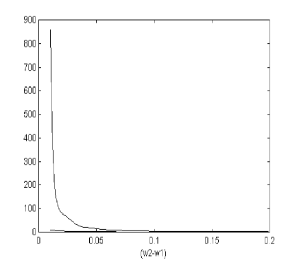
Figure 1: CRB and standard deviation of n.e. estimates; abscissa is the distance between the frequencies $\omega_{2}$ and $\omega_{1}$.
CRB (down); standard deviation of n.e. (up) with $m=5$, $\sigma=0.5$ and $M=50$.

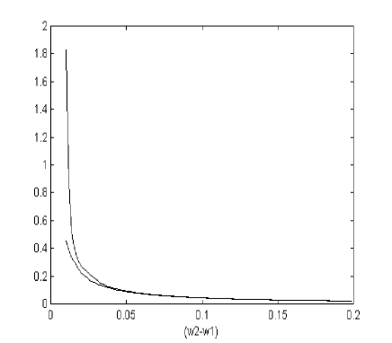
Figure 2: CRB and standard deviation of n.e. estimates; abscissa is the distance between the frequencies $\omega_{2}$ and $\omega_{1}$.
CRB (down); standard deviation of n.e. (up) with $m=5$, $\sigma=0.001$ and $M=50$.

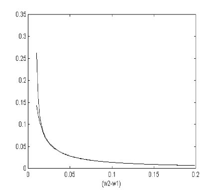
Figure 3: CRB and standard deviation of n.e. estimates; abscissa is the distance between the frequencies $\omega_{2}$ and $\omega_{1}$.
CRB (down); standard deviation of n.e. (up) with $m=5$, $\sigma=0.0001$ and $M=50$.

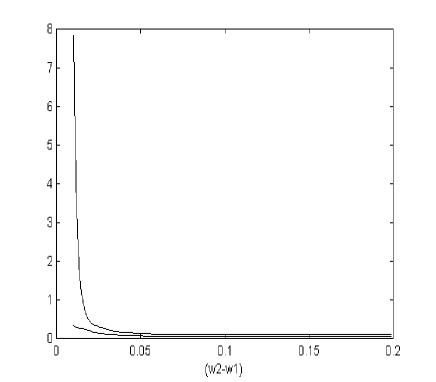
Figure 4: CRB and standard deviation of n.e. estimates; abscissa is the distance between the frequencies $\omega_{2}$ and $\omega_{1}$.
CRB (down); standard deviation of n.e. (up) with $m=20$, $\sigma=0.5$ and $M=50$.

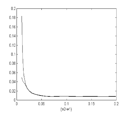
Figure 5: CRB and standard deviation of n.e. estimates; abscissa is the distance between the frequencies $\omega_{2}$ and $\omega_{1}$.
CRB (down); standard deviation of n.e. (up) with $m=20$, $\sigma=0.01$ and $M=50$.

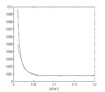
Figure 6: CRB and standard deviation of n.e. estimates; abscissa is the distance between the frequencies $\omega_{2}$ and $\omega_{1}$.
CRB (down); standard deviation of n.e. (up) with $m=20$, $\sigma=0.0001$ and $M=50$.

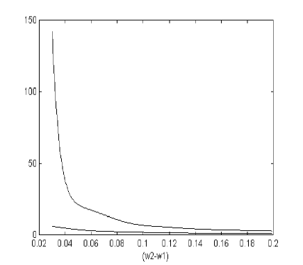
Figure 7: CRB and standard deviation of n.e. estimates; abscissa is the distance between the frequencies $\omega_{2}$ and $\omega_{1}$.
CRB (down); standard deviation of n.e. (up) with $m=5$, $\sigma=0.01$ and $M=20$.

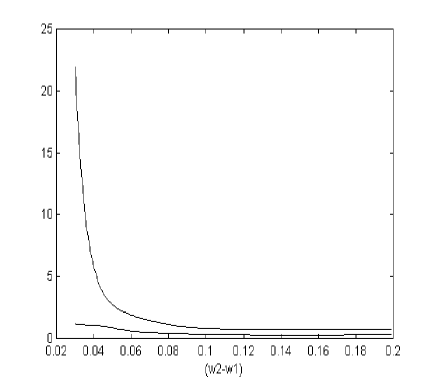
Figure 8: CRB and standard deviation of n.e. estimates; abscissa is the distance between the frequencies $\omega_{2}$ and $\omega_{1}$.
CRB (down); standard deviation of n.e. (up) with $m=5$, $\sigma=0.01$ and $M=20$.

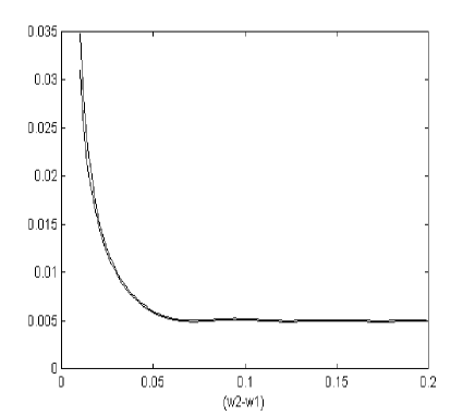
Figure 9: CRB and standard deviation of n.e. estimates; abscissa is the distance between the frequencies $\omega_{2}$ and $\omega_{1}$.
CRB (down); standard deviation of n.e. (up) with $m=20$, $\sigma=0.01$ and $M=100$.

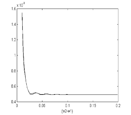
Figure 10: CRB and standard deviation of n.e. estimates; abscissa is the distance between the frequencies $\omega_{2}$ and $\omega_{1}$.
CRB (down); standard deviation of n.e. (up) with $m=50$, $\sigma=0.001$ and $M=100$.

Therefore, the n.e. estimate depends on both the increase of $m$ and the number of points in the input sequence. Increasing the number of points, we improve the estimate and the error approximates the Cramer-Rao bound. On the other hand, for noise variances very small, the estimate reaches a very good performance. Finally, we see that in all the experiments shown in the figures we reach the bound with a good approximation, and we can conclude that the n.e. method is statistically efficient.

7 Experimental results

7.1 Introduction

In this section we show the performance of the neural based estimator system using artificial and real data. The artificial data are generated following the literature (Kay 1988; Marple 1987) and are noisy sinusoidal mixtures. These are used to select the neural models for the next phases and to compare the n.e. with P’s, by using Montecarlo methods to generate samples. Real data, instead, come from astrophysics: in fact, real signals are light curves of Cepheids and a light curve in the Johnson’s system.

In the sections 7.3 and 7.4, we use an extension of Music to directly include unevenly sampled data without using the interpolation step of the previous algorithm in the following way:

$$P_{MUSIC}^{\prime}=\frac{1}{M-\sum_{i=1}^{p}|{\bf e}_{f}^{H}{\bf w}(i)|^{2}}$$ (23)

where $p$ is the frequency number, ${\bf w}(i)$ is the $i-$th weight vector of the PCA neural network after the learning, and ${\bf e}_{f}^{H}$ is the sinusoidal vector: ${\bf e}_{f}^{H}=[1,e_{f}^{j2\pi ft_{0}},\ldots,e_{f}^{j2\pi ft_{(L-1)}}]^{H}$ where $\left\{t_{0},t_{1},...,t_{\left(L-1\right)}\right\}$ are the first $L$ components of the temporal coordinates of the uneven signal.

Furthermore, to optimise the performance of the PCA neural networks, we stop the learning process when $\sum_{i=1}^{p}|{\bf e}_{f}^{H}{\bf w}(i)|^{2}>M\qquad\forall f$, so avoiding overfitting problems.

7.2 Models selection

In this section we use synthetic data to select the neural networks used in the next experiments. In this case, the uneven sampling is obtained by randomly deleting a fixed number of points from the synthetic sinusoid-mixtures: this is a widely used technique in the specialised literature (Horne & Baliunas 1986).

The experiments are organised in this way. First of all, we use synthetic unevenly sampled signals to compare the different neural algorithms in the neural estimator (n.e.) with the Scargle’s P.

For this type of experiments, we realise a statistical test using five synthetic signals. Each one is composed by the sum of five sinusoids of randomly chosen frequencies in $[0,0.5]$ and randomly chosen phases in $[0,2\pi]$ (Kay 1988; Karhunen & Joutsensalo 1994; Marple 1987), added to white random noise of fixed variance. We take $200$ samples of each signal and randomly discard $50\%$ of them ($100$ points), getting an uneven sampling (Horne & Baliunas 1986). In this way we have several degree of randomness: frequencies, phases, noise, deleted points.

After this, we interpolate the signal and evaluate the P and the n.e. system with the following neural algorithms: robust algorithm in equation(4) in the hierarchical and symmetric case; nonlinear algorithm in equation(8) in the hierarchical and symmetric case. Each of these is used with two nonlinear learning functions: $g_{1}(t)=\tanh(\alpha t)$ and $g_{2}(t)=sgn(t)\log(1+\alpha|t|)$. Therefore we have eight different neural algorithms to evaluate.

We chose these algorithms after we made several experiments involving all the neural algorithms presented in section 3, with several learning functions, and we verified that the behaviour of the algorithms and learning functions cited above was the same or better than the others. So we restricted the range of algorithms to better show the most relevant features of the test.

We evaluated the average differences between target and estimated frequencies. This was repeated for the five signals and then for each algorithm we made the average evaluation of the single results over the five signals. The less this averages were, the greatest the accuracy was.

We also calculated the average of the number of epochs and CPU time for convergence. We compare this with the behaviour of P.

Common signals parameters are: number of frequencies $=5$, variance noise $=0.5$, number of sampled points $=200$, number of deleted points $=100$.

Signal 1: frequencies=$0.03,0.19,0.25,0.33,0.46\quad 1/s$

Signal 2: frequencies=$0.02,0.11,0.20,0.33,0.41\quad 1/s$

Signal 3: frequencies=$0.34,0.29,0.48,0.42,0.04\quad 1/s$

Signal 4: frequencies=$0.32,0.20,0.45,0.38,0.13\quad 1/s$

Signal 5: frequencies=$0.02,0.37,0.16,0.49,0.31\quad 1/s$

Neural parameters: $\alpha=10.0$; $\mu=0.0001$; $\epsilon=0.001$; number of points in each pattern $N=110$ (these are used for almost all the neural algorithms; however, for a few of them a little variation of some parameters is required to achieve convergence).

Scargle parameters: $Tapering=30\%$, $p_{0}=0.01$.

Results are shown in Table 1:

Table 1: Performance evaluation of n.e. algorithms and P on synthetic signals.

	average normalised differences
Algorithm	sig1	sig2	sig3	sig4	sig5	TOT	average	average
							n. epochs	time
1. eq.(4) hierarc.+$g1$	0.000	0.002	0.004	0.000	0.004	0.0020	898.4	189.2 s
2. eq.(4) hierarc.+$g2$	0.000	0.002	0.004	0.000	0.004	0.0020	667.2	105.2 s
3. eq.(8) hierarc.+$g1$	0.000	0.002	0.005	0.000	0.004	0.0022	5616.2	1367.4 s
4. eq.(8) hierarc.+$g2$	0.000	0.002	0.005	0.000	0.004	0.0022	3428.4	1033.4 s
5. eq.(4) symmetr.+$g1$	0.000	0.002	0.002	0.000	0.004	0.0016	814.0	100.2 s
6. eq.(4) symmetr.+$g2$	0.000	0.002	0.004	0.002	0.004	0.0024	855.2	124.4 s
7. eq.(8) symmetr.+$g1$	0.000	0.002	0.004	0.002	0.004	0.0024	6858.2	1185 s
8. eq.(8) symmetr.+$g2$	0.000	0.002	0.004	0.002	0.004	0.0024	3121.8	675.8 s
Periodogram	0.004	0.000	0.002	0.004	0.004	0.0028		22.2 s

We have to spend few words about the differences of behaviour among the neural algorithms elicited by the experiments. Nonlinear algorithms are more complex than robust ones; they are relatively slower in converging, with higher probability to be caught in local minima, so their estimates results are sometimes not reliable. So we restrict our choice to robust models. Moreover, symmetric models require more effort in finding the right parameters to achieve convergence than the hierarchical ones. The performance, however, are comparable.

From Table 1 we can see that the best neural algorithm for our aim is the n.5 in Table 1 (equation(4) in the symmetric case with learning function $g_{1}(t)=\tanh(\alpha t)$).

However, this algorithm requires much more efforts in finding the right parameters for the convergence than the algorithm n.2 from the same table (equation(4) in the hierarchical case with learning function $g_{2}(t)=sgn(t)\log(1+\alpha|t|)$), which has performance comparable with it.

For this reason, in the following experiments when we present the neural algorithm, it is algorithm n.2.

We show, as an example, in figures 11-13 the estimate result of the n.e. algorithm and P on signal n.1.

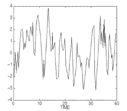
Figure 11: Synthetic Signal.

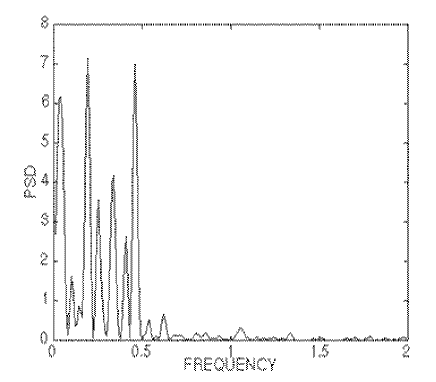
Figure 12: P estimate.

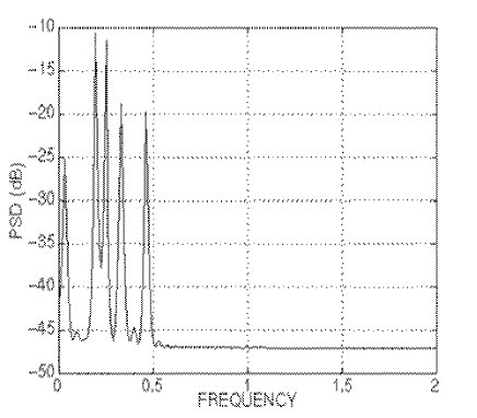
Figure 13: n.e. estimate.

We now present the result for whitening pre-processing on one synthetic signal (figures 14-16). We compare this technique with the standard n.e. .

Signal frequencies=$0.1,0.15,0.2,0.25,0.3\quad 1/s$

Neural network estimates with whitening: $0.1,0.15,0.2,0.25,0.3\quad 1/s$

Neural network estimates without whitening: $0.1,0.15,0.2,0.25,0.3\quad 1/s$

From this and other experiments we saw that when we used the whitening in our n.e. the results were worse and more time consuming than the ones obtained using the standard n.e. (i.e. without whitening the signal). For these reasons whitening is not a suitable technique to improve our n.e. .

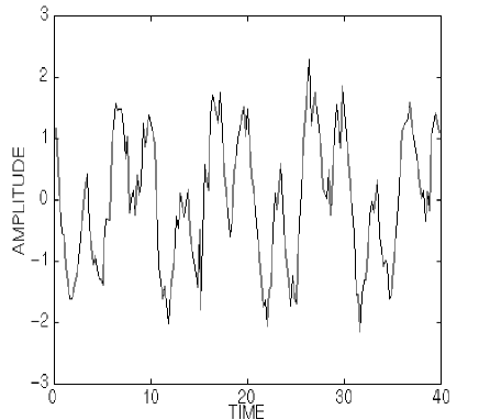
Figure 14: Synthetic Signal.

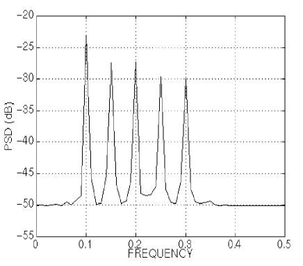
Figure 15: n.e. estimate without whitening.

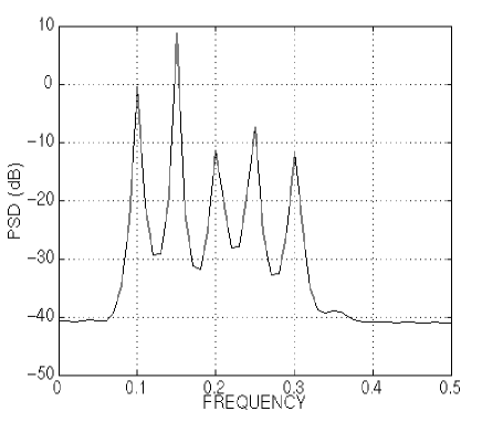
Figure 16: n.e. estimate with withening.

7.3 Comparison of the n.e. with the Lomb’s Periodogram

Here we present a set of synthetic signals generated by random varying the noise variance, the phase and the deleted points with Montecarlo methods. The signal is a sinusoid ($0.5\cos(2\pi 0.1t+\phi)+R(t)$) with frequency $0.1$ $Hz$, $R(t)$ the Gaussian random noise with $0$ mean composed by $100$ points, with a random phase. We follow Horne & Baliunas (Horne & Baliunas 1986) for the choice of the signals.

We generated two different series of samples depending on the number of deleted points: the first one with $50$ deleted points, the second one with $80$ deleted points. We made 100 experiments for each variance value. The results are shown in Table 2 and Table 3, and compared with the Lomb’s P because it works better than the Scargle’s P with unevenly spaced data, introducing confidence intervals which are useful to identify the accepted peaks.

The results show that both the techniques obtain a comparable performance.

Table 2: Synthetic signal with 50 deleted points, frequency interval $\left[\frac{2\pi}{T},\frac{\pi N_{o}}{T}\right]$, MSE = Mean Square Error, $T$ = total period $(X_{max}-X_{min})$ and $N_{o}$ = total number of points.

		Lomb’s P			n.e.
Error Variance $\sigma^{2}$	S.N.R. $\xi=\frac{X_{o}}{2\sigma^{2}}$	Mean	Variance	MSE	Mean	Variance	MSE
0.75	0.2	0.1627	0.0140	0.0178	0.1472	0.0116	0.0131
0.5	0.5	0.1036	0.0013	0.0013	0.1020	3.0630 e-4	3.0725 e-4
0.1	12.5	0.1000	1.0227 e-8	1.0226 e-8	0.1000	6.1016 e-8	6.2055 e-8
0.001	1250	0.1000	2.905 e-9	2.3139 e-9	0.1000	3.8130 e-32	0.00000

Table 3: Synthetic signal with 80 deleted points, frequency interval $\left[\frac{2\pi}{T},\frac{\pi N_{o}}{T}\right]$, MSE = Mean Square Error, $T$ = total period $(X_{max}-X_{min})$ and $N_{o}$ = total number of points.

		Lomb’s P			n.e.
Error Variance $\sigma^{2}$	S.N.R. $\xi=\frac{X_{o}}{2\sigma^{2}}$	Mean	Variance	MSE	Mean	Variance	MSE
0.75	0.2	0.2323	0.0205	0.0378	0.2055	0.0228	0.0337
0.5	0.5	0.2000	0.0190	0.0288	0.2034	0.0245	0.0349
0.1	12.5	0.1000	2.37 e-7	2.3648 e-7	0.1004	1.8437 e-5	1.8435 e-5
0.001	1250	0.1000	8.6517 e-8	8.5931 e-8	0.1000	4.7259 e-8	4.7259 e-8

7.4 Real data

The first real signal is related to the Cepheid SU Cygni (Fernie 1979). The sequence was obtained with the photometric tecnique UBVRI and the sampling made from June to December 1977. The light curve is composed by 21 samples in the V band, and a period of $3.8^{d}$, as shown in figure 17. In this case, the parameters of the n.e. are: $N=10$, $p=2$, $\alpha=20$, $\mu=0.001$. The estimate frequency interval is $\left[0(1/JD),0.5(1/JD)\right]$. The estimated frequency is $0.26$ (1/JD) in agreement with the Lomb’s P, but without showing any spurious peak (see figures 18 and 19).

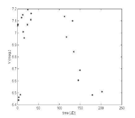
Figure 17: Light curve of SU Cygni.

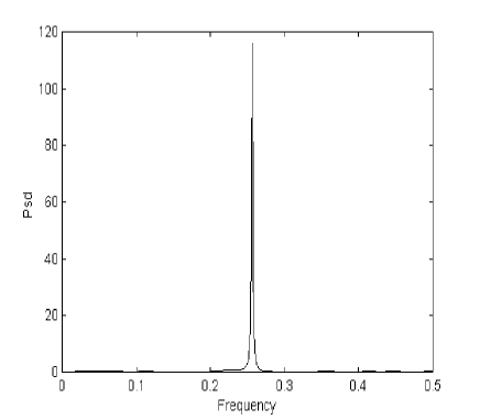
Figure 18: n.e. estimate of SU Cygni.

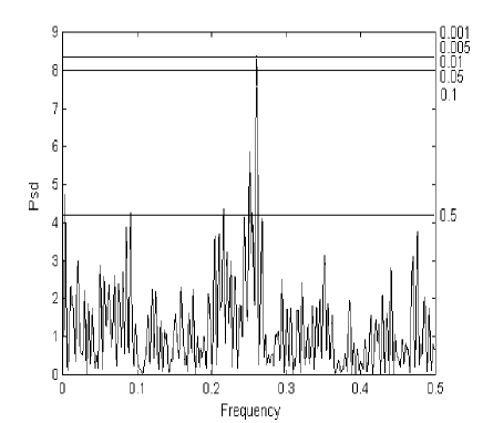
Figure 19: Lomb’s P estimate of SU Cygni.

The second real signal is related to the Cepheid U Aql (Moffet and Barnes 1980). The sequence was obtained with the photometric tecnique BVRI and the sampling made from April 1977 to December 1979. The light curve is composed by 39 samples in the V band, and a period of $7.01^{d}$, as shown in figure 20. In this case, the parameters of the n.e. are: $N=20$, $p=2$, $\alpha=5$, $\mu=0.001$. The estimate frequency interval is $\left[0(1/JD),0.5(1/JD)\right]$. The estimated frequency is $0.1425$ (1/JD) in agreement with the Lomb’s P, but without showing any spurious peak (see figures 21 and 22).

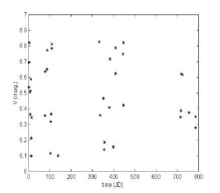
Figure 20: Light curve of U Aql.

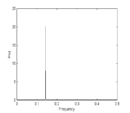
Figure 21: n.e. estimate of U Aql.

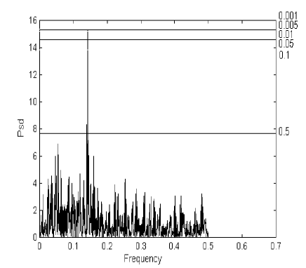
Figure 22: Lomb’s P estimate of U Aql.

The third real signal is related to the Cepheid X Cygni (Moffet and Barnes 1980). The sequence was obtained with the photometric technique BVRI and the sampling made from April 1977 to December 1979. The light curve is composed by 120 samples in the V band, and a period of $16.38^{d}$, as shown in figure 23. In this case, the parameters of the n.e. are: $N=70$, $p=2$, $\alpha=5$, $\mu=0.001$. The estimate frequency interval is $\left[0(1/JD),0.5(1/JD)\right]$. The estimated frequency is $0.061$ (1/JD) in agreement with the Lomb’s P, but without showing any spurious peak (see figures 24 and 25).

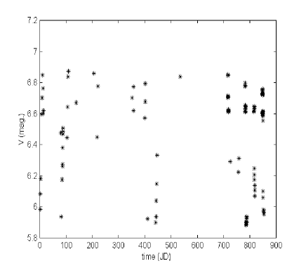
Figure 23: Light curve of X Cygni.

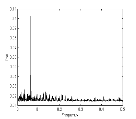
Figure 24: n.e. estimate of X Cygni.

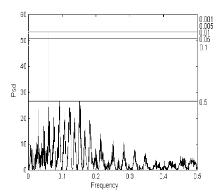
Figure 25: Lomb’s P estimate of X Cygni.

The fourth real signal is related to the Cepheid T Mon (Moffet and Barnes 1980). The sequence was obtained with the photometric technique BVRI and the sampling made from April 1977 to December 1979. The light curve is composed by $24$ samples in the V band, and a period of $27.02^{d}$, as shown in figure 26. In this case, the parameters of the n.e. are: $N=10$, $p=2$, $\alpha=5$, $\mu=0.001$. The estimate frequency interval is $\left[0(1/JD),0.5(1/JD)\right]$. The estimated frequency is $0.037$ (1/JD) (see figure 28).

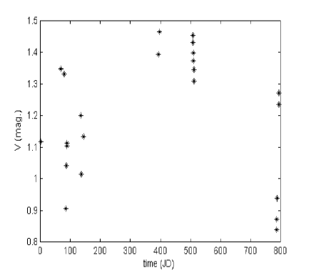
Figure 26: Light curve of T Mon.

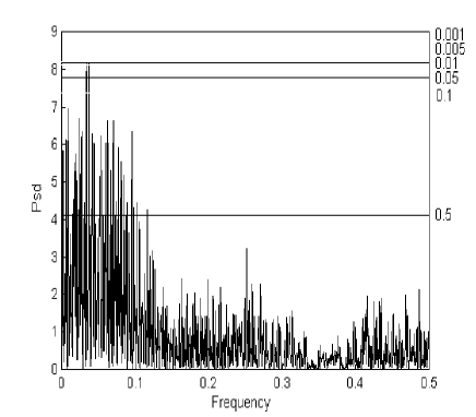
Figure 27: Lomb’s P estimate of T Mon.

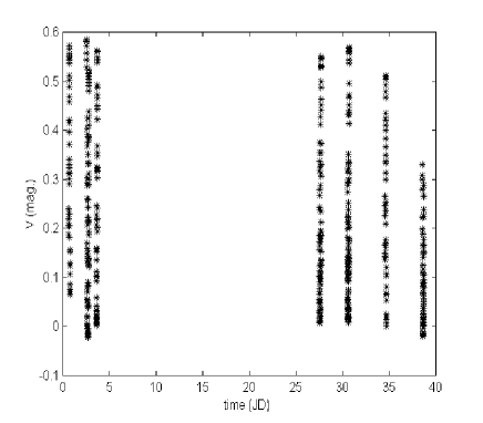
Figure 28: n.e. estimate of T Mon.

The Lomb’s P does not work in this case because there many peaks, and at least two greater than the threshold of the most accurate confidence interval (see figure 27).

The fifth real signal we used for the test phase is a light curve in the Johnson’s system (Binnendijk 1960) for the eclipsing binary U Peg (see figure 29 and 30). This system was observed photoelectrically in the effective wavelengths 5300 A and 4420 A with the 28-inch reflecting telescope of the Flower and Cook Observatory during October and November, 1958.

Figure 29: Light curve of U Peg.

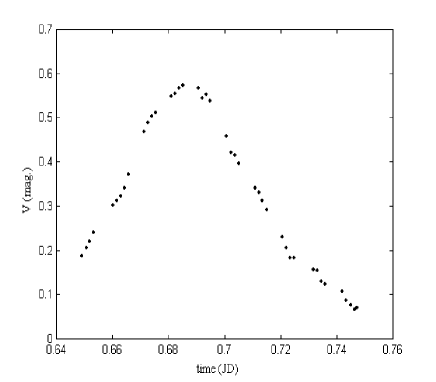
Figure 30: Light curve of U Peg (first window).

We made several experiments with the n.e., and we elicited a dependence of the frequency estimate on the variation of the number of elements for input pattern. The optimal experimental parameters for the n.e. are: $N=300$, $\alpha=5$; $\mu=0.001$. The period found by the n.e. is expressed in $JD$ and is not in agreement with results cited in literature (Binnendijk 1960), (Rigterink 1972), (Zhai et al. 1984),(Lu 1985) and (Zhai et al. 1988). The fundamental frequency is $5.4$ $1/JD$ (see figure 31) instead of $2.7$ $1/JD$. We obtain a frequency double of the observed one. Lomb’s P has some high peaks as in the previous experiments and the estimated frequency is always the double of the observed one (see figure 32).

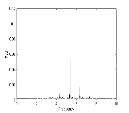
Figure 31: n.e. estimate of U Peg.

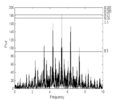
Figure 32: Lomb’s P of U Peg.

8 Conclusions

We have realised and experimented a new method for spectral analysis for unevenly sampled signals based on three phases: preprocessing, extraction of principal eigenvectors and estimate of signal frequencies. This is done, respectively, by input normalization, nonlinear PCA neural networks, and the Multiple Signal Classificator algorithm. First of all, we have shown that neural networks are a valid tool for spectral analysis.

However, above all, what is really important is that neural networks, as realised in our neural estimator system, represent a new tool to face and solve a problem tied with data acquisition in many scientific fields: the unevenly sampling scheme.

Experimental results have shown the validity of our method as an alternative to Periodogram, and in general to classical spectral analysis, mainly in presence of few input data, few a priori information and high error probability. Moreover, for unevenly sampled data, our system offers great advantages with respect to P. First of all, it allows us to use a simple and direct way to solve the problem as shown in all the experiments with synthetic and Cepheid’s real signals. Secondly, it is insensitive to the frequency interval: for example, if we expand our interval in the SU Cygni light curve, while our system finds the correct frequency, the Lomb’s P finds many spurious frequencies, some of them greater than the confidence threshold, as shown in figures 33 and 34.

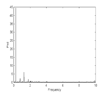
Figure 33: n.e. estimate of SU Cygni with enlarged window.

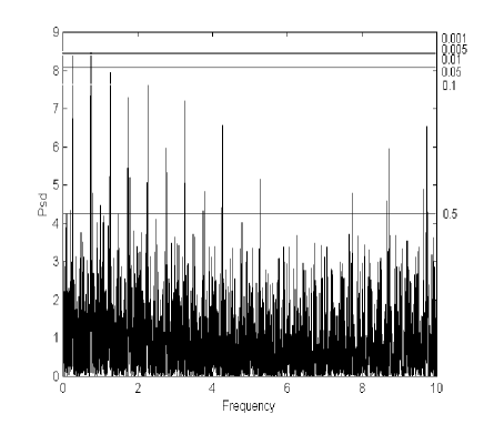
Figure 34: Lomb’s P of SU Cygni with enlarged window.

Furthermore, when we have a multifrequency signal, we can use our system also if we do not know the frequency number. In fact, we can detect one frequency at each time and continue the processing after the cancellation of the detected periodicity by IIR filtering.

A point worth of noting is the failure to find the right frequency in the case of eclipsing binary for both our method and Lomb’s P. Taking account of the morphology of eclipsing light curve with two minima, this fact can not be of concern because in practical cases the important thing is to have a first guess of the orbital frequency. Further refinement will be possible through a wise planning of observations. In any case we have under study this point to try to find a method to solve the problem.

References

- (1) Baldi P., Hornik K., 1989, Neural Networks 2, 53
- (2) Barone F., Milano L., Russo G., 1994, ApJ 421, 284
- (3) Binnendijk L., 1960, AJ 65, 88
- (4) Brescia M., D’Argenio B., Longo G., Pelosi S., Tagliaferri R., 1996, Earth Planetary Science and Letters 139, 33
- (5) Deeming T. J., 1975, Ap&SS 36, 137
- (6) Ferraz-Mello S., 1981, AJ, 86, 619
- (7) Fernie J. D., 1979, PASP 91, 67
- (8) Jutten C., Herault J., 1991, Signal Processing 24, 1
- (9) Horne J. H., Baliunas S. L., 1986, ApJ 302 757
- (10) Horowitz L. L., IEEE Trans., ASSP-22, 22, 1974.
- (11) Karhunen J., Joutsensalo J., 1994, Neural Networks 7, 113
- (12) Karhunen J., Joutsensalo J., 1995, Neural Networks, 8, 549
- (13) Kay S. M., 1988, Modern spectral estimation: theory and application. Prentice-Hall, Englewood Cliffs, N. Y.
- (14) Lomb N. R., 1976, Ap&SS 39, 447
- (15) Lu W., 1985, PASP 97, 1086
- (16) Marple S. L., 1987, Digital spectral analysis with applications. Prentice-Hall, Englewood Cliffs, N. Y.
- (17) Moffet T. J., Barnes T. G., 1980, ApJS 44, 427
- (18) Numerical Recipes in C: The Art of Scientific Computing. 1988-1992, Cambridge University Press , Cambridge, p.575 http://www.nr.com
- (19) Oja E., 1982, Journal of Mathematical Biology, 15, 267
- (20) Oja E., Ogawa H., Wangviwattana J., 1991, Learning in nonlinear constrained Hebbian network. In T. Kohonen et al. (Eds.), Artificial neural networks, North-Holland, Amsterdam, p. 385
- (21) Oja E., Karhunen J., Wang L., Vigario R., 1996, Principal and independent components in neural networks - recent developments. In Marinaro M., Tagliaferri R. (eds), WIRN Vietri ’95,World Scientific Pu., Singapore, p. 16-35
- (22) Oppenheim A. V., Schafer R. W., 1965, Digital signal processing. Prentice-Hall, N.Y.
- (23) Plumbley M., 1993, A Hebbian/anti Hebbian network which optimizes information capacity by orthonormalizing the principal subspace. In J. Taylor et. al (eds) Proc. Int. Conf. on Artificial Neural Networks, p. 86
- (24) Rigterink P. V., 1972, AJ 77, 319
- (25) Sanger T. D., 1989, 2, 459
- (26) Scargle J. D., 1982, ApJ 263, 835
- (27) Stoica P., Nehorai A., 1990 IEEE Transactions on Acoustics, Speech, and Signal Processing, 38, 12
- (28) Wilson R. E., Devinney E. J., 1971, ApJ 166, 605
- (29) Zhai, D. S., Leung K. C., Zhang R. X., 1984, A&AS 57, 487
- (30) Zhai, D. S., Lu W.X., Zhang X. Y., 1988, Ap&SS 146, 1