A Method of Mass Measurement in Black Hole Binaries
Using Timing and High Resolution X-ray Spectroscopy

Abstract

In X-ray binaries, several percent of the compact object luminosity is intercepted by the surface of the normal companion and re-radiated through Compton reflection and the K-fluorescence. This reflected emission follows the variability of the compact object with a delay approximately equal to the orbital radius divided by the speed of light. This provides the possibility of measuring the orbital radius and thus substantially refining the compact object mass determination compared to using optical data alone. We demonstrate that it may be feasible to measure the time delay between the direct and reflected emission using cross-correlation of the light curves observed near the K line and above the K-edge of neutral iron. In the case of Cyg X-1, the time delay measurement is feasible with a $3\times 10^{5}-10^{6}\,$s observation by a telescope with a 1000 cm² effective area near 6.4 keV and with a $\sim 5\,$eV energy resolution. With longer exposures, it may be possible to obtain mass constraints even if an X-ray source in the binary system lacks an optical counterpart.

1. Introduction

The existence of stellar-mass black holes in our Galaxy is almost exclusively established by measuring the mass of the compact object in several bright X-ray binaries. A compact object more massive than approximately $3\,M_{\odot}$ is unstable and should collapse to form a black hole (Rhoades & Ruffini 1974, Chitre & Hartle 1976). Therefore, if the dynamically measured mass of a luminous X-ray source exceeds $3\,M_{\odot}$, it is considered a firm black hole candidate.

In X-ray binaries, the orbital velocity of the compact object cannot be measured by means of optical spectroscopy. This means that the only directly measured quantity is the mass function $f(M)$,

$$f(M)=\frac{M_{x}^{3}\sin^{3}i}{(M_{x}+M_{\rm opt})^{2}},$$ (1)

where $M_{x}$ and $M_{\rm opt}$ are masses of the compact object and normal companion, respectively, and $i$ is the inclination angle of the orbit. The mass function is the lower limit of the compact object mass. In many high mass X-ray binaries, the mass function is uninterestingly low; for example, $f(M)=0.25\,M_{\odot}$ for Cyg X-1 (Gies & Bolton 1986). A determination of $M_{x}$ is possible if $M_{\rm opt}$ and $\sin i$ are independently constrained. Extensive work has been done to estimate these parameters for several black hole candidates (Bolton 1972, Liutyj, Sunyaev & Cherepashchuk 1975, McClintock & Remillard 1986, Remillard, McClintock & Bailyn 1992, Herrero et al. 1995, Filippenko, Matheson & Barth 1995, Bailyn et al. 1995, Remillard et al. 1996). However, the derived compact object mass can be rather uncertain due to its strong dependence on $M_{\rm opt}$ and especially $\sin i$. For Cyg X-1, mass values in the range 6–16$\,M_{\odot}$ are found in the literature (Dolan & Tapia 1989, Gies & Bolton 1986).

The mass measurement will be much more accurate if some information about the orbit of the compact object is available. Unfortunately, very fast motions of the material in the vicinity of the black hole make it impossible to measure the orbital velocity from the Doppler shifts of spectral lines. Instead, we propose to measure the orbital radius using the following approach. In high mass X-ray binaries, some fraction of the compact object X-ray luminosity is intercepted by the normal companion surface (the intercepted fraction in low mass binaries is too low for an application of our method). A significant fraction of this energy is re-radiated in the X-ray band either through Compton reflection or line fluorescence. This emission reaches the observer with a time delay roughly equal to $a/c$, where $a$ is the separation between the normal companion and the compact object. Since the compact object emission is usually variable, it may be possible to measure the time delay and thus estimate the orbital radius. We show below that this measurement can be carried out using temporally resolved high resolution spectroscopy of the fluorescent K line of neutral iron. Let us demonstrate how this new information refines the measurement of the compact object mass. Suppose for simplicity that the orbit is circular and the radius of the normal companion is negligible compared to the orbital radius. The time delay at orbital phase $\phi$ is

$$\Delta t=a/c\left[1-\sin(i\,\cos 2\pi\phi)\right].$$ (2)

Equations (1)–(2) together with the Kepler’s third law,

$$a^{3}=P^{2}(M_{x}+M_{\rm opt})G/4\pi^{2},$$ (3)

can be used to express $M_{x}$ as a function of just one parameter, $M_{\rm opt}$, $i$, or $a$. In particular, if the time delay measurement is performed at inferior conjunction ($\phi=0.5$),

$$M_{x}=\frac{f^{1/3}\;g^{2/3}}{\sin i\;(1+\sin i)^{2}}\quad{\rm or}\quad M_{x}=\frac{(M_{x}+M_{\rm opt})f^{1/3}}{g^{1/3}-(M_{x}+M_{\rm opt})^{1/3}},$$ (4)

where $g=4\pi^{2}(c\Delta t)^{3}/P^{2}G$. If the time delay is measured at several orbital phases, all system parameters can be determined independently. Moreover, useful mass constraints are possible in this case even if no optical data are available (§ 4).

2. Measurement strategy

The X-ray emission reflected from the surface of the normal companion consists of the Compton-reflected continuum and the fluorescent emission. While the reflected continuum is weak compared to the direct emission from the black hole, the fluorescent line emission can be relatively strong. The strongest fluorescent line is the iron K doublet (Basko, Sunyaev & Titarchuk 1974). Basko (1978) estimates the equivalent width of $\approx 7\,$eV for this line in Cyg X-1. With $\approx 5\,$eV spectral resolution of X-ray calorimeters, it should be possible to measure the source light curve in a narrow spectral interval around K₁ and K₂, where the fluorescent line contributes $\approx 50\%$ of the total flux. The time delay can be measured by cross-correlating the light curve in the K region with the continuum light curve which is dominated by the direct black hole emission.

K lines are primarily excited through photoelectric absorption in the K-edge ($E_{K}=7.1$ keV for neutral iron). Therefore, the energy band just above 7.1 keV is best for the continuum light curve measurement. The exact choice of the energy boundaries is unimportant as long as the source variability patterns do not change with energy, as is the case in Cyg X-1 (Nowak et al. 1999). Below, we assume that the continuum is measured in the 7.1–9.1 keV energy band.

The most challenging part of the time delay measurement is determining the light curve in the K line region. This line consists of two components, K₁ and K₂, with energies $E_{{}_{1}}=6.404$ and $E_{{}_{2}}=6.391$ keV (Bambynek et al. 1972). Both components have approximately equal natural widths of 3.5 eV (FWHM). The Doppler broadening of the lines due to thermal motions of the emitting atoms $\Delta E_{\rm th}=0.1\,(T/10^{5}\,{\rm K})^{1/2}$ eV is much smaller than the natural width of the lines. Therefore, more than 90% of the total K line flux is within a narrow, 20 eV, energy interval around $E=6.398$ keV. Selecting photons in this energy interval is easy with the 5 eV (FWHM) energy resolution of future X-ray calorimeters. An approximately 20 eV energy interval seems optimal for the time delay measurement. A wider band would include a larger contribution of the direct continuum without increasing the line flux significantly. Narrower intervals would miss flux in the line wings.

The cross-correlation function of the continuum and line light curves should contain two prominent peaks. A strong narrow peak around the delay $\tau=0$ corresponds to the auto-correlation of the emission coming directly from the black hole. Reflection from the normal companion results in a secondary broad peak in the correlation function. This peak should have a centroid at $\tau\approx-a/c$ and width $\Delta\tau\approx R/c$, where $a$ and $R$ are the radii of the orbit and normal companion, respectively. The amplitude of the secondary peak should be proportional to the equivalent width of the reflected K line and the ${\it rms}^{2}$ of the source flux variability. Therefore, the time delay measurement is best performed when the reflected line is strong (i.e. near inferior conjunction, Basko 1978), and when the source is highly variable.

In the next section, we simulate an observation of the time delay in Cyg X-1 which could be performed by a telescope with an effective area of 1000 cm² in the 6–9 keV energy range. Such an instrument approximately corresponds to one spacecraft of the proposed Constellation-X mission.

3. Simulated Observation

We adapt the binary system parameters from Herrero et al. (1995) — a radius of the normal companion $R=17\,R_{\odot}$, a separation between the components $a=40\,R_{\odot}$, and an inclination angle $i=35^{\circ}$. For simplicity, we assume that the orbit is circular and the normal companion is spherical. For a similar geometry, Basko (1978) predicted the equivalent width of the reflected iron line at inferior conjunction $W_{\phi=0.5}=7$ eV. Basko assumed Solar chemical composition of the normal companion. However, some X-ray observations indicate that the iron abundance may be twice Solar (Kitamoto et al. 1984). Such an overabundance of iron would increase the fluorescent line flux to $W\approx 14$ eV. A narrow iron K line of similar amplitude was indeed observed by the ASCA SIS (Ebisawa et al. 1996). We adopt $W_{\phi=0.5}=10\,$eV, which agrees with both theoretical predictions and current observations.

As was discussed in § 2, we assume that the K light curve is measured in the 20 eV energy interval centered at $6.398$ keV, and the continuum light curve is observed in the 7.1–9.1 keV band. The continuum spectrum is assumed to be a power law with a photon index $\Gamma=1.65$ (Liang & Nolan 1984). We also allow for the possible presence of a broad iron line originating in the vicinity of the black hole, for example, in the outer part of the accretion disk. We assume that the equivalent width of the broad line is 0.1 keV (see, e.g., Dove et al. 1998) and that the line width is 0.08 keV (FWHM) which corresponds to the velocity dispersion of 2000 km s^-1.

For the source variability, we adopt the shot noise model of Lochner et al. (1991). This model describes the variability of Cyg X-1 as a constant component plus a sequence of exponential flares with durations distributed in the 0.01–3.22 s interval. The variability level during the 1997 HEAO 1 A-2 observation modeled by Lochner et al. was quite typical of the source (35% rms). The shot noise model is adequate for simulation of the direct emission from the black hole. The light curve of the reflected radiation is the convolution of the direct emission light curve with the reflection response to the instantaneous flare. This response function is calculated below.

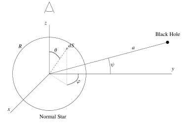
Figure 1.— Geometry of the reflection problem. The line of sight is along the $z$-axis. Black hole is in the $y-z$ plane; $\psi=-i\cos 2\pi\phi$, where $\phi$ is the orbital phase.

Figure 2.— Time response of the fluorescent emission in the Cyg X-1 system ($R/c=40\,$s and $a/c=93\,$s in this case).

Figure 3.— The cross-correlation analysis of simulated 1000 ks observations of Cyg X-1 at three orbital phases. Correlation functions for $\phi=0.5$ and $\phi=0$ are offset for clarity by $0.003$ and $-0.003$, respectively.

Consider the fluorescent emission coming to the observer from the normal companion surface element $dS$ (Fig. 3). The distance between the surface element and the black hole is

$$l=\left[R^{2}+a^{2}-2Ra\,(\cos\psi\sin\theta\cos\varphi+\sin\psi\cos\theta)\right]^{1/2}.$$ (5)

The reflected emission reaches the observer with a delay $\tau$

$$c\tau=l+a\sin\psi-R\cos\theta$$ (6)

relative to the direct emission from the black hole. The fraction of the X-ray luminosity intercepted by the surface element is

$$dL=L\;dS\,\cos\Theta_{i}/4\pi l^{2},$$ (7)

where $\Theta_{i}$ is the incident angle of the X-rays,

$$\cos\Theta_{i}=(\cos\psi\sin\theta\cos\varphi+\sin\psi\cos\theta)\,a/l-R/d.$$ (8)

The ratio of intensities of the observed K line and the incident continuum above the K-edge is a strong function of $\Theta_{i}$ and the fluorescence angle, $\theta$. This ratio, $Y(\Theta_{i},\theta)$, can be calculated analytically following the work of Basko. It was also derived by George & Fabian (1991) using Monte-Carlo simulations. George & Fabian present $Y(\Theta_{i},\theta)$ for an incident power-law spectrum with $\Gamma=1.7$ on a grid of $\Theta_{i}$ and $\theta$ values. We use numerical interpolation of the George & Fabian results in our calculations below.

The light curve of the fluorescent emission from the surface element is

$$f(t)=Y(\Theta_{i},\theta)\;\delta(t-\tau)\;dL$$ (9)

Integration of equation (9) over the normal companion’s surface provides the time response of the reflected emission. Figure 3 shows the results for the Cyg X-1 system at three orbital phases. A different set of responses is expected for a non-spherical normal companion, for example, the one filling its Roche lobe. However, the calculations in this case should be analogous to the procedure outlined above.

Our simulations proceed as follows. The continuum light curve in the 7.1–9.1 keV band is simulated using the shot noise model of Lochner et al. The reflected K line light curve is the convolution of the 7.1–9.1 keV light curve with the time response from Fig 3. The K line flux is rescaled so that the line equivalent width (relative to the $\Gamma=1.65$ power law continuum) is 10 eV at $\phi=0.5$. The 6.388–6.408 keV flux as a sum of the K line flux and the contribution of the direct emission calculated as the 7.1–9.1 keV light curve scaled according to the spectral model which consists of the power law and a broad 6.4 keV line (see above). Finally, we scale the simulated light curves to reproduce the observed Cyg X-1 flux at 7 keV (0.05 ph s^-1 cm^-2 keV^-1, Ebisawa et al. 1996), multiply them by the effective area of 1000 cm², and add Poisson noise.

The cross-correlation functions derived from the simulated $1000\,$ksec observations are presented in Fig 3. The secondary peak due to reflected emission is clearly visible at orbital phases $\phi=0.5$ and 0.25. For $\phi=0$, the secondary cross-correlation peak is weak and not separated from the autocorrelation of the direct emission (the average delay is only 14 s for the adopted system parameters).

4. Discussion

We have shown that the time delay between the direct and reflected emission can be measured in a Cyg X-1 like system. Arguably, this measurement requires long observations. For a convincing detection, a 250 ksec observation on a telescope with 1000 cm² effective area around 6 keV is required. A longer, 1000 ksec, exposure is needed for a quality measurement of the cross-correlation function (Fig 3). These exposures are longer than the 5.6 day orbital period of Cyg X-1, and therefore the observation needs to be split into several intervals, each performed at the same orbital phase. The required exposure is shorter for larger area telescopes. Unfortunately, the gain is smaller than a factor of $({\rm area})^{1/2}$ because the internal source variability becomes the dominant source of noise. To achieve a detection significance similar to that in Fig. 3, $\approx 300$ ksec exposure is a minimum even for very large area telescopes.

In addition to the fluorescence from the surface of the normal companion, iron K lines can form in the accretion disk or stellar wind. These emissions are contaminants for the time delay measurement. Fortunately, it may be possible to separate them in the energy or time domains from the normal component fluorescence. First, lines originating in the accretion disk or stellar wind are likely to be significantly broadened because the reflecting material moves at high speed (a possible detection of the broadened iron line in Cyg X-1 is reported by Done & Zycki 1999). Thus, we can exclude a large fraction of the disk and possibly wind fluorescent emission by selecting a narrow range around the K line rest frame energy. Second, iron in both wind and disk is likely to be partially ionized because of the low matter density and high ionizing flux from the black hole. K lines for ionization states higher than ${\rm Fe}\,{\rm XV}$ are separated from the ${\rm Fe}\,{\rm I}$ lines by more than 20 eV (House 1969). Third, the accretion disk or stellar wind fluorescence should produce cross-correlation functions very different from those in Fig. 3. Since the outer disk radius is only a small fraction of the black hole Roche lobe size (Shapiro & Lightman 1976), the time delay of the fluorescent disk emission is much shorter than that in Fig. 3. In the case of stellar wind fluorescence, time delays should be distributed in the broad range $\Delta\tau\approx r/c$ around the average value $\overline{\tau}=r/c$, where $r$ is the characteristic radius of the fluorescence region. Therefore, a very broad feature in the cross-correlation function is expected due to stellar wind fluorescence. Such a feature should be easily distinguishable from the relatively narrow peak arising from the normal companion reflection. To conclude, the only consequence of the presence of the iron K-fluorescence from the stellar wind or accretion disk is to add noise to the cross-correlation function in the time delay range of interest.

The quality of the data in our simulated observation is sufficient to determine both the average delay and shape of the cross-correlation peak. The average delay provides the orbital separation between the components which can be used to refine the black hole mass estimates (§ 1). The width of the correlation peak is proportional to the radius of the normal companion. Its shape depends on the shape of the companion surface and the inclination angle (e.g., the $\phi=0.25$ curve in Fig. 3 corresponds to all orbital phases in an $i=0$ system). The shift of the average delay as a function of the orbital phase also depends on the inclination angle and the companion radius (eq. 2, Fig. 3). Therefore, a much more detailed modeling than simple considerations outlined in eqs. (2)–(4) might be possible with high-quality time delay data. This should result in the compact object mass determination without the $\sin i$ or $M_{\rm opt}$ degeneracies of eq (4).

Basko (1978) pointed out that the orbital modulation of the reflected K line flux can be used to estimate the orbital parameters, in particular, the inclination angle. Our method is independent of Basko’s, because we do not use the line flux. The interpretation of the orbital modulation of the K line flux can be uncertain. For example, the fluorescence in the stellar wind reduces the orbital modulation of the line flux; a similar behavior is expected for low inclination angles (see Basko’s Fig. 4). On the contrary, our method is not directly affected by either stellar wind or accretion disk fluorescence.

The time delay technique opens the possibility of mass determination in X-ray systems without known optical counterparts, such as bright black hole candidates in the Galactic center region or LMC. In these systems, the binary period and the epoch of zero orbital phase can be determined by periodic variations of either the iron line intensity (Basko 1978) or location of the cross-correlation peak. Near the orbital phase $\phi=0.25$, the cross-correlation function is independent of the inclination angle and can be used to measure the orbital radius, $a$, and the radius of the normal companion, $R$, (Fig. 3). The total system mass $M_{\rm opt}+M_{x}$ is then determined from the Kepler’s third law. Under the assumption that the normal companion almost fills its Roche lobe, which should be the case in X-ray luminous systems, the ratio $R/a$ defines $M_{x}/M_{\rm opt}$ and thus provides an estimate of $M_{x}$.

References

- (1)
- (2) Bailyn, C. D., Orosz, J. A., McClintock, J. E., & Remillard, R. A. 1995, Nature, 378, 157
- (3)
- (4) Bambynek, W., Craseman, B., Fink, R. W., Freund, H. U., Mark, H., Swift, C. D., Price, R. E., & Rao, P. V. 1972, Rev. Mod. Phys., 44, 716
- (5)
- (6) Basko, M. M. 1978, ApJ, 223, 268
- (7)
- (8) Basko, M. M., Sunyaev, R. A., & Titarchuk, L. G. 1974, A&A, 31, 249
- (9)
- (10) Bolton, C. T. 1972, Nature, 235, 271
- (11)
- (12) Chitre, D. M. & Hartle, J. B. 1976, ApJ, 207, 592
- (13)
- (14) Dolan, J. F. & Tapia, S. 1989, ApJ, 344, 830
- (15)
- (16) Done, C. & Zycki, P. T. 1999, MNRAS, 305, 457
- (17)
- (18) Dove, J. B., Wilms, J., Nowak, M. A., Vaughan, B. A., & Begelman, M. C. 1998, MNRAS, 298, 729
- (19)
- (20) Ebisawa, K., Ueda, Y., Inoue, H., Tanaka, Y., & White, N. E. 1996, ApJ, 467, 419
- (21)
- (22) Filippenko, A. V., Matheson, T., & Barth, A. J. 1995, ApJ, 455, L139
- (23)
- (24) George, I. M. & Fabian, A. C. 1991, MNRAS, 249, 352
- (25)
- (26) Gies, D. R. & Bolton, C. T. 1986, ApJ, 304, 371
- (27)
- (28) Herrero, A., Kudritzki, R. P., Gabler, R., Vilchez, J. M., & Gabler, A. 1995, A&A, 297, 556
- (29)
- (30) House, L. L. 1969, ApJS, 18, 21
- (31)
- (32) Kitamoto, S., Miyamoto, S., Tanaka, Y., Ohashi, T., Kondo, Y., Tawara, Y., & Nakagawa, M. 1984, PASJ, 36, 731
- (33)
- (34) Liang, E. P. & Nolan, P. L. 1984, Space Science Reviews, 38, 353
- (35)
- (36) Liutyi, V. M., Sunaev, R. A., & Cherepashchuk, A. M. 1975, Soviet Astronomy, 51, 1150
- (37)
- (38) Lochner, J. C., Swank, J. H., & Szymkowiak, A. E. 1991, ApJ, 376, 295
- (39)
- (40) McClintock, J. E. & Remillard, R. A. 1986, ApJ, 308, 110
- (41)
- (42) Nowak, M. A., Vaughan, B. A., Wilms, J., Dove, J. B., & Begelman, M. C. 1999, ApJ, 510, 874
- (43)
- (44) Remillard, R. A., McClintock, J. E., & Bailyn, C. D. 1992, ApJ, 399, L145
- (45)
- (46) Remillard, R. A., Orosz, J. A., McClintock, J. E., & Bailyn, C. D. 1996, ApJ, 459, 226
- (47)
- (48) Rhoades, C. E. & Ruffini, R. 1974, Phys. Rev. Lett., 32, 324
- (49)
- (50) Shapiro, S. L. & Lightman, A. P. 1976, ApJ, 204, 555
- (51)