A Radial Velocity Survey for LMC Microlensed Sources

Abstract

We propose a radial velocity survey with the aim to resolve the current dispute on the LMC lensing: in the pro-macho hypothesis the lenses are halo white dwarfs or machos in general; in the pro-star hypothesis both the lenses and the sources are stars in various observed or hypothesized structures of the Magellanic Clouds and the Galaxy. Star-star lensing should prefer sources at the backside or behind the LMC disc because lensing is most efficient if the source is located a few kpc behind a dense screen of stars, here the thin disc of the LMC. This signature of self-lensing can be looked for by a radial velocity survey since kinematics of the stars at the back can be markedly different from that of the majority of stars in the cold, rapidly rotating disc of the LMC. Detailed simulations of effect together with optimal strategies of carrying out the proposed survey are reported here. Assuming that the existing 30 or so alerted stars in the LMC are truely microlensed stars, their kinematics can test the two lensing scenarios; the confidence level varies with the still very uncertain structure of the LMC. Spectroscopy of the existing sample and future events requires about two or three good-seeing nights per year at a 4m-8m class southern telescope, either during the amplification phase or long after.

1 Introduction

Experimental search for microlenses in the line of sight to the LMC by MACHO, OGLE, EROS and a number of follow-up surveys has found more than $16$ candidates and two towards the SMC. Their magnitude and angular distributions are shown in Fig. 1, including some unconfirmed alerts. One complication to the otherwise plausible conversion of the event rate to $\Omega_{macho}$ of the universe is the inevitable background events, on top of any macho signal, coming from self-lensing of stars in the LMC disc (Sahu 1994). Since disc-disc lensing is not very efficient if the LMC disc is cold and thin (Gould 1994, Wu 1994), more speculative non-standard substructures to the Magellanic Clouds (MCs) have been invoked in the pro-star models to boost up the star-star lensing; in particular, a connection is drawn between the unexpected rate of microlensing and the Milky Way-MCs and SMC-LMC interactions (Zhao 1998a, b, Weinberg 1998).

Numerous observational and theoretical arguments and counter-arguments have been presented on the stellar distribution in the line of sight to the MCs. These are summarized in Zhao (1999a) and divided to two broad classes. In the Type-I models either the sources or the lenses are objects of origin independent of the MCs. For example, the lenses could be the machos in the Galactic halo or stars in the Galactic thick disc or warp (Evans et al. 1998). In this case the lens and the source most likely move with widely different velocities. In the Type-II models both the sources and the lenses are stars co-moving with (within $100\mbox{\rm\,km\,s}^{-1}$ of the systematic velocity of) the MCs. These are generally from substructures which are one way or another generated by dynamical processes in the formation and evolution of the MCs or their progenitor. It is debatable whether the geometry of these substructures is better described as a thickened disc, or a warp, a flare, a polar ring, a tidal halo etc. (Zhao 1998a,b, Weinberg 1998), but the common feature is that they circulate around the Galaxy together with the Clouds.

The Magellanic Clouds are known to sport several peculiar substructures for a long time. Recent discovery of the leading arm of the Magellanic Stream lends further weight to the old idea (Lu et al. 1998, Putman et al. 1998 and references therein) that a recent ($\sim 0.5$ Gyr) close encounter of the SMC and the LMC is responsible for the formation of the Magellanic Stream and the gaseous envelope (Magellanic Bridge) connecting the MCs. It seems promising to use these tidal interaction models to explain, among other substructures, the recently found polar-ring-like structure surrounding the LMC disc traced by a radial velocity distribution of bright carbon stars (Kunkel et al. 1997) and a faint round halo of the LMC in the USNO2 and 2MASS data (Weinberg 1998). Nevertheless only qualitative predictions should be trusted for the amount of stellar material stirred up by the tidal interactions and their distribution because of a large number of free parameters. It is thus most interesting to seek generic signatures of the tidal models on lensing.

Here we show that macho-LMC lensing models (or generally Type-I models) and LMC-LMC self-lensing models (Type-II models) leave slightly different footprints on the kinematic and spatial distribution of the lensed sources. A number of ways to resolve the substructures in the line of sight have already been discussed in Zhao (1999a). These make use of the radial velocity, distance, proper motion and spatial distribution of the microlensed sources. Among these, it seems most promising to look for a self-lensing-induced bias of radial velocities of the sources. Here a quantitative estimation of this bias is given. Our calculations of a specific set of models should serve merely as examples of general signatures that we expect of a wide class of models.

2 Model of the LMC disc

We assume a nearly flat rotation curve for the disc stars of the LMC with of a rotation speed

$$V_{c}(r)={V_{0}r\over\sqrt{r^{2}+r_{c}^{2}}},~{}~{}~{}\mbox{\rm for~{}~{}~{}}r\leq r_{t},$$ (1)

where $r_{c}$ is the size of the core, and the $r_{t}$ is the tidal truncation radius. On top of the rotation an isotropic Gaussian of dispersion $\sigma$ is used to model the random motion of the disc stars. So the stellar distribution function

$$DF_{d}={\rho_{d}(R,Z)\over(2\pi)^{3\over 2}\sigma^{3}}\exp\left[-{(V_{\phi}-V_{c})^{2}+V_{R}^{2}+V_{Z}^{2}\over 2\sigma^{2}}\right],$$ (2)

in the cylindrical coordinates $(R,Z,\phi)$ and the corresponding velocity coordinates $(V_{R},V_{Z},V_{\phi})$, where the $Z-$axis points towards the rotation axis of the LMC disc. We model the LMC as an exponential thin disc of a mass $M_{d}$ and a scale-length $R_{d}$ with a volume density

$$\rho_{d}(R,Z)={M_{d}\over(2\pi)^{3/2}R_{d}^{2}Z_{d}}\exp\left(-{R\over R_{d}}\right)\exp\left(-{Z^{2}\over 2Z_{d}^{2}}\right).$$ (3)

We adopt $R_{d}=2r_{c}=1.6$kpc and $V_{0}=5\sigma=70\mbox{\rm\,km\,s}^{-1}$ (Freeman et al. 1983, Bothun & Thompson 1988); the small dispersion of about $15\mbox{\rm\,km\,s}^{-1}$ is appropriate for the young disc of the LMC (Kunkel et al. 1997). The LMC disc should be truncated at about $r_{t}=6-10$kpc, outside which the tidal force from the Galaxy at pericenters of the LMC orbit ($\sim 40$kpc) becomes important. Kunkel et al. found that the total dynamical mass within the truncation radius is about $6\times 10^{9}M_{\odot}$, much lower than the value commonly used in the literature, $2\times 10^{10}M_{\odot}$. So there appears to be little need to introduce a dark halo in the LMC, since the lower mass is quite comparable to that of the disc with a total luminosity of about $4\times 10^{9}L_{\odot}$ in the B-band and a mass-to-light ratio of $1-2M_{\odot}/L_{\odot}$. To be conservative on the rate of self-lensing, we adopt a small and light LMC with a disc mass $M_{d}=6\times 10^{9}M_{\odot}$, truncated at $r_{t}=6$kpc.

The vertical profile of our LMC disc model is assumed to be a Gaussian with a scale-height $Z_{d}$. For a disc in hydrostatic equilibrium in the vertical direction $Z_{d}$ should increase with the radius $R$ if the vertical dispersion $\sigma$ is kept constant. Alternatively $\sigma$ should decrease with radius for a model of a constant scale-height; we adopt the former case since the Carbon stars of the LMC appear to be equally cold at all radii (Kunkel et al.). Treating the disc stars as test particles in a spherical potential with the above rotation curve, we find

$$Z_{d}(R)={\sigma\over V_{c}(R)}R.$$ (4)

Thus our disc flares up from a scale-height $Z_{d}$ of $160$pc at the center to $1.2$kpc at the tidal truncation of the disc with a maximum opening angle of the flare of $12^{o}$. The strong flaring at large radius could become important for lensing if the LMC disc is close to edge-on, but cannot fully account for events observed within $3^{o}$ of the LMC center for a nearly face-on geometry.

The whole disc is inclined with an angle $i_{d}$ from the sky plane. A convenient and fairly good approximation of the observed orientation of the LMC disc is such that the disc is orthogonal to the Galactic disc and in projection the short axis of the disc runs along the line of constant Galactic longitude. Since the center of the LMC is at $(l,b)=(280^{o},-33^{o}$), this makes the inclination $i_{d}=33^{o}$ and the PA axis orthogonal to $l=280^{o}$. The far side of the disc is at more negative latitude, and the rotation axis points roughly away from us with the more negative longitude side being red-shifted with a velocity $V_{0}\sin i_{d}=38\mbox{\rm\,km\,s}^{-1}$.

3 Models of stars co-moving with the Magellanic Clouds

The co-moving material is modeled as a uniform loop or torus of total mass $M_{t}$, wrapping around the LMC disc. We assume a circular cross-section for the torus with an area $\pi\left({r_{out}-r_{in}\over 2}\right)^{2}$ where $r_{out}$ and $r_{in}$ are the radii of the outer and inner edges of the torus from the center. Stars circulate around the torus with a mean angular momentum $L_{t}$. On top of the rotation the velocity distribution is an isotropic Gaussian with dispersion $u$. So the stellar distribution function $DF_{t}$ in cylindrical coordinates $(R^{\prime},Z^{\prime},\phi^{\prime})$ and velocities $(V_{R^{\prime}},V_{Z^{\prime}},V_{\phi^{\prime}})$ is given by

$$DF_{t}={\rho_{t}(R^{\prime},Z^{\prime})\over(2\pi)^{3\over 2}u^{3}}\exp\left[-{\left(V_{\phi^{\prime}}-L_{t}/R^{\prime}\right)^{2}+V_{R^{\prime}}^{2}+V_{Z^{\prime}}^{2}\over 2u^{2}}\right],$$ (5)

where the $Z^{\prime}-$axis is tilted from the $Z-$axis of the LMC by an angle $\beta$. The torus has a uniform volume density

$$\rho_{t}={4M_{t}\over\pi^{2}(r_{out}^{2}-r_{in}^{2})(r_{out}-r_{in})},~{}~{}~{}\mbox{\rm for~{}~{}~{}}\left(R^{\prime}-{r_{out}+r_{in}\over 2}\right)^{2}+Z^{\prime 2}\leq\left({r_{out}-r_{in}\over 2}\right)^{2}.$$ (6)

Our torus might be considered as a simplified model of unvirialized substructures in the LMC due to tidal interactions with infalling objects over a Hubble time. For example, the stellar halo or disc of the LMC might form from accreted lumps and the LMC disc might be warped or thickened. While speculative, it is conceivable that the LMC could well be a scaled-down version of the Milky Way, which is known to host a number of substructures, including the Sagittarius stream and a dozen satellite galaxies, a thick stellar disc and a warped HI disc. In views of these, the torus is an approximation to a wrapped-around tidal stream in the halo of the LMC; a stream can be pulled from a lump of stars and gas when it makes a pericentric approach to the LMC disc; the SMC is thought to have experienced such a destructive plunge. It seems reasonable to set the parameters $M_{t}=2\times 10^{9}M_{\odot}$, $r_{out}=6r_{in}=6$kpc, $L_{t}/r_{out}=20\mbox{\rm\,km\,s}^{-1}$ and $u=30\mbox{\rm\,km\,s}^{-1}$, which makes a thick torus spanning the radii from the core of the LMC to the end of the LMC disc. The total mass and velocity FWHM of the torus are equal to those of the SMC, which could be argued as the most massive satellite of the LMC. We vary the angle of the tilt $\beta$ for the torus so that its geometry varies from that of a thickened disc co-planar with the LMC disc ($i_{t}=i_{d}$ and $\beta=0^{o}$), to that of a polar ring of the LMC edge-on to us ($i_{t}=\beta=90^{o}$).

4 Event rate and distributions

Finally we need to assume a mass and luminosity function for the LMC disc and the co-moving material before simulating the microlensing event rate of these models. We assume that the phase space number density, in unit of $({\rm pc}\times\mbox{\rm\,km\,s}^{-1})^{-3}$, of objects with mass $m$ is given by

$${dn\over d\log m}={DF\over M_{\odot}}\times{\rm Max}\left(1,{m\over 0.5M_{\odot}}\right)^{-1.75},~{}~{}~{}\mbox{\rm for~{}~{}~{}}0\leq m\leq 3M_{\odot},$$ (7)

where ${DF\over M_{\odot}}$ is the phase space number density of the lenses integrated over the lens mass $m$. The shape of the mass spectrum is a power-law close to Salpeter slope for massive stars and flattens out for stars and brown dwarfs below half a solar mass; this is roughly consistent with observed CMDs with Hubble Space Telescope of the LMC, solar neighbourhood and Galactic bulge (Holtzman et al. 1997, 1998, Gould et al. 1997, Kroupa, Tout & Gilmore 1993).

The microlensing event rate, $\Gamma$ per observable star per year, can then be calculated with

$$\Gamma={N_{l}\over N_{*}T},~{}~{}~{}\mbox{\rm where~{}~{}~{}}N_{*}=\int\eta_{s}n_{s}\Omega D_{s}^{2}dD_{s}dV_{s}^{3}$$ (8)

is the number of observable stars in a solid angle $\Omega$ of a survey, and

$$N_{l}=\int dN_{*}\eta\left({dn_{l}\over d\log m}d\log m\right)\left(|\mu_{s}-\mu_{l}|T\times 2\theta_{E}\right)D_{l}^{2}dD_{l}dV_{l}^{3},$$ (9)

is the number of detected lenses for a survey of duration $T$,

$$2\theta_{E}=|\mu_{s}-\mu_{l}|\hat{t}=4\sqrt{G\,m(D_{s}-D_{l})\over c^{2}D_{s}D_{l}}$$ (10)

is the Einstein ring angular diameter for a lens with mass $m$, $\hat{t}$ is the time to cross this diameter if $D_{l}$, $\mu_{l}$, and $V_{l}$ are the distance, the proper motion vector, the 3D velocity vector of the lens, and $D_{s}$, $\mu_{s}$, and $V_{s}$those of the source. The phase space densities of lens and source are $n_{l}$ and $n_{s}$. We assign $\eta_{l}$ and $\eta_{s}$ as the detection efficiency for an event of duration $\hat{t}$ and the selection function of the source defined by the survey magnitude limit. Note that the lensing of a given source is more effective for increasing lens density $n_{l}$ and source-lens distance $D_{s}-D_{l}$ (cf. eq. 9 and 10). We shall simulate the events for a theoretical microlensing survey of $\Omega=1^{\prime}\times 1^{\prime}$ field for $T=10^{6}$ years, the equivalent of $100$ square degrees (the entire LMC) for $3$ years in terms of total exposure. Our calculations are done assuming the detection efficiency of the MACHO survey and that every one star per $40M_{\odot}$ of the LMC is an observable target, approximately the case for stars above $20$mag.

5 Results

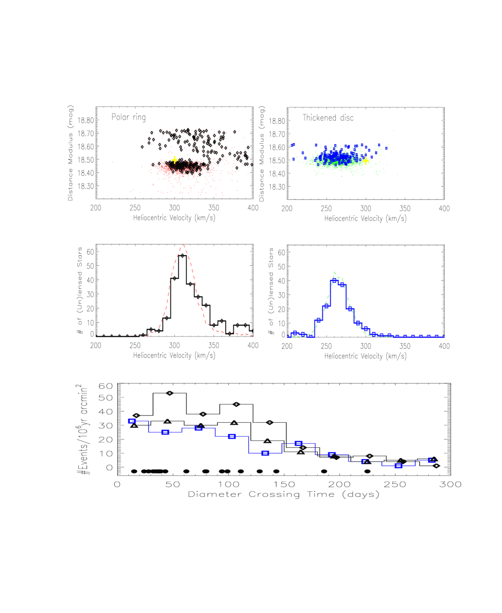
Figure 2: Upper panels: radial velocity vs. distance modulus distribution for the lensed sources in a given line of sight (diamonds for a minor axis field of the polar ring model, and squares a major axis field of the thickened disc model). Note they bias towards kinematically distinct stars behind the LMC disc, unlike unlensed random stars (small dots) in the same direction. The large crosses mark the systematic velocity and distance of the LMC. Middle panels: histograms of the radial velocity of lensed sources (solid lines with symbols) and a renormalized distribution for neighbouring unlensed stars (dashed lines). Note the wings of lensed sources. Bottom panels: histograms of predicted event time scale in bins of 1 month; the one with triangles is for a major axis field of the polar ring model. A few MACHO alerts are indicated by solid circles at the bottom.

The upper panels of Fig. 2 show the simulated velocity and distance distributions for the polar ring model in a line of sight on the minor axis of the LMC $(283^{o},-33^{o})$, and for the thickened disc model on the major axis $(280^{o},-31^{o})$. They are typical lines of sight of MACHO observed events and are chosen to have nearly the same number ($\sim 2000$) of LMC disc stars per square arcmin.

There are mainly two complementing effects shown here. First a radial velocity survey should pick up a small fraction of outliers of the rotation curve of the LMC disc, which may belong to some puffed-up distribution (be it a polar ring or a thickened disc) surrounding the LMC disc. Second the outliers at the backside of the LMC are more likely picked as lensed sources. They show up as the wings of the velocity histogram with a velocity set apart from the rotation speed of the LMC disc in the same field by typically more than $20{\mbox{\rm\,km\,s}}^{-1}$. The velocity distribution for the lensed sources has the strongest wings for the minor axis field of the polar ring model. The distribution has a probability of $10^{-17}$ (from an F-test of the variance) being the same as the distribution of the unlensed stars in the LMC. In contrast, if all events come from LMC disc stars being lensed by foreground Milky Way machos or disc stars, then the lensed sources would follow the motions of average stars in the cold, rotating disc. The confidence level here should not be taken literally given systematic uncertainties with the underlying models of the LMC.

We have run several models, varying the angle between the torus and the LMC disc. Occasionally the wings disappear even in self-lensing models, in which case the degeneracy with the macho-lensing models remains. This, for example, happens when the line of sight misses the torus-like substructure. But in general the high velocity wings appear to be generic and significant (cf. Fig. 2). The F-test gives a probability of $6\times 10^{-4}$ or $4\times 10^{-12}$ respectively for the major axis field ($+3^{o}$ from center) of the polar ring model or the thickened disc model. The above statistics are all computed for samples of a few hundred events, which is relevant for a future microlensing survey of the LMC. But even for the present, much smaller sample of $10-30$ lensing events the wings in the velocity distribution should still be at a level marginally (by about $1\sigma$) observable if self-lensing is indeed dominant.

There is one interesting variation of the polar ring model. Generally the ring is not exactly edge-on, as it has been assumed, so some LMC stars will be lensing polar ring stars at the back in one strip of the sky, and being lensed by polar ring stars in the front in another strip of the sky. Events will then be split equally between the two configurations, as it is with the thickened disc model. However, the phase-mixing of a tidal substructure will be incomplete even over a Hubble time, so a polar stream might appear only at the backside of the LMC disc. Such a polar stream or “arc” should show up as a strong signal in the velocity distribution of the lensed sources and in the sky distribution of the events.

Finally we comment briefly on the event rate and event time scale distribution (the bottom panel of Fig. 2). First note the interesting signature of self-lensing: the event duration distribution and event rate vary across the LMC because the typical lens-source relative distance and velocity all vary with line of sight. Also the long duration tails of the event distributions are generally strong because the lenses are stars with mass above the hydrogen burning limit, and the lens and the source are co-moving with relative velocity limited by the escape velocity from the LMC potential. Second, there appears to be a general shortage of stars in co-moving substructure of the LMC available as lenses or sources. The lensing rate for the polar ring model is about $0.08\times(M_{t}/2\times 10^{9}M_{\odot})f_{\rm wrap}^{-1}$ and $0.11\times(M_{t}/2\times 10^{9}M_{\odot})f_{\rm wrap}^{-1}$ per survey star per million year on the major axis and minor axis respectively, where $M_{t}$ is the mass of the 3D substructure, and the factor $f_{\rm wrap}$ takes into account that an unviralized substructure may not wrap around a full circle of the LMC, but only a fraction $f_{\rm wrap}$ of it. These event rates appear significantly (by a factor three) lower than the observed rate if we believe that the LMC disc is thin ($\leq 400$pc in FWHM), the 3-dimensional substructure (whether a polar stream or a thickened disc component) is a light ($M_{t}\leq 2\times 10^{9}M_{\odot}$) and wrapped-around symmetric component ($f_{\rm wrap}=1$), and the tidal truncation radius of both is small ($r_{t}\sim 6$kpc). To boost-up the self-lensing rate to account for all observed events, it appears necessary to (a) invoke a stubby ($f_{\rm wrap}\sim 0.1-0.5$), SMC-sized, tidal stream of the LMC lying at a few kpc either in the back or front of the LMC disc (Zhao 1998a,b), or (b) put most of the LMC’s mass in a thickened component ($M_{t}\sim 10^{10}M_{\odot}$) out to $10$kpc from the center of the LMC (Weinberg 1998). The proposed kinematic survey should place stringent limit on the fraction of older and kinematically distinct populations in the LMC disc and surrounding.

6 Strategy for the radial velocity survey

Most of current alerts and candidates of lensed source stars are about $(20\pm 1)$mag long after the microlensing event (cf. Fig. 1), and brighter than 19 mag at the peak of the amplification. They are bright enough for obtaining low resolution spectrum using 4m-8m class southern telescopes. The observations can be scheduled any time after the event. To keep up with the current turn-out rate of microlenses towards the LMC and SMC ($\leq 10$ events per year), we need about two nights each year during the latter half of the LMC/SMC season with a single/multi-slit spectrograph. As an example, we estimate that a ten-minute integration with the VLT can achieve a S/N of 10 per Å, sufficient for the radial velocity work here, for a $V=20$mag star using FORS1 in its highest resolution mode. Comparable S/N might be achieved with an one-hour exposure on other 4m class telescopes in Chile and Australia (e.g., Sahu & Sahu 1998) depending on seeing and instruments. While taking spectrum at the peak can obviously achieve the same S/N for less integration time (Lenon et al. 1996), it is probably not advisable considering its heavy demand for immediate observing.

A continuation and expansion of the MACHO survey, such as the Next Generation Microlensing Survey (NGMS, Stubbs 1998), holds the promise to raise the event turn-out rate by an order of magnitude. This involves monitoring the light curves of ten times more stars than the 9 million by the MACHO program. It effectively includes if all stars brighter than 20-21 mag. over the entire LMC. To follow up these events, a more ambitious program appears to be necessary. It is probably optimal for a 2m class telescope (such as the Du Pont 2.5m at Las Campanas) with a single-slit or multi-object capability to take spectra of every event near the peak since we expect a new source coming to maximum amplification every few nights; dedicated use during the LMC/SMC season would be most efficient. The reduced aperture is nicely compensated by the gravitational amplification; a $1.5$ magnitude amplification is roughly equivalent to doubling the aperture of the telescope. The gain of taking spectra in real time would be even greater for the rare class of high amplification events as done for MACHO-96-BULGE-3 and MACHO-98-SMC-1. The size of the source star can be inferred from the spectra, which could constrain the relative proper motion of the lens and source $|\mu_{l}-\mu_{s}|$. Very strong constraints on the lensing model can come from a combination of radial velocity and proper motion (cf. Fig. 1 of Zhao 1999a).

Another integral part of the survey is to obtain radial velocities of random stars in the LMC, particular those in the immediate neighbourhood of the lensed stars. These neighbouring stars serve both as a direct probe of the hotness of the LMC and existences of any 3D substructure and as a control sample quantifying the velocity wings of the microlensed sources. All together, the kinematic survey can be made most efficient by the following. For every microlensed source under study we can, at the same time, take spectra of $10$ (say with VLT/FORS1) to $100$ (say with AAT/2dF) well-isolated stars in the same observing field depending on the crowdness of the field and the capability of the multi-object spectrograph. The candidate list for spectra can be built from CMDs for identifying the lensed source in the first place, and only those field stars brighter than the target source star should be used for efficiency. With this strategy we expect to build a sample of $10^{3}-10^{4}$ stars in the vicinity of 10-100 lensed stars. The large sample is necessary to be sensitive to minor components; the VRC stars of Zaritsky et al. (1997, 1999) make up only a few percent of the total luminosity of the LMC. A fair sample should also include stars of a wide range of intrinsic luminosity and color so as to minimizing biasing due to different ages; the older population might be more puffed-up and rotate slower than the young, thin disc. As a by-product of the dark matter study, these kinematic samples are useful for understanding of the spatial and dynamical structure of the LMC.

7 Conclusion

Subtle systematic effects are expected for microlensed stars towards the LMC in their distributions of radial velocity, proper motion, projected distance from the center of the LMC, distance modulus and reddening (Zhao 1999a,b). While the predictions are still subject to model assumptions at different levels, detection or non-detection of these lensing-induced systematic bias in all five distributions is likely to give a robust conclusion on the nature of Galactic dark matter. The radial velocity survey is by far the most promising approach since radial velocities can be measured very accurately with access to 2m-8m southern telescopes. The survey can be done for both exotic events and common low amplification events either during lensing or at a scheduled time in the latter part of the season. Studies of the systematic bias can all be integrated in the Next Generation Microlensing Survey (Stubbs 1998) for the dark matter problem and other photometric/kinematic surveys of the LMC for the studies of structures and star formation history of the LMC (Zaritsky et al. 1999).

Table 1 shows the levels of confidence to rule out macho-lensing models (or other Type-I models with intervening material dynamically unassociated with the LMC) with the current sample and a larger sample of microlensing events in the future, assuming that we will obtain the radial velocities of all the lensed sources and unlensed stars in neighbouring lines of sight (say, within $5^{\prime}$, which is 100pc at the LMC). More than half a decade of the MACHO survey have covered more than $11$ square degrees and $9$ million stars of the LMC and SMC, and found up to 30 possible microlensing events. The total exposure is about $(0.5-1)\times 10^{8}$ in units of star year. We expect that the exposure and the number of events will be more than quadrapoled in the next few years by the on-going EROS 2 and OGLE 2 surveys, the MACHO last-year survey and some versions of NGMS. While spectra of microlensed sources have been taken sporadicly in the past (e.g. Della Valle 1994 on MACHO-LMC-1), there is a lack of differential study of kinematics and photometry with unlensed stars in the same field. As of present there is no published data on the kinematics of the microlensed sources.

Finally these differential studies of microlensing stars and unlensed stars could also be done towards the Galactic bulge where self-lensing of the Galactic bar surely plays an important role. The Space Interferometry Mission (SIM, 2005-2010) provides a more distant but exciting prospect of measuring the lensing-induced wobbling motion of the image centroid as astrometric follow-up of a few microlensing candidates from ground-based surveys.

The author thanks Wyn Evans, Ken Freeman, Puragra Guhathakurta, Rodrigo Ibata, Konrad Kuijken, Knut Olsen, Joel Primack, Penny Sackett and Chris Stubbs for helpful discussions and the anonymous referee for very helpful comments on the presentation.

Table 1: Sample size and confidence level for discriminating various microlensing hypotheses

Exposure	$N_{\rm source}$	$N_{\rm neighbour}$	Confidence	Confidence
0.5e+08	25	500	2.e-02	4.e-02
1.5e+08	75	1500	3.e-05	6.e-04
2.5e+08	125	2500	9.e-08	9.e-06
3.5e+08	175	3500	3.e-10	2.e-07
4.5e+08	225	4500	8.e-13	3.e-09
5.5e+08	275	5500	3.e-15	5.e-11

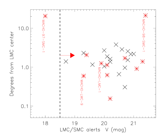
Figure 1: Magnitude and radius distribution of some 30 microlensing alerts (crosses) and published candidates (asterisks) towards the Magellanic Clouds. The dashed line marks the distance modulus of the LMC. Lensed stars should be fainter in average (direction of arrow) compared to the unlensed stars and cluster at where the LMC has the biggest line of sight depth if LMC-LMC self-lensing is important.

References

- (1) Alcock, C. et al. 1997, ApJ, 490, L59
- (2) Bothun, G.D. & Thompson, I.B. 1998, AJ, 96, 877
- (3) Della Valle, M. 1994, A&A, 287, L31
- (4) Evans, N.W. et al. 1998, ApJ, 501, L45
- (5) Freeman, K., Illingworth, G. & Oemler, A. 1983, 272, 488
- (6) Gould, A. 1994, ApJ, 421, L75
- (7) Holtzman, J. et al. 1997, AJ, 113, 656
- (8) Kroupa, P., Tout, C. & Gilmore, G. 1993, MNRAS, 262, 545
- (9) Kunkel, W. et al. 1997, ApJ, 488, L129
- (10) Lennon, D.J., Mao, S., Fuhrmann, K.& Gehren, T. 1996, ApJ 471, L23
- (11) Lu, L. et al. 1998, AJ, 115, 162
- (12) Putman, M. et al. 1998, Nature, 394, 752
- (13) Sahu, A. 1994, Nature, 370, 275
- (14) Sahu, K. C. & Sahu, M. S., 1998, ApJ, 508, L147
- (15) Stubbs, C. 1998, astro-ph/9810488
- (16) Weinberg, M. 1998, astro-ph/9811204 and astro-ph/9905305
- (17) Wu, X.P. 1994, ApJ, 435, 66
- (18) Zhao, H.S. 1998a, MNRAS, 294, 139
- (19) Zhao, H.S. 1998b, ApJ, 500, L49
- (20) Zhao, H.S. 1999a, astro-ph/9902179
- (21) Zhao, H.S.,1999b, ApJ submitted