The spectral evolution of post-AGB stars

Abstract

A parameter study of the spectral evolution of a typical post-AGB star, with particular emphasis on the evolution of the infrared colours, is presented. The models are based on the latest evolutionary tracks for hydrogen burning post-AGB stars. For such tracks the evolutionary rate is very dependent on the assumed mass loss rate as a function of time. We investigate this effect by modifying the mass loss prescription. The newly calculated evolutionary rates and density distributions are used to model the spectral evolution of a post-AGB star with the photo-ionization code cloudy, including dust in the radiative transfer. Different assumptions for the dust properties and dust formation are considered. It is shown that by varying these parameters in a reasonable way, entirely different paths are followed in the IRAS colour-colour diagram. First of all, the effects of the evolution of the central star on the expanding dust shell can not be neglected. Also the dust properties and the definition of the end of the AGB phase have an important effect. The model tracks show that objects occupying the same location in the IRAS colour-colour diagram can have a different evolutionary past, and therefore the position in the IRAS colour-colour diagram alone can not a priori give a unique determination of the evolutionary status of an object. An alternative colour-colour diagram, the K–[12] vs. [12]–[25] diagram, is presented. The tracks in this diagram seem less affected by particulars of the grain emission. This diagram may be a valuable additional tool for studying post-AGB evolution.

1 Introduction

The transition phase between the Asymptotic Giant Branch (AGB) and planetary nebulae (PNe) has gained much attention over the last decade. AGB stars lose mass fast and get obscured by their circumstellar dust. As the star leaves the AGB, its mass loss rate decreases significantly and the star may become sufficiently hot to ionize its circumstellar material and be observable as a PN. During the transition from the AGB to the PN phase (the post-AGB or proto-planetary nebula phase) the dust shell created during the AGB moves away from the central star and becomes optically thin after a few hundred years; the obscured star becomes observable. The transition time from the AGB to the PN phase is estimated to be a few thousand years (e.g. Pottasch 1984).

Whereas PN are relatively easy to find because of their rich optical emission line spectra, post-AGB stars have more inconspicuous spectra and are therefore much harder to find. The number of post-AGB stars only started to become large after the IRAS mission, that was successful in detecting objects surrounded by circumstellar dust.

Several samples of post-AGB stars are presented in the literature (e.g. Volk & Kwok 1989, Hrivnak, Kwok & Volk 1989, van der Veen, Habing & Geballe 1989, Trams et al. 1991, Oudmaijer et al. 1992, Slijkhuis 1992). Most of these objects are stars with supergiant-type spectra, surrounded by dust shells. These samples of post-AGB stars have in common that the original criteria which were employed to find them implicitly made assumptions on the spectral energy distribution (SED) of post-AGB stars. Some authors used criteria on the IRAS colours, because post-AGB stars were expected to be located in a region in the IRAS colour-colour diagram between AGB stars and PN (e.g. Volk & Kwok 1989, Hrivnak et al. 1989, van der Veen et al. 1989, Slijkhuis 1992). Other authors loosened this criterion and searched for objects in the entire colour-colour diagram, but with an additional criterion that the central star should be optically visible (e.g. Trams et al. 1991, Oudmaijer et al. 1992, Oudmaijer 1996).

Such samples are subject to selection effects, so the objects that have been selected do not have to be representative for the entire population of post-AGB stars. In order to understand these selection effects and to obtain a handle on the kinds of objects that could have been missed, it is useful to investigate the spectral energy distribution from a theoretical point of view by following the spectral evolution of a post-AGB star with an expanding circumstellar shell. Moreover, this type of study allows one to investigate and understand the processes that occur in the circumstellar shell during the transition.

Several such studies have been published. Most of these studies focus on the expanding dust shell with a dust radiative transfer model. Authors like e.g. Siebenmorgen, Zijlstra & Krügel (1994), Szczerba & Marten (1993), Loup (1991), Slijkhuis & Groenewegen (1992) and Volk & Kwok (1989) performed calculations describing the evolution of the circumstellar dust shell. Work concerning the evolution of a star with an expanding shell has also been performed with photo-ionization codes (Volk 1992), and hydrodynamical models (Frank et al. 1993, Mellema 1993, Marten & Schönberner 1991). None of these models include dust, except for Volk (1992) who used the output of the photo-ionization code cloudy (Ferland 1993) as input for a dust model.

Our objective is to investigate the spectral evolution of a hydrogen burning post-AGB star with a photo-ionization model containing a dust code. The aim of this work is twofold:
Firstly we investigate the processes in the circumstellar envelope. The emphasis in this paper will be on the infrared properties of this shell. For this, both the expansion of the shell and the evolution of the central star have to be taken into account.
Secondly, we investigate the influence of certain assumptions on the evolutionary timescales. Only few post-AGB evolutionary grids have been published, never giving a fine grid for the coolest part of the evolution. The original Schönberner tracks (1979, 1983) presented only a limited number of time points of the evolution, while Vassiliadis & Wood (1994) omit the phase between 5000 K and 10 000 K altogether. The predicted timescales that are available are calculated with a pre-defined end of the AGB and assumed post-AGB mass loss rates. These choices can influence the post-AGB evolutionary timescales considerably, as was already demonstrated by Trams et al. (1989) and Górny, Tylenda & Szczerba (1994). The situation has changed now with the results of Blöcker (1995a,b), who calculated new evolutionary sequences, and made extensive tables available describing certain key parameters during the post-AGB phase. The published relation between the envelope mass and effective temperature allows one to construct detailed timescales using one’s own mass loss prescriptions during the (post-) AGB evolution, which makes the model results less dependent on the mass loss formulation that was used by Schönberner (1979, 1981, 1983).

In this paper first we describe the method to calculate evolutionary timescales and the adopted mass loss prescriptions. The results of Blöcker (1995a,b) are used as a basis to create synthetic evolutionary tracks, and some aspects of the evolutionary timescales that are predicted are discussed. Next we describe the photo-ionization code cloudy that was used and the assumptions that were made to conduct the study of the spectral evolution of post-AGB stars. We then present the first results of a parameter study of a typical post-AGB object, based on the 0.605 M_⊙ track from Blöcker (1995b).

2 The central star evolution

Many stellar evolutionary models are presented in the recent literature, but only two groups calculate the AGB quantitatively including mass loss. These are Vassiliadis & Wood (1993, 1994) and Blöcker & Schönberner (1991) and Blöcker (1995a,b). Both groups calculate the evolution of a star from the main sequence through the red giant phase to the white dwarf stage. There are slight differences in the core mass – luminosity relations and the use of a different initial – final mass relation, but their results show qualitatively the same behaviour in the evolution of stars in the HR diagram. The main differences between the models are the mass loss prescriptions on the AGB.

The AGB mass loss rates in the formulation of Vassiliadis & Wood are derived from the mass loss – pulsation period ($\dot{M}$–$P$) relation given by Wood (1990). For periods longer than 500 d for low mass stars, and larger pulsation periods for higher mass objects, a maximum value of the AGB mass loss rate is invoked (of the order of 10^-5 M_⊙ yr^-1). Blöcker used a mass loss rate which is dependent on the luminosity of the star. He fitted the results of Bowen’s (1988) theoretical study of mass loss in Mira variables. Basically this is the Reimers mass loss (Reimers 1975) multiplied by a luminosity dependent factor. These mass loss rates are not limited by a maximum value. Since the adopted AGB mass loss rates by the above authors differ, some striking differences between the results of their calculations exist. The $\dot{M}$–$P$ relation of Wood (1990) is questioned by Groenewegen & de Jong (1994). Using the synthetic evolutionary model of Groenewegen & de Jong (1993), they were able to fit the luminosity function of carbon stars in the LMC with the Bowen mass loss adopted by Blöcker (1995a), but not with the Vassiliadis & Wood mass loss rates.

The mass loss rates do not only govern the evolution on the AGB. During the post-AGB phase, the mass loss rates also have a drastic influence on the timescales of the AGB – PN transition. Since the temperature of the star for a given core mass is determined by the mass of the stellar envelope, larger mass loss rates will cause the star to evolve to higher temperatures more quickly and can therefore decrease the timescale of the transition strongly. Trams et al. (1989) showed that when the adopted post-AGB mass loss rates of a 0.546 M_⊙ star are raised by a factor of 5 to 10 to a value of 10^-7 M_⊙ yr^-1, the transition time from the AGB to the PN phase is shortened from 100 000 yr to only 5000 yr. This would make a low mass star readily observable as a PN, while the (longer) predicted timescales prevent such objects to become an observable PN since the circumstellar shell would have moved far away from the star and would have dispersed into the interstellar medium long before the star emits a sufficient amount of ionizing photons. In order to study the evolutionary timescales of post-AGB stars, it is important to understand post-AGB mass loss better.

2.1 Determination of the evolutionary timescales

The evolutionary timescales of hydrogen burning post-AGB stars are determined by the core mass and the mass loss rates of the star. In this section we present the computational details of this procedure, compute the evolutionary timescales and investigate several aspects of these timescales. We use the tracks by Blöcker (1995a,b) to determine the evolutionary timescales. Blöcker calculated several tracks for his investigation of the evolution of stars on the AGB and beyond. The tracks include a complete calculation of a 3 M_⊙ object that ends as a 0.605 M_⊙ white dwarf and a 4 M_⊙ (0.696 M_⊙) sequence. To these sequences, the 1.0 M_⊙ (0.565 M_⊙) track of Schönberner (1983) was added. We start with a recapitulation of the mass loss laws we have used (see also Blöcker 1995b).

2.1.1 The mass loss laws

During the red giant branch, the mass loss is parameterized by the Reimers mass loss rate ${\dot{M}}_{\rm R}$ given in equation (1), where the scaling parameter $\eta$ is set to 1 for all tracks.

$${\dot{M}}_{\rm R}/({\rm{\rm M_{\odot}}\,yr^{-1}})=4\times 10^{-13}\,\eta\,\frac{(L/{{\rm L}_{\odot}})(R/{{\rm R}_{\odot}})}{(M/{\rm M_{\odot}})}$$ (1)

With $L$, $R$ and $M$ the luminosity, radius and mass of the star. Since AGB stars lose mass at a faster rate than red giants, a different formulation is adopted for the AGB mass loss rates. To this end, Blöcker fitted the numerical results of Bowen, as given in equation (2).

$${\dot{M}}_{\rm B1}/({\rm{\rm M_{\odot}}\,yr^{-1}})=$$ (2)

$\hfill 4.83\times 10^{-9}\,(M_{\rm ZAMS}/{\rm M_{\odot}})^{-2.1}(L/{{\rm L}_{\odot}})^{2.7}{\dot{M}}_{\rm R}$

$${\dot{M}}_{\rm B2}/({\rm{\rm M_{\odot}}\,yr^{-1}})=\hfill 4.83\times 10^{-9}\,(M/{\rm M_{\odot}})^{-2.1}(L/{{\rm L}_{\odot}})^{2.7}{\dot{M}}_{\rm R}$$

The difference between ${\dot{M}}_{\rm B1}$ and ${\dot{M}}_{\rm B2}$ is the division by the current mass of the star instead of the initial mass of the star. The timescales for the 0.565 M_⊙ track of Schönberner were recalculated by us using the $M_{\rm env}$–$T_{\rm eff}$ relation given by Schönberner but with the mass loss prescriptions of Blöcker. For all tracks the ${\dot{M}}_{\rm B1}$ prescription was used, except for the 0.605 M_⊙ track where ${\dot{M}}_{\rm B2}$ was used, which results in larger AGB mass loss rates.

The mass loss rates can reach values of the order of 10^-4 M_⊙ yr^-1 to 10^-3 M_⊙ yr^-1 and it is clear that if this mass loss would last for a long time, the star would evaporate. Thus, an end to the AGB (-wind) has to be invoked. Blöcker used the pulsation period to define the end of the high mass loss phase; he assumed that AGB stars pulsate in the fundamental mode, where the period can be calculated using equation (3) (Ostlie & Cox 1986).

$$\lg(P_{0}/{\rm d})=-1.92-0.73\lg(M/{\rm M_{\odot}})+1.86\lg(R/{{\rm R}_{\odot}})$$ (3)

When the central star has reached an inferred pulsation period of $P_{\rm a}$ = 100 d (which occurs when the star has a surface temperature somewhere between roughly 4500 K and 6000 K) the Bowen mass loss stops. When the star has subsequently reached an inferred pulsation period of $P_{\rm b}$ = 50 d the post-AGB mass loss starts; in between the mass loss rates are connected by a smooth transition. Hence the following definitions will be used in the remainder of the paper: the AGB phase is that part of the evolution where the pulsation period is greater than $P_{\rm b}$, the (AGB) transition phase is that part of the evolution where the pulsation period is in between $P_{\rm a}$ and $P_{\rm b}$, and finally the post-AGB phase is that part of the evolution where the pulsation period is smaller than $P_{\rm b}$.

One should realize that post-AGB stars with pulsation periods larger than 50 d exist (e.g. HD 52961 with a period of 72 d; Waelkens et al. 1991, Fernie 1995). Thus the pulsation period recipe used by Blöcker should only be regarded as an approximate parameterization of the end of the AGB.

For lower temperatures the post-AGB mass loss is given by the Reimers law (1). Since the Reimers mass loss is proportional to $T_{\rm eff}$^-2 for a constant luminosity and stellar mass, the post-AGB mass loss rates decrease during the evolution of the object. A radiation driven wind will take over when the star has reached temperatures above approximately 20 000 K. The mass loss rate for this wind, based on Pauldrach et al. (1988), is given by equation (4). Hence at any stage of the post-AGB evolution either equation (1) or (4) is used, whichever of the two yields the biggest mass loss.

$${\dot{M}}_{\rm CPN}/({\rm{\rm M_{\odot}}\,yr^{-1}})=1.29\times 10^{-15}\,(L/{{\rm L}_{\odot}})^{1.86}$$ (4)

During the evolution on the AGB and beyond, the envelope mass is reduced due to two processes. In the outer parts of the envelope, mass is lost through a wind, and at the bottom of the envelope, mass is diminished by hydrogen burning. From Trams et al. (1989) we find the mass loss due to hydrogen burning:

$${\dot{M}}_{\rm H}/({\rm{\rm M_{\odot}}\,yr^{-1}})=1.012\times 10^{-11}\,(L/{{\rm L}_{\odot}})X_{\rm e}^{-1}$$ (5)

With $X_{\rm e}$ the hydrogen mass fraction in the envelope (70 %).

2.1.2 The evolutionary timescales

The evolutionary timescales for hydrogen burning post-AGB stars depend firstly on the core mass and secondly on the mass loss rates. The evolutionary timescales can be calculated relatively easy by making use of the fact that there exists a unique relation between the envelope mass and the stellar temperature for every core mass. One can calculate the evolutionary timescales by combining this relation with the mass loss prescriptions given in the previous section. Dr. Blöcker kindly provided us with tables from which the $M_{\rm env}$–$T_{\rm eff}$ relation could be reproduced.

The timescale for the envelope depletion is given by:

$$\frac{\Delta M_{\rm env}}{\Delta t}={\dot{M}}_{\rm wind}+{\dot{M}}_{\rm H}$$ (6)

Using the $M_{\rm env}$–$T_{\rm eff}$ relation this expression can be transformed into an expression for the evolutionary rate $\Delta T_{\rm eff}/\Delta t$ of the central star

$$\frac{\Delta T_{\rm eff}}{\Delta t}=\frac{\Delta T_{\rm eff}}{\Delta M_{\rm env}}\times\frac{\Delta M_{\rm env}}{\Delta t}=\frac{{\dot{M}}_{\rm wind}+{\dot{M}}_{\rm H}}{\frac{\mbox{\rm d}M_{\rm env}}{\mbox{\rm d}T_{\rm eff}}}$$ (7)

Integrating this expression yields the actual timescales for the evolution of the central star.

In Fig. 1 some relations are presented for the 0.565 M_⊙, 0.605 M_⊙ and 0.696 M_⊙ tracks. The upper panel shows the envelope mass as function of photospheric temperature. The second panel presents the mass loss rates as function of temperature, and the third panel shows the evolutionary rate in kelvin per year as function of temperature. In the second panel it is visible that the transition phase occurs at higher temperatures for larger core masses with the recipes described above.

Figure 1: The $M_{\rm env}$–$T_{\rm eff}$ relations, mass loss rates and resulting evolutionary rates for the 0.565 M_⊙ (dotted line), 0.605 M_⊙ (solid line) and 0.696 M_⊙ (dashed line) tracks. The envelope mass is given in solar masses, the mass loss rate in solar masses per year and the evolutionary rate in kelvin per year. Note that the 0.605 M_⊙ track has a larger AGB mass loss rate. For this particular track, the B2 mass loss rate was used.

The evolutionary rate, mass loss rate and envelope mass are related to each other in the following way. The evolutionary rate in terms of increase in temperature per year is slow on the steep part of the $M_{\rm env}$–$T_{\rm eff}$ relation, and more rapid on the shallow part. Larger mass loss rates imply of course more rapid changes in the stellar temperature. These effects are visible in Fig. 1: at low temperatures in the post-AGB phase the evolutionary rates are smallest, while for higher temperatures the evolutionary rate increases. The minima around lg($T_{\rm eff}$/K) $\approx$ 3.7 to 3.9 correspond to the onset of the smaller post-AGB mass loss, slowing down the evolution which accelerates later on the shallow part of the $M_{\rm env}$–$T_{\rm eff}$ relation.

Interestingly, the minimum in the evolutionary rate occurs right after the end of the AGB transition phase. The net increase in effective temperature in kelvin per year is the slowest for all tracks just after the start of the post-AGB evolution, which is when the temperature of the objects correspond to G or F spectral types. The increase in temperature is less than 1 K yr^-1 for the 0.565 M_⊙ and 0.605 M_⊙ tracks. How does this evolutionary rate compare with the observations? Fernie & Sasselov (1989) calculated the possible increase in temperature for UU Her stars. From the absence of a change in pulsation period of UU Her, 89 Her and HD 161796, they place an upper limit of 0.5 K yr^-1 on the temperature increase. Their conclusion was that these objects can not be post-AGB stars because the evolutionary rates should be much higher. However, this may be the case when one averages over the entire post-AGB temperature span, but the observed lack of temperature increase is consistent with the predictions for this temperature range, as was already shown by Schönberner & Blöcker (1993). Therefore a post-AGB nature for the UU Her stars can not be excluded on this basis.

2.2 The influence of mass loss on the evolutionary timescales

It is evident from the above that the value of the post-AGB mass loss rate has an important effect on the evolutionary timescales. However, the mass loss rate is not known observationally for cool post-AGB stars. The usual tracer of mass loss, H$\alpha$ emission, which is often observed in the spectra of post-AGB objects is likely to be the result of stellar pulsations (see the discussion by Oudmaijer & Bakker 1994 and Lèbre et al. 1996). A possible tracer of mass loss in cool post-AGB stars is the CO first-overtone emission at 2.3 $\mu$m (Oudmaijer et al. 1995), but, given this is true, the mass loss rates still have to be determined.

The lack of theoretical and observational values for post-AGB mass loss rates forced Schönberner and Blöcker to resort to the heuristic Reimers law for the cool part of the post-AGB evolution. As an illustration of the effect of the post-AGB mass loss rates on the evolutionary timescales, we have calculated these timescales for three core masses with the post-AGB mass loss rate at 0, 1, 5 and 10 times the standard post-AGB value (indicated as 0$\times$pAGB etc.). The results for the 0.565 M_⊙, 0.605 M_⊙ and 0.696 M_⊙ tracks are presented in Table 1, where the timescales since the end of the transition mass loss phase are given. The increase of the post-AGB mass loss rates indeed decreases the timescales of the evolution, confirming the results of Trams et al. (1989) and Górny et al. (1994). The 0$\times$pAGB mass loss rate effectively determines the slowest possible evolutionary speed, since the only mass loss is through hydrogen burning. On average, the difference in speed between 0$\times$pAGB and 1$\times$pAGB is roughly a factor of two to three.

Table 1: Evolutionary timescales for different values of post-AGB mass loss rates; the post-AGB phase starts at $P_{\rm b}$ = 50 d.

${\dot{M}}_{\rm PAGB}$	0$\times$pAGB	1$\times$pAGB	5$\times$pAGB	10$\times$pAGB
$T_{\rm eff}$ (K)
$M_{\rm core}$ = 0.565 M⊙, $L$ = 3891 L⊙
5 426	0	0	0	0
5 500	312	76	18	9
6 000	1113	286	70	36
7 000	2810	815	207	107
10 000	3974	1306	349	182
15 000	5172	2092	651	353
20 000	6383	3089	1141	653
25 000	7544	4156	1768	1068
30 000	8709	5292	2526	1604
$M_{\rm core}$ = 0.605 M⊙, $L$ = 6310 L⊙
6 042	0	0	0	0
6 500	1671	458	113	58
7 000	2510	715	178	92
10 000	3122	948	241	125
15 000	3487	1181	325	171
20 000	3822	1458	452	248
25 000	4154	1769	625	358
30 000	4481	2093	832	501
$M_{\rm core}$ = 0.696 M⊙, $L$ = 11 610 L⊙
6 846	0	0	0	0
7 000	94	29	7	4
7 500	192	62	15	8
10 000	245	84	22	11
15 000	287	111	30	16
20 000	309	129	38	21
25 000	331	151	50	28
30 000	354	174	65	38

2.3 Distribution over spectral type

The availability of the evolutionary rates allows us to investigate the predicted distribution over spectral type. Oudmaijer, Waters & Pottasch (1993) and Oudmaijer (1996) used the coarse grid of the Schönberner (1979, 1983) tracks and found that a star spends by far most of the time as a B-type star. Only for the 0.644 M_⊙ track half of the time is spent in the G phase, and somewhat less as a B star, while almost no time is spent as an F or A star.

One might not expect that an object would spend a large fraction of the time as a B star, because the evolutionary rates are largest for B spectral type (Fig. 1). This can be understood however when we consider the large range of temperatures that corresponds to spectral type B: roughly between 10 000 K and 30 000 K. In contrast, A stars only have a temperature range between approximately 7500 K and 10 000 K. The large evolutionary rates multiplied by the temperature range then result in a longer time spent as a B star during the post-AGB evolution. The large fraction of time that is spent as a G star in the 0.644 M_⊙ track is explained by the steep $M_{\rm env}$–$T_{\rm eff}$ relation for temperatures less than approximately 6000 K, as can be deduced from equation (7). The distribution over spectral type for the tracks presented here with 1$\times$pAGB mass loss is calculated using the conversion from effective temperature to spectral type listed by Straižys & Kuriliene (1981). These are $T_{\rm eff}$(A0I) = 9800 K, $T_{\rm eff}$(F0I) = 7400 K and $T_{\rm eff}$(G0I) = 5700 K.

To allow for a comparison with the distributions presented by Oudmaijer et al. (1993) we will assume in this section that the post-AGB phase starts when $T_{\rm eff}$ = 5000 K and ends when $T_{\rm eff}$ = 25 000 K. The distributions can be easily obtained by calculating the time spent as a G star (5000 K – G0), F star (G0 – F0) etc., and subsequently dividing these numbers by the total time spent as a post-AGB star. The resulting distributions are plotted in Fig. 2. For comparison the distribution over spectral type of the sample of 21 post-AGB objects in the list of Oudmaijer et al. (1992) is given. The observed distribution peaks at F, while no B stars are found at all.

One should realize that planetary nebula central stars with temperatures below 25 000 K are observed: e.g. IRAS19336–0400 with $T_{\rm eff}$ = 23 000 K (Van de Steene, Jacoby & Pottasch 1996, Van de Steene & van Hoof 1995). Hence one could also assume an upper limit of 20 000 K for the post-AGB regime. However, the distribution over spectral type is not very different in this case, the fraction of B-type stars will be lower by approximately 10 %.

Figure 2: Distribution over spectral type. Upper left panel; the post-AGB candidate stars in the sample of Oudmaijer et al. (1992), the other panels show the predicted distribution for the 0.565 M_⊙, 0.605 M_⊙ and 0.696 M_⊙ tracks.

The 0.605 M_⊙ distribution is different from the results presented by Oudmaijer et al. (1993) for the 0.598 M_⊙ Schönberner track. In the present plot, the distribution peaks at F, while the 0.598 M_⊙ distribution peaks at G. The distribution for the same track is different in Oudmaijer (1996), since there the evolutionary timescales were shortened by 1000 yr ‘in order to make the old 0.598 M_⊙ track consistent with the new calculations’ (Marten & Schönberner 1991). This resulted in a distribution that strongly peaks at spectral type B.

The main differences between the old 0.598 M_⊙  and new 0.605 M_⊙ calculations are the progenitor mass of the star (1 M_⊙ and 3 M_⊙ respectively), the mass loss prescriptions and the definition of the end of the AGB. In the Schönberner calculations, no transition wind was assumed: the AGB mass loss would abruptly change into a post-AGB wind at 5000 K. In the Blöcker calculations, a transition wind is assumed between 5000 K and 6000 K for the 0.605 M_⊙ track. This implies shorter timescales for the G type phase of the 0.605 M_⊙ track with respect to the older calculations, but does not affect the time spent as F, A or B stars, where for both tracks a Reimers post-AGB mass loss is assumed. The only explanation we can find for the apparent difference in evolutionary speed is that the dependence of the temperature on the envelope mass of the 0.605 M_⊙ track is different from the 0.598 M_⊙ track. Apparently, the slope of the $M_{\rm env}$–$T_{\rm eff}$ relation can differ significantly for stars with a different evolutionary past, even when the resulting core masses are nearly identical.

The predicted distributions in Fig. 2 show large differences. For the smallest core mass, most of the time is spent as a B star. For the 0.605 M_⊙ case the lifetime is distributed evenly over the F and B phase. The fastest track with a core mass of 0.696 M_⊙ shows a minimum at A, while the rest of the lifetime is spread evenly over G, F and B. The 0.605 M_⊙ distribution nicely reproduces the observed peak at F. However, all tracks predict many more B stars than observed.

In order to compare the observed and predicted distributions more quantitatively, we have performed a Kolmogorov-Smirnov test using both an upper limit of 20 000 K and 25 000 K for the post-AGB regime. The resulting probabilities are given in Table 2. From these tests it appears that 0.565 M_⊙ track is an unlikely model for the observed post-AGB sample. On the other hand, the 0.605 M_⊙ and the 0.696 M_⊙ tracks can not be excluded. Given the fact that stars on the 0.696 M_⊙ track evolve much faster than on the 0.605 M_⊙ track, they would constitute only a small fraction of the total number of observable post-AGB stars. We will adopt the 0.605 M_⊙ track to describe the post-AGB evolution in the remainder of this paper.

Table 2: The results of the Kolmogorov-Smirnov test comparing various evolutionary tracks with the observed post-AGB sample. The tests have been performed using a range of temperatures for the post-AGB regime of 5000 K to 20 000 K (second column) or alternatively 5000 K to 25 000 K (third column).

track	probability	probability
M⊙	20 000 K	25 000 K
0.565	4.5$\times 10^{-4}$	2.8$\times 10^{-6}$
0.605	2.4$\times 10^{-2}$	6.4$\times 10^{-4}$
0.696	6.7$\times 10^{-2}$	1.3$\times 10^{-1}$

This exercise shows that the predictions of the distribution over spectral type are subject to large uncertainties, depending both on the $M_{\rm env}$–$T_{\rm eff}$ relation and the assumed mass loss prescription. However, regardless what assumptions are made, one would expect a fair number of B-type post-AGB stars, which are not observed in the sample depicted in Fig. 2. Hence this discrepancy remains unresolved. Reversely it can be stated that when a larger sample of post-AGB stars with reliable temperature determinations becomes available, the procedure described here can be a very effective means for testing evolutionary tracks.

3 The model

In order to calculate the spectral evolution of post-AGB stars, we used the photo-ionization code cloudy version 84.12a (Ferland 1993). Some modifications have been made to the code to facilitate the computations. The most important change was the introduction of several broadband photometric filters, including the Johnson and the IRAS filters. The in-band fluxes for these filters were calculated by folding both the spectral energy distribution and the emission line contribution with the filter passband. Internal extinction due to continuum opacities was included both in the continuum and the line contribution.

A dust model written by P.G. Martin was already included in the original code. For our modeling we used the grain species labelled ‘ISM Silicate’ and ‘ISM Graphite’. The optical constants were taken from Martin & Rouleau (1991). The absorption and scattering cross sections were calculated assuming a standard ISM grain size distribution (Mathis, Rumpl & Nordsieck 1977). All calculations were done assuming a dust-to-gas mass ratio of 1/150. For the chemical composition of the gas we assumed the abundances given in Aller & Czyzak (1983), supplemented with educated guesses for elements not listed therein (as given in cloudy).

The original code only allowed for the computation of a model with a constant dust-to-gas ratio throughout the entire nebula. However, the density profiles we calculate extend from the stellar surface outward. It is not realistic to assume that dust is present near the stellar surface and therefore we introduced new code in cloudy to solve this problem. This enabled the dust to exist only outside a prescribed radius or, alternatively, only in those regions where the equilibrium temperature of the dust would be below a prescribed sublimation temperature. These prescriptions work as a binary switch: at a certain radius either no dust or the full amount is present. In those regions where dust exists, the dust-to-gas ratio is assumed to be constant.

Two models for the dust formation are adopted. In the first model it is assumed that dust is only formed in the AGB wind, hence in material that was ejected before the stellar pulsation period reached $P_{\rm b}$. We will call this the AGB-only dust formation model. In the second model it is assumed that the dust formation continues in the post-AGB wind. We will call this the post-AGB dust formation model. Due to limitations of the code, which we discuss below, we will only investigate the spectral evolution after the post-AGB phase has started. This implies that for the AGB-only dust formation model, the inner dust radius is already at a distance from the central star and the equilibrium temperature of the grains is always below the sublimation temperature. In the post-AGB dust formation model we assume that dust only exists in those parts of the nebula where the equilibrium temperature of the grains is below the sublimation temperature. The assumed values for the sublimation temperature are 1500 K for graphite and 1000 K for silicates.

It should be noted that we only try to model dust formation and not the destruction of grains by the stellar UV field or shocks. Especially in the AGB-only dust formation model the grains at the inner dust radius are always exposed and it is expected that they eventually will be destroyed. However, little is known about grain destruction, and the rates at which this destruction occurs are very uncertain. In the case of continuing dust formation in the post-AGB wind this problem can be expected to be of lesser importance since there is a constant supply of new grains shielding the older grains.

The radiative transport in cloudy is treated in one dimension only, i.e. the equations are solved radially outwards. This assumption makes the code unsuitable to compute models of nebulae with significant amounts of scattered light and/or diffuse emission when the nebula has a moderate to high absorption optical depth. For low optical depths re-absorption of diffuse emission in the nebula is negligible and the assumptions in cloudy work very well. However, for moderate to high optical depths the re-absorption of diffuse emission that is produced in the outer parts of the nebula and is radiated inwards becomes important. The assumptions made in cloudy make it impossible to account for this energy source, nor for the amount of flux absorbed in these regions. Since the circumstellar envelope is optically thick in the AGB phase, our calculations always start shortly after the transition from the AGB to the post-AGB phase is complete.

For low temperature models the only source of diffuse light at optical and UV wavelengths is scattering of central star light by dust grains; for the highest temperature models bound-free emission also plays a role. Since for the highest temperatures the models have a low absorption optical depth, the bound-free emission causes only minor problems and we can judge the quality of the models primarily by investigating the (wavelength-averaged) scattering optical depth. An example of this approach will be shown in Section 4.

In the calculations, the central star was assumed to emit as a blackbody. All the models were calculated for a distance of 1 kpc.

3.1 Density profiles of the circumstellar shell

The density profiles of the expanding shell are calculated for the homogeneous and spherical case. Using the mass loss prescriptions described above and assuming an outflow velocity they can be calculated for any moment in time $t$.

$$\rho(r,t)=\frac{{\dot{M}}_{\rm wind}(t_{\rm ej})}{4\pi r^{2}(t,t_{\rm ej})v_{\rm exp}(t_{\rm ej})}$$ (8)

with

$$r(t,t_{\rm ej})=R_{\ast}(t_{\rm ej})+(t-t_{\rm ej})v_{\rm exp}(t_{\rm ej})$$

the distance from the centre of the star, $R_{\ast}$ the stellar radius; $t_{\rm ej}$ stands for the time when a certain layer was ejected, $v_{\rm exp}$ is the expansion velocity of the wind at the moment of ejection. It is assumed to be constant thereafter and hydrodynamical effects are neglected (see also Section 3.3). In particular, the post-AGB wind has a higher velocity than the AGB shell and will eventually overtake it. That part of the post-AGB wind which has done so contains little mass and is simply discarded.

3.2 The AGB circumstellar shell

The AGB shell is the principal contributor to the IRAS fluxes, and it is necessary to have a good description of the stellar temperature as function of the time during the AGB, in order to compute the mass loss history using equation (2). The $M_{\rm env}$–$T_{\rm eff}$ relation discussed in Section 2.1.2 starts at temperatures roughly between 3000 K and 4000 K (the relations we received from Blöcker extend to lower temperatures than given in his paper). A description of the AGB evolution for lower temperatures is lacking. Unfortunately, the evolution of $T_{\rm eff}$ and $L$ on the AGB is not shown in the Blöcker papers. We therefore simply extrapolate the $M_{\rm env}$–$T_{\rm eff}$ relation logarithmically to lower temperatures. The ‘AGB’ star then evolves according to the extended relation. The $M_{\rm env}$–$T_{\rm eff}$ relation rises rather steeply at the low temperature end so that only a limited amount of extrapolation is necessary. In this way we find reasonable start temperatures for the AGB. Since our method implicitly assumes that the luminosity remains constant during the AGB, the Bowen mass loss rates decrease with temperature. We investigate two different cases of AGB mass loss in the extrapolated part of the $M_{\rm env}$–$T_{\rm eff}$ relation: the normal Bowen mass loss and a constant mass loss held at the value of the Bowen mass loss rate at the first point of the $M_{\rm env}$–$T_{\rm eff}$ relation as given by Blöcker. These choices do not have implications for the post-AGB evolution.

3.3 Expansion velocities

The observed mean expansion velocity of AGB winds is 15 km s^-1 (Olofsson 1993), and this will be used as the typical AGB outflow velocity. During the post-AGB phase the situation is different. Slijkhuis & Groenewegen (1992) assumed that the post-AGB wind has the same outflow velocity (15 km s^-1) as the AGB wind. The escape velocity (and hence also the outflow velocity) increases with temperature however. The increasing radiation pressure from the hotter star on the less dense post-AGB wind accelerates the dust and will decrease the densities in the post-AGB wind. The escape velocity for a 10 000 K star is already of the order of 100 km s^-1 to 150 km s^-1. In addition, Szczerba & Marten (1993) found that dust was accelerated to 150 km s^-1 during the post-AGB phase. We therefore assume an expansion velocity of 150 km s^-1 in the post-AGB phase.

One should realize that the scenario of a fast wind that follows a slow wind results in a collision between the two winds (as shown by e.g. Mellema 1993 and Frank et al. 1993). When inspecting the plots of Mellema (1993) we find that the effects of the colliding winds only start to become significant when the radiation driven wind (${\dot{M}}_{\rm CPN}$) with velocities in excess of thousands of kilometers per second has developed. The effect of colliding winds will be neglected in the further calculations in this paper.

4 The model runs

Table 3: The calculated runs for the 0.605 M_⊙ track, with an initial envelope mass of 2 M_⊙, and an AGB expansion velocity of 15 km s^-1.

Run	$v_{\rm PAGB}$	$P_{\rm a}$	$P_{\rm b}$	Constant
	(km s-1)	(d)	(d)	mass loss
1	15	100	50	yesno
2	15	100	50	yes
3	150	100	50	yes
4	150	100	50	yesno
5	150	125	75	yesno
6	1500	100	50	yesno
7	150	125	75	yes

In this section we will investigate the spectral evolution of a post-AGB star by varying certain parameters that influence the mass loss rate, wind velocity and the evolutionary speed of the central star. We restrict ourselves to the 0.605 M_⊙ track and the emphasis will be on the infrared properties of the dust shell around the star. We calculated a total of seven runs. Every individual run consists of four different series of models. These individual models represent post-AGB shells with carbon-rich or oxygen-rich dust, both with and without dust formation in the post-AGB wind. We assumed the total mass of the AGB and post-AGB shell to be 2 M_⊙. With the extrapolated $M_{\rm env}$–$T_{\rm eff}$ relation this implies a start temperature of the AGB of 2543 K. The different run parameters are outlined in Table 3.

The main differences between the runs are threefold. Firstly, as stated above, the post-AGB wind velocity is subject to uncertainty. In order to assess the influence of this velocity we used three different values: 15 km s^-1, 150 km s^-1 and 1500 km s^-1. Secondly, the differences between a decreasing AGB mass loss rate and a constant mass loss rate are investigated. In the second case the constant mass loss is kept at the value of the Bowen mass loss rate at the first point of the $M_{\rm env}$–$T_{\rm eff}$ relation as given by Blöcker. This value for the mass loss of $\dot{M}$= 1.99$\times 10^{-4}$ M_⊙ yr^-1 will then be adopted throughout the extrapolated part of the $M_{\rm env}$–$T_{\rm eff}$ relation, i.e. for temperatures between 2543 K and 3743 K. Approximately 85 % of the total shell mass is ejected in this phase. Thirdly, the definition of the end of the AGB is adjusted. As an alternative the pulsation periods that define the start of the transition wind and the start of the post-AGB phase are set to 125 d and 75 d respectively, which corresponds to a transition phase occurring between 4723 K and 5418 K. For these runs the start of the transition period (defined by $P_{\rm a}$) will be reached earlier, however the transition period itself will take much longer due to the fact that the $M_{\rm env}$–$T_{\rm eff}$ relation is much steeper now in the transition region, making the evolutionary speed much slower. This gives the paradoxical result that an earlier start of the transition phase gives rise to a later start of the post-AGB phase. Also the smaller mass loss rates result in a slower evolution between 5418 K to 6042 K (the start of the post-AGB phase in the ($P_{\rm a}$,$P_{\rm b}$) = (100d,50d) runs). After the star has reached $T_{\rm eff}$ = 6042 K, the post-AGB mass loss rates are the same, and consequently the evolutionary speed in terms of kelvin per year is identical.

The models are calculated at the temperatures listed in Table 4. The second and third entries in this table reflect the time that has passed since the end of the transition wind for the ($P_{\rm a}$,$P_{\rm b}$) = (100d,50d) and ($P_{\rm a}$,$P_{\rm b}$) = (125d,75d) case respectively.

Table 4: The ages of the different models since the end of the AGB transition phase. The age of the AGB shell, in the case of the ($P_{\rm a}$,$P_{\rm b}$) = (100d,50d) models (= normal end), is 6465 yr in the case of a decreasing mass loss and 10 326 yr in the case of a constant mass loss. For the ($P_{\rm a}$,$P_{\rm b}$) = (125d,75d) models (=early end), these ages are 6741 yr and 10 603 yr respectively.

^† These models are not shown in the graphite tracks in Figs. 3 and 7.

^‡ These models are not shown in the tracks in Fig. 10.

$T_{\rm eff}$	t(normal)	t(early)		$T_{\rm eff}$	t(normal)	t(early)
(K)	(yr)	(yr)		(K)	(yr)	(yr)
5 450		553		9 000	904†	5510
5 500		1308		9 500	926†	5532
5 550		1950		10 000	948	5553
5 600		2492		11 000	991†	5597
5 700		3328		12 000	1036	5642
5 800		3904		13 000	1082†	5688
6 000		4528		14 000	1131	5736
6 050	13	4619‡		15 000	1180†	5786
6 100	89	4695‡		16 000	1232	5838
6 150	154	4760‡		17 000	1286†	5892
6 200	211	4817‡		18 000	1342	5947
6 250	262	4867		19 000	1399†	6004
6 500	457	5063		20 000	1457	6063
7 000	715	5320		25 000	1768	6374
7 500	823	5429		30 000	2093†	6699
8 000	860	5466		35 000	2409	7014
8 500	883†	5488

We will start with the results of run 4, which we will use as a reference since we consider the parameters for this run the most realistic. Subsequently we discuss the main differences between this model run and the other runs. The main results of run 4 are visualized in Fig. 3, where the tracks in the IRAS colour-colour diagram are plotted, in Fig. 4 where certain fluxes are plotted, and in Figs. 5 and 6 where a selection of spectral energy distributions is presented. In these figures a distance of 1 kpc to the object is assumed. We will discuss the results for the oxygen-rich and carbon-rich dust separately.

For this run we have made an estimate for the wavelength-averaged scattering optical depth (see also the discussion in Section 3). For the models without post-AGB dust formation the results are shown in Fig. 4. The results for the models with post-AGB dust formation are not shown, but they are almost identical. It can be seen that the scattering optical depth for the silicate and graphite models are very similar, while on the other hand the absorption optical depth is much higher for the graphite models when compared to the silicate models (this can be judged by comparing the V magnitudes for both models). This is caused by a combination of two effects. Firstly, graphite is a very efficient absorber at optical wavelengths and a relatively less efficient scatterer. The reverse is the case for silicates. This tends to level out the differences. Secondly, in the averaging process the optical depths are weighted by the output spectrum. This spectrum peaks much more towards the red for the graphite models due to the higher internal extinction. The scattering optical depth is lower at longer wavelengths and this tends to level out the differences even further. The latter effect also explains why the scattering optical depth drops off so slowly, or even rises towards higher temperatures. The peak of the energy distribution shifts towards the blue, where the scattering efficiency is much higher, thus countering the effects of the dilution of the circumstellar envelope.

Using these results we were able to obtain a worst case estimate for the amount of energy that could have been missed in the dust emission due to the fact that the scattering processes were not properly treated in our models. The amounts for the models shown in Fig. 4 are typically 10 % to 20 % of the total far-IR flux for the silicate models, and 5 % to 10 % for the graphite models. The worst case estimates for the models not shown in Fig. 4 are all below 40 %. These estimates reflect on the accuracy of the absolute fluxes and magnitudes predicted by our models. However, they are expected to cancel in a first order approximation when colours are calculated. Therefore we decided to omit the lowest temperature models whenever absolute fluxes are shown, but to include them when colours are shown.

Scattering processes will not only influence the total amount of energy absorbed, but also the run of the dust temperature with radius. This can influence the shape of the spectrum and hence also the colours. It is impossible to make an estimate for the magnitude of this effect and we will assume it to be negligible.

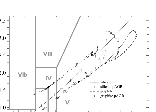
Figure 3: IRAS colour-colour diagram – run 4. The arrows indicate the evolution of the IRAS colour with time. The definitions for the IRAS colours are as presented in Oudmaijer et al. (1992). With these definitions the Rayleigh-Jeans point, where objects hotter than approximately 2000 K are found, is located at (0,0). The boxes as defined by van der Veen & Habing (1988) are drawn in. The straight line represents the blackbody line. Selected temperatures are indicated. The first data point for all tracks is the $T_{\rm eff}$ = 6050 K model.

Figure 4: The V magnitude and the 12 $\mu$m, 25 $\mu$m and 60 $\mu$m flux densities as function of temperature during the post-AGB evolution for the 0.605 M_⊙ run 4 models. The solid lines represent the models without dust formation in the post-AGB outflow. The dashed lines indicate the models with dust formation in the post-AGB wind. In the panels where no dashed lines are visible, the values are indistinguishable. All curves start at $T_{\rm eff}$ = 6100 K, except the curves for graphite with post-AGB dust formation which start at 6200 K.

4.1 Silicate dust

We will start with a description of the silicate tracks in the IRAS colour-colour diagram (Fig. 3). At first the [12]–[25] and [25]–[60] colours both increase. At some point the [25]–[60] colour remains constant, while [12]–[25] still increases. This is followed by a decrease in both the [12]–[25] and [25]–[60] colours. Hence the track makes a clockwise loop in the colour-colour diagram.

The first part of the track represents the cooling of the dust shell due to its expansion. From Table 4 one sees the inner radius of the shell has increased by a factor of 4 between $T_{\rm eff}$ = 6200 K and $T_{\rm eff}$ = 8000 K, which leads to a cooling and a decrease of the IRAS fluxes (Fig. 4). The following evolution in the IRAS colour-colour diagram is rather counter-intuitive. Normally one would expect that the shell would make the familiar counter-clockwise loop in the colour-colour diagram as found by Loup (1991), Volk & Kwok (1989) and Slijkhuis & Groenewegen (1992). In such a loop, the shell continues to cool, until the photospheric radiation begins to dominate the emission, first at the 12 $\mu$m band. At this time, the 25 $\mu$m flux and the [12]–[25] colour decrease strongly due to the expansion and cooling of the shell. The [25]–[60] colour will continue to increase slowly. Later, as the star starts to dominate at 25 $\mu$m, the [12]–[25] colour will remain constant and the [25]–[60] colour will start to decrease. When the star is the dominant contributor in all three IRAS bands, the loop will end in the Rayleigh-Jeans point. However, the above authors assumed a constant temperature of the central star, while the effects of an evolving star on the IRAS colours can not be neglected; in the 0.605 M_⊙ track the star rapidly evolves toward higher effective temperatures. For example, the kinematic age of the shell, and thus its outer (or inner) radius, has increased by only 25 % between $T_{\rm eff}$ = 8000 K and $T_{\rm eff}$ = 12 000 K. One can regard the circumstellar shell as essentially stationary around the evolving star. An evolving star embedded in a stationary shell results in a heating of the dust and an increase of the IRAS fluxes (Fig. 4). The effect of re-heating of the circumstellar envelope was already found by Marten, Szczerba & Blöcker (1993) in their calculations. The re-heating continues even beyond the last data point, hence in the colour-colour diagram the track keeps evolving to higher colour temperatures in both colours. Around the turning point the 12 $\mu$m flux is partly due to the photosphere. The photospheric flux decreases for higher temperatures so that the 12 $\mu$m flux reacts later to the rising dust flux than the 25 $\mu$m and 60 $\mu$m flux. Therefore the [12]–[25] colour starts decreasing later than the [25]–[60] colour. The result is a clockwise loop in the colour-colour diagram.

Figure 5: The spectral energy distribution at several stages during the post-AGB evolution. The upper panel shows the SED for silicate dust without post-AGB dust formation, the lower panel with dust formation, both for run 4. The flux densities are calibrated for an assumed distance of 1 kpc. The temperatures are indicated. Note the presence of the silicate emission feature at 10 $\mu$m in the post-AGB dust models.

Figure 6: As the previous figure, but now for graphite with and without post-AGB dust formation (lower panel, respectively upper panel). Note the hot dust that emits strongly in the near-infrared, but hardly contributes to the 12 $\mu$m flux density.

One should note the behaviour of the IRAS flux densities in Fig. 4. The flux densities reach a minimum during the slow evolution of the star. The minimum is followed by gradual increase in the total infrared output due to the heating of the shell resulting from the increasing absorbing efficiency of the dust (see also the discussion in Section 4.2). A model star like this (i.e. with silicate dust) would have a larger chance of being detected in an infrared survey like IRAS when it has evolved to higher temperatures. This fact, combined with the predicted distribution over spectral type implies that hot post-AGB stars, or young PN should be expected to be more abundant in samples of evolved stars with infrared excess.

4.1.1 Dust formation in the post-AGB wind

The addition of dust formation in the post-AGB wind changes the spectral energy distribution. From Fig. 4 it is visible that the 25 $\mu$m and 60 $\mu$m flux densities have the same values as in the AGB-only dust formation case. The 12 $\mu$m band is strongly affected by the addition of the hot dust. This is due to the presence of the 10 $\mu$m silicate emission feature which causes the emissivity of the hot silicate dust to peak strongly at 10 $\mu$m. The larger 12 $\mu$m flux density is immediately reflected in the colour-colour diagram. It puts the starting point at a slightly higher colour temperature than before. As the feature increases in strength, the track bends toward higher [12]–[25] colour temperatures. Then, when the star is evolving more rapidly than the shell expands, the cool AGB shell is heating up, and the track moves down. At the same time, the [12]–[25] colour temperature decreases, reflecting a weakening of the silicate feature relative to the 25 $\mu$m flux. This effect is caused by the circumstances under which dust in the post-AGB wind is formed. As the star becomes hotter, also the distance increases at which the equilibrium temperature of the dust goes below 1000 K. Therefore the dust formation will take place at larger distances from the star, in a diluted local radiation field where the dust density will be lower. Consequently, the silicate feature weakens and the track moves to lower [12]–[25] colour temperatures. Eventually the contribution of the 10 $\mu$m feature will become negligible and the track will move asymptotically to the track without post-AGB dust formation.

4.1.2 Different post-AGB wind velocities

In Fig. 7 the effect of a different post-AGB wind velocity is shown for silicate dust in the upper panel. The models have been calculated for velocities of 15 km s^-1, 150 km s^-1 and 1500 km s^-1. The 1500 km s^-1 tracks resemble the AGB-only dust formation models, because the amount of dust in the post-AGB wind is not large enough to yield an observable effect. The low outflow velocity model shows all the effects outlined for the 150 km s^-1 models even stronger because the amount of hot dust has increased.

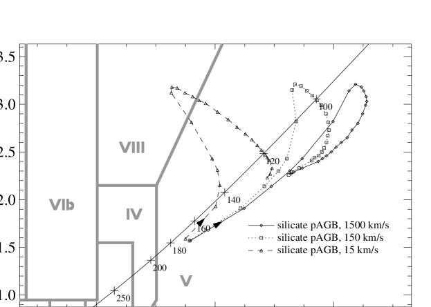
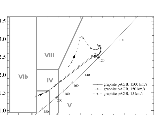
Figure 7: In these IRAS colour-colour diagrams, the effect of different velocities of the post-AGB wind with dust formation is presented. The 15 km s^-1, 150 km s^-1 and 1500 km s^-1 models are calculated in runs 1, 4 and 6. The upper diagram shows the silicate models, the lower diagram the graphite models. The graphite 15 km s^-1 track starts at 6200 K, all others at 6050 K.

4.2 Carbon-rich dust

Let us now turn to the models with carbon-rich dust. This type of dust is a more efficient absorber than silicate dust as can be seen in Fig. 4. The visual magnitude is larger than for the oxygen rich models, reflecting a larger circumstellar extinction in the Johnson V band. One can also see that the infrared energy output is larger.

The beginning of the track of the carbon-dust models in the colour-colour diagram (Fig. 3) is located at a higher colour temperature than for the oxygen-rich models because more energy is absorbed by the dust. At first, the track moves to lower temperatures, and as the star begins to evolve more rapidly, the curve makes a slight backward loop in the diagram due to the heating of the shell. Then, contrary to the silicate model, the shell cools again.

This somewhat unexpected result can be explained by the properties of the absorbing material. It is instructive to investigate the effective cross section $Q_{0}$ of the two grain species as a function of the effective temperature of the central star spectrum (i.e. a blackbody). $Q_{0}$ is defined as

$$Q_{0}=\frac{\int_{0}^{\infty}B_{\nu}(T_{\rm eff})\alpha_{\nu}{\rm d}\nu}{\int_{0}^{\infty}B_{\nu}(T_{\rm eff}){\rm d}\nu}$$ (9)

With $B_{\nu}$ the blackbody intensity distribution and $\alpha_{\nu}$ the absorption cross section of the grains. The formula is chosen in such a way that the total energy absorbed by the grains is proportional to $L\times Q_{0}$. Note that $L$ is constant during the evolution. The absorption coefficients have been chosen such that both grain species have the same dust-to-gas mass ratio. The resulting curves are shown in Fig. 8

Figure 8: The effective cross section for the grain species used in our study as a function of the effective temperature of a blackbody. The total luminosity of the central source remains constant and the dust-to-gas mass ratio for both grain species is equal.

For temperatures between approximately 1000 K and 50 000 K silicates absorb less energy than graphite. It can be a factor of 10 lower in the temperature range for cool post-AGB stars. This is caused by the fact that silicates are inefficient absorbers at optical wavelengths. From these results we can expect that for temperatures between 10 000 K and 50 000 K the total IR emission of silicates will rise much more drastically than for graphite. For temperatures above 50 000 K the peak of the energy distribution shifts into the EUV. At these wavelengths silicates are more efficient absorbers and we can see that for these temperatures the total amount of energy absorbed by the silicates is higher than for graphite.

Thus, in the last data points of the track in the IRAS colour-colour diagram, the absorption efficiency of graphite does increase less strongly with rising effective temperature. In this case, the interplay between the evolving star (now heating up the shell less rapidly) and the expanding shell (giving rise to cooling) has as a result that the expanding shell becomes the more dominant factor and consequently the shell cools. In Fig. 4 these two effects are illustrated by the decreasing IRAS fluxes.

4.2.1 Dust formation in the post-AGB wind

In contrast to oxygen-rich dust, graphite has no feature in the IRAS 12 $\mu$m pass band. Also the shape for the emissivity law of graphite is such that the hot dust peaks at near-infrared wavelengths, contributing negligibly to the 12 $\mu$m band (Figs. 4 and 6). Therefore one does not expect a large effect of the hot dust on the IRAS 12 $\mu$m flux. However, the 12 $\mu$m, 25 $\mu$m and 60 $\mu$m flux densities of these models are lower than for the corresponding AGB-only dust formation models (Fig. 4). This stems from the fact that the hot dust absorbs a large fraction of the stellar energy, yielding a cooler AGB shell.

4.2.2 Different post-AGB wind velocities

The effect of the post-AGB outflow velocity on the graphite models is presented in the lower panel of Fig. 7. The 1500 km s^-1 track behaves almost the same as the 150 km s^-1 track and the track without post-AGB dust. The 15 km s^-1 track however is different, first it moves upward, then bends downward and finally makes the counter-clockwise loop. The initial increase in the [25]–[60] colour is caused by the fact that the large amount of hot dust now shields the AGB shell more efficiently, making the AGB shell even cooler than previously. As the star becomes hotter, the dust condensation radius moves rapidly outward, making shielding less efficient. The AGB shell now obtains more energy from the central star and heats up, resulting in higher [25]–[60] temperatures. The tracks evolve asymptotically towards each other and finally the counter-clockwise loop sets in, as was already explained.

4.3 Constant mass loss

In Fig. 9 the silicate tracks for run 4 (decreasing AGB mass loss) and run 3 (constant mass loss) in the IRAS colour-colour diagram are shown. Both the [12]–[25] and the [25]–[60] colour temperature of the constant mass loss track are slightly higher than for the decreasing mass loss track.

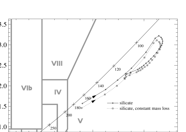
Figure 9: IRAS colour-colour diagram in which the difference between the decreasing and constant mass loss (runs 4 and 3) are shown for the silicate tracks. The first data point for both tracks is the $T_{\rm eff}$ = 6050 K model.

The constant mass loss creates relatively more cool dust further from the star. This cooler dust emits less radiation and therefore the hotter dust at the inner parts of the AGB shell (where the mass loss rates for both tracks are the same) will dominate the spectrum more. This gives the result that the integrated spectrum of all dust appears hotter. This effect is strongest at 60 $\mu$m, less at 25 $\mu$m and absent at 12 $\mu$m. As a whole, the effect of different AGB mass loss rates is small. The effect on the graphite tracks is basically the same and is not shown.

4.4 Different end of the AGB

For all the models that have been discussed so far, it was assumed that the transition mass loss starts at $P_{\rm a}$ = 100 d, and that the Reimers mass loss starts at $P_{\rm b}$ = 50 d. However, the evolutionary behaviour of the calculated models strongly depends on the exact moment of ‘superwind’ cessation (Szczerba 1993). In this section, we will present an investigation into the effect of changing this unknown parameter.

As stated before, the evolution of the central star in the ($P_{\rm a}$,$P_{\rm b}$) = (100d,50d) and the ($P_{\rm a}$,$P_{\rm b}$) = (125d,75d) models is identical after $T_{\rm eff}$ = 6042 K. However, the density structure of the circumstellar shell is entirely different when the star has reached this temperature. Whereas the ($P_{\rm a}$,$P_{\rm b}$) = (100d,50d) model then barely has a detached shell, the ($P_{\rm a}$,$P_{\rm b}$) = (125d,75d) model already has a shell with a kinematic age in excess of 4500 yr, which has much cooler dust.

We will now look at the results for this run in the colour-colour diagram. It appears that the alternative end of the AGB entirely changes the path in the colour-colour diagram (Fig. 10). A selection of spectral energy distributions is presented in Fig. 11.

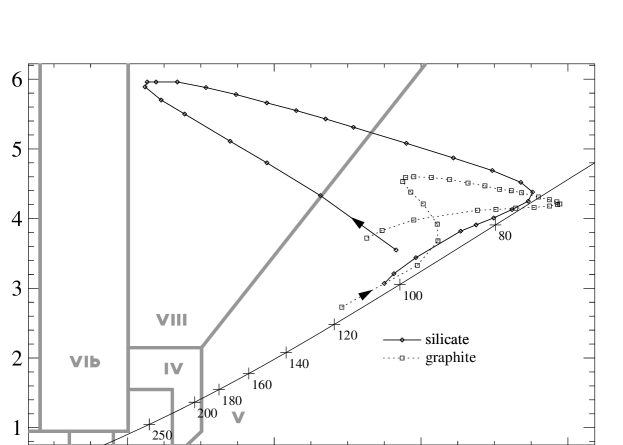
Figure 10: IRAS colour-colour diagram for the models without post-AGB dust formation in run 5, the case with an earlier start of the transition phase than in run 4. The first data point for both tracks is the $T_{\rm eff}$ = 5450 K model.

Figure 11: The spectral energy distribution at several stages during the post-AGB evolution for an earlier start of the transition phase (run 5). The upper panel shows the SED for silicate dust without post-AGB dust formation, the lower panel for graphite without post-AGB dust formation. The flux densities are calibrated for an assumed distance of 1 kpc. The temperatures are indicated.

From the start, the silicate dust track moves strongly to the upper left, making a turn to the lower right, and finally a bend to the left. Since the star evolves slowly (it takes approximately 750 yr to go from 5450 K to 5500 K), the circumstellar shell cools rapidly, and only the stellar photosphere is visible at 12 $\mu$m (Fig. 11). This is reflected in an increasing [12]–[25] colour temperature: the photospheric 12 $\mu$m flux remains approximately the same, while the 25 $\mu$m flux and the [25]–[60] temperature decrease due to the cooling of the shell. Subsequently the star starts to evolve more rapidly than the shell expands, and the [12]–[25] colour temperature decreases. This is due to the fact that the shell now heats up, increasing the 25 $\mu$m flux and decreasing the [25]–[60] colour, contrary to the 12 $\mu$m band which is still dominated by the decreasing photospheric emission of the evolving star. The shell continues to heat up, and the dust emission at 12 $\mu$m overtakes the decreasing photospheric flux density. The curve bends to higher [12]–[25] temperatures. The contribution of nebular bound-free emission at 12 $\mu$m for the hottest models increases the [12]–[25] colour temperature even more, and the track makes the, now familiar, clockwise loop.

All effects outlined above appear less strong for the carbon-rich model. It initially starts on a cooling curve, and later bends to the clockwise loop. This is explained by the fact that the dust emission from the carbon grains still is present at 12 $\mu$m in the first points, so that the shell cools in all colours. For the remainder of the evolution there always remains some dust emission in the 12 $\mu$m band, making the loop to the left less pronounced.

4.5 A near-IR colour-colour diagram

In this section we present the evolution of a post-AGB star in a colour-colour diagram which uses colours at shorter wavelengths: the K–[12] vs. [12]–[25] diagram. This diagram gives a different view of the evolution since in all models the Johnson K band will be dominated either by the stellar continuum or the bound-free emission of the ionized part of the nebula. Only in the models containing hot graphite grains, part of the flux in this band will originate from the grains. So, contrary to the IRAS colour-colour diagram which we presented earlier, this diagram contains information both on the central star and the dust. The results for run 4 are shown in Fig. 12, giving both the tracks using silicate and graphite grains and both the tracks assuming AGB-only and post-AGB dust formation.

Figure 12: The near-IR colour-colour diagram at several stages during the post-AGB evolution for run 4. For reference a blackbody curve is also included in the diagram.

The first thing we notice is that all four tracks, at least in a qualitative sense, look quite similar. This suggests that this colour-colour diagram is less sensitive to particulars of the grain emission and thus that the information on the evolution of the central star and the nebula is less ‘contaminated’ when compared with the IRAS colour-colour diagram. We have only investigated this for the 3 M_⊙ track and it is not yet clear if this observation is valid in a more general context. In the past years the IRAS colour-colour diagram has proven to be a very useful tool for studying post-AGB evolution. Our knowledge has increased considerably since its introduction. However, when we try to understand the details of this evolution better, the information from the IRAS colour-colour diagram becomes more and more confusing. The K–[12] vs. [12]–[25] diagram may be a valuable additional tool for the study of post-AGB evolution.

We will only discuss the evolution of the K–[12] colour in Fig. 12 since the evolution of the [12]–[25] colour already has been discussed earlier. At first both the flux in the K band and the 12 $\mu$m band are decreasing. However the 12 $\mu$m flux decreases more rapidly and therefore K–[12] evolves towards hotter colours. This can be understood if we realize that the central star heats up relatively slowly while the circumstellar shell expands relatively rapidly. At a temperature of around 8000 K the central star evolution will speed up considerably, reversing the preceding argument. The flux in the K band continues to drop, while the flux in the 12 $\mu$m band increases now, resulting in ever cooler K–[12] colours. This evolution continues until the central star starts to ionize a considerable part of the circumstellar shell and the K band flux will start to rise again due to nebular bound-free emission. This rise is so rapid that it reverses the evolution of the K–[12] colour.

The tracks for silicate and graphite grains are qualitatively similar, but are offset with respect to each other. This is mainly due to the different absorption efficiency of silicate and graphite grains (see Section 4.2). The difference between the silicate track with and without post-AGB dust formation can be understood solely from the presence or absence of the 10 $\mu$m emission feature. The difference between the graphite tracks with and without post-AGB dust formation stems from the fact that the hot dust in the post-AGB section of the wind mainly radiates around 3 $\mu$m and thus contributes to the K band flux.

5 Discussion and conclusions

In this paper we have presented a new model to calculate the spectral evolution of a hydrogen burning post-AGB star. The main new ingredient of this model is the possibility of extracting timescales of the post-AGB central star evolution from the most recent evolutionary calculations. Hence, contrary to previous studies, it is possible now to investigate other AGB and/or post-AGB mass loss rates and different prescriptions for the start of the post-AGB phase. The use of a photo-ionization code in which a dust code is built in, gives us the opportunity to study the evolution of the infrared emission of the circumstellar material.

We have performed a parameter study on a typical post-AGB star with a core mass of 0.605 M_⊙ taken from Blöcker (1995b). By varying the parameters that govern the mass loss and the evolutionary timescales of the post-AGB phase by a reasonable amount we find that:

1. The influence of the evolving star on the infrared colour evolution can not be neglected. In particular, the phase wherein the circumstellar shell can be considered as a stationary shell around a star that rapidly increases in temperature results in clockwise loops in the IRAS colour-colour diagram. This was not observed in many previous studies in which the temperature of the central star was taken to be constant. Instead, in these studies the evolutionary path followed a counter-clockwise loop in the colour-colour diagram because of the inevitable cooling of the shell.
   Only Szczerba & Marten (1993) who used a Blöcker track obtained a roughly similar result with their dust radiative transfer code. Volk (1992) found a slight deviation from the counter-clockwise loop in the colour-colour diagram. He used the coarse grid of evolutionary timescales from the 0.644 M_⊙ Schönberner (1983) track. The output of the photo-ionization code cloudy was used as input for a dust radiative transfer model. It is not clear to what extent that choice influenced the path followed in the IRAS colour-colour diagram.
   The crucial influence of the evolution of the central star warrants further parameter studies with other stellar models, where the increase in temperature as a function of time will be different. It is expected that the heating of the shell will be more important for more rapidly evolving (i.e. larger core mass) stars.

2. The tracks that are followed in the IRAS colour-colour diagram are very sensitive to the adopted dust opacity law and solid state features. Two main differences between the silicate and graphite models that were studied are evident. Firstly the IRAS colours of the silicate models are very sensitive to newly synthesized dust in the post-AGB wind because of the silicate 10 $\mu$m feature that contributes significantly to the 12 $\mu$m flux density. In contrast, hot graphite dust emits mainly shortward of the 12 $\mu$m pass band and thus post-AGB dust formation has less influence in this case. Secondly, the dependency of the absorption efficiency on the central star temperature is much stronger for silicates than for graphite in the temperature regime studied here. Therefore silicates react much stronger to the heating of the central star and thus give rise to much larger loops in the IRAS colour-colour diagram.
   Our knowledge of dust opacities, and certainly of solid state features in the mid- and far-infrared, will improve when the results of the ISO mission have been digested (Waters et al. 1996). For example, the well-known 21 $\mu$m and 30 $\mu$m features that have been observed in the infrared spectrum of carbon-rich post-AGB stars and planetary nebulae (e.g. Omont et al. 1995) have not been taken into account in this study. In addition, the wavelength coverage up to 200 $\mu$m will be of great help to determine the wavelength dependence of the dust opacities towards long wavelengths.

3. A third decisive factor that governs the evolution of the IRAS colours is the definition of the end of the AGB. The sooner an object enters the transition phase, i.e. the sooner the heavy AGB mass loss ceases, the longer the evolution to higher effective temperatures will last. This results in cool circumstellar dust shells, and consequently these models are on a location in the IRAS colour-colour diagram where not many post-AGB stars were expected previously. In this respect it is noteworthy to refer to Fig. 10 where oxygen-rich post-AGB stars are predicted to be present in the upper part of region VIII. A re-investigation of the sources in that region would be useful in testing whether this scenario is realistic.

4. Changing the mass loss prescription in the coolest part of the AGB evolution that we considered has little influence on the IRAS colours of the models.

In general we find that the variation of the parameters mentioned above, which are still not very well determined, result in a variety of different paths in the IRAS colour-colour diagram. This is certainly part of the explanation why planetary nebulae do not occupy a well-structured region in the IRAS colour-colour diagram (cf. Volk 1992). As a by-product of this investigation we find that the same location in the IRAS colour-colour diagram can be occupied by objects with an entirely different evolutionary past. Apparently, the location in the IRAS colour-colour diagram can not a priori give a unique determination of the evolutionary status of an object.

As an alternative to the IRAS colour-colour diagram, the K–[12] vs. [12]–[25] colour diagram is presented. The tracks in this diagram seem less affected by particulars of the grain emission. Hence this diagram might prove to be a valuable additional tool for studying post-AGB evolution.

The feedback of observational work, after a sufficient number of parameter studies, will be of help to assess the selection effects in our post-AGB sample selection criteria, and will give constraints on the assumptions that now have to be made on the central star and nebular evolution.

References

- [1983] Aller L.H., Czyzak S.J., 1983, ApJS, 51, 211
- [1999] Blöcker T., 1995a, A&A, 297, 727
- [1999] Blöcker T., 1995b, A&A, 299, 755
- [1999] Blöcker T., Schönberner D., 1991, A&A, 244, L43
- [1999] Bowen G.H., 1988, ApJ, 329, 299
- [1993] Ferland G.J., 1993, University of Kentucky Physics Department Internal Report
- [1999] Fernie J.D., 1995, AJ, 110, 3010
- [1999] Fernie J.D., Sasselov D.D., 1989, PASP, 101, 513
- [1999] Frank A., Balick B., Icke V., Mellema G., 1993, ApJ, 404, L25
- [1999] Górny S.K., Tylenda R., Szczerba R., 1994, A&A, 284, 949
- [1999] Groenewegen M.A.T., de Jong T., 1993, A&A, 267, 410
- [1999] Groenewegen M.A.T., de Jong T., 1994, A&A, 283, 463
- [1985] Hrivnak B.J., Kwok S., Volk K.M., 1989, ApJ, 346, 265
- [1999] Kurucz R.L., 1991, Rev. Mex. Astron. Astrofís., 23, 181
- [1999] Lèbre A., Mauron N., Gillet D., Barthès D., 1996, A&A, 310, 923
- [1999] Loup C., 1991, PhD Thesis, University of Grenoble
- [1999] Marten H., Schönberner D., 1991, A&A, 248, 590
- [1999] Marten H., Szczerba R., Blöcker T., 1993, in Weinberger R., Acker A., eds, IAU Symp. 155: Planetary Nebulae. Kluwer Academic Publishers, Dordrecht, p.363
- [1991] Martin P.G., Rouleau F., 1991, in Malina R.F., Bowyer S., eds, Extreme Ultraviolet Astronomy. Pergamon Press, Oxford, p.341
- [1977] Mathis J.S., Rumpl W., Nordsieck K.H., 1977, ApJ, 217, 425
- [1999] Mellema G., 1993, PhD Thesis, University of Leiden
- [1999] Olofsson H., 1993, in Schwarz H.E., ed., Second ESO/CTIO workshop, Mass loss on the AGB and beyond. ESO Conference and Workshop Proceedings No. 46, Garching, p.330
- [] Omont A., Moseley S.H., Cox P. et al., 1995, ApJ, 454, 819
- [1999] Ostlie D.A., Cox A.N., 1986, ApJ, 311, 864
- [1999] Oudmaijer R.D., 1996, A&A, 306, 823
- [1999] Oudmaijer R.D., Bakker E.J., 1994, MNRAS, 271, 615
- [1999] Oudmaijer R.D., van der Veen W.E.C.J., Waters L.B.F.M., Trams N.R., Waelkens C., Engelsman E., 1992, A&AS, 96, 625
- [1999] Oudmaijer R.D., Waters L.B.F.M., Pottasch S.R., 1993, in Schwarz H.E., ed., Second ESO/CTIO workshop, Mass loss on the AGB and beyond. ESO Conference and Workshop Proceedings No. 46, Garching, p.122
- [1999] Oudmaijer R.D., Waters L.B.F.M., van der Veen W.E.C.J., Geballe T.R., 1995, A&A, 299, 69
- [1999] Pauldrach A., Puls J., Kudritzki R.P., Méndez R.H., Heap S.R., 1988, A&A, 207, 123
- [1999] Pottasch S.R., 1984, Planetary Nebulae. Reidel Publishing Company, Dordrecht
- [1999] Reimers D., 1975, Mem. Soc. Sci. Liège, 8, 369
- [1999] Schönberner D., 1979, A&A, 79, 108
- [1999] Schönberner D., 1981, A&A, 103, 119
- [1999] Schönberner D., 1983, ApJ, 272, 708
- [1999] Schönberner D., Blöcker T., 1993, in Sasselov D.D., ed., Luminous High-Latitude Stars. A.S.P. Conference Series Vol. 45, p.337
- [1999] Siebenmorgen R., Zijlstra A.A., Krügel E., 1994, MNRAS, 271, 449
- [] Slijkhuis S., 1992, PhD Thesis, University of Amsterdam
- [1999] Slijkhuis S., Groenewegen M.A.T., 1992, in Slijkhuis S., PhD Thesis, University of Amsterdam, Chapter 6
- [1999] Straižys V., Kuriliene G., 1981, Ap&SS, 80, 353
- [1999] Szczerba R., 1993, in Weinberger R., Acker A., eds, IAU Symp. 155: Planetary Nebulae. Kluwer Academic Publishers, Dordrecht, p.350
- [1999] Szczerba R., Marten H., 1993, in Schwarz H.E., ed., Second ESO/CTIO workshop, Mass loss on the AGB and beyond. ESO Conference and Workshop Proceedings No. 46, Garching, p.90
- [1999] Trams N.R., Waters L.B.F.M., Waelkens C., Lamers H.J.G.L.M. van der Veen W.E.C.J., 1989, A&A, 218, L1
- [] Trams N.R., Waters L.B.F.M., Lamers H.J.G.L.M., Waelkens C., Geballe T.R., Thé P.S., 1991, A&AS, 87, 361
- [] van der Veen W.E.C.J., Habing H.J., 1988, A&A, 194, 125
- [1999] van der Veen W.E.C.J., Habing H.J., Geballe T.R., 1989, A&A, 226, 108
- [1999] Van de Steene G.C., van Hoof P.A.M., 1995, in Van de Steene G.C., PhD Thesis, University of Groningen, Chapter 7
- [1999] Van de Steene G.C., Jacoby G.H., Pottasch S.R., 1996, A&AS, 118, 243
- [1999] van Hoof P.A.M., Trams N.R., Waelkens C., Cassatella A., 1991, in Trams N.R., PhD thesis, University of Utrecht, Chapter 7
- [1999] Vassiliadis E., Wood P.R., 1993, ApJ, 413, 641
- [1999] Vassiliadis E., Wood P.R., 1994, ApJS, 92, 125
- [1999] Volk K., 1992, ApJS, 80, 347
- [1999] Volk K.M., Kwok S., 1989, ApJ, 342, 345
- [1999] Waelkens C., Van Winckel H., Bogaert E., Trams N.R., 1991, A&A, 251, 495
- [1999] Waelkens C., Van Winckel H., Trams N.R., Waters L.B.F.M., 1992, A&A, 256, L15
- [1999] Waters L.B.F.M., Molster F.J., de Jong T. et al., 1996, A&A, 315, L361
- [1999] Wood P.R. 1990, in Mennessier M.O., Omont A., eds, From Miras to Planetary Nebulae: Which Path for Stellar Evolution?. Editions Frontières, Gif sur Yvette, p.67