A Neural Network-based ARX Model of Virgo Noise.

Abstract

In this paper a Neural Networks based approach is presented to identify the noise in the VIRGO context. VIRGO is an experiment to detect Gravitational Waves by means of a Laser Interferometer. Preliminary results appear to be very promising for data analysis of realistic Interferometer outputs.

1 Introduction

Neural Networks (NN’s) have become in the last years a very effective instrument for solving many difficult problems in the field of Signal Processing due to their properties like non-linear dynamics, adaptability, self-organization and high speed computational capability (see for example [4] and the papers therein quoted).

Aim of this paper is to show the feasibility of the use of NN’s to solve difficult problems of signal processing regarding the so called VIRGO project. Gravitational Waves (GW’s) are travelling perturbations of the space-time predicted by the theory of  General Relativity, emitted when massive systems are accelerated. Up to now, there is only an indirect evidence of their existence, obtained by the observations of the binary pulsar system PSR 1913+16. Moreover, the direct detection of GW’s is not only a relevant test of General Relativity, but the start of a new picture of the Universe. In fact, GW’s carry complementary information with respect to electromagnetic and optical waves, since the GW’s are practically not absorbed by the matter.

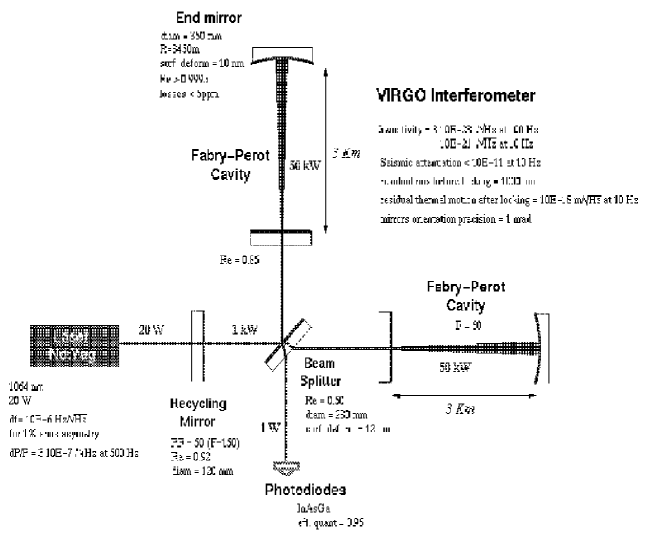
Figure 1: Scheme of the Virgo interferometer.

The aim of the Virgo experiment is the direct detection of gravitational waves and, in joint operation with other similar detectors, to perform gravitational waves astronomical observations. In particular, the VIRGO project is designed for broadband detection from $10Hz$ to $10kHz$. The principle of the detector is shown in figure 1.

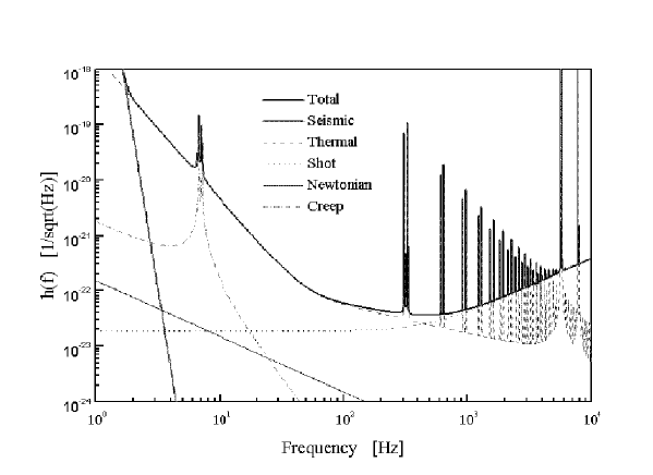
Figure 2: Sensitivity curve of the Virgo interferometer.

A $3$ $km$ arm-length Michelson interferometer with suspended mirrors (test masses) is used. The phase difference $\Delta\phi$ between the two arms is amplified using Fabry-Perot cavities of Finesse $50$ in each arm. Aiming for detection sensitivity of $3.10E-23\frac{1}{Hz}\quad at\quad 100Hz$, VIRGO is a very delicate experimental challenge because of the competition between various sources of noise and the very small expected signal. In fact, the interferometer will be tuned on the dark fringe, and then the signal to noise ratio will be mainly limited, in the above defined range of sensitivity, by residual seismic noise, thermal noise of the suspensions photon counting noise (shot noise). In figure 2 the overall sensitivity of the apparatus is shown. In this figure it is easy to see the contribution of the different noise sources to the global noise.

In this context we use a Multi-Layer Perceptron (MLP) NN with the back-propagation learning algorithm to model and identify the noise in the system, because we experimentally found that FIR NN’s and Elman NN’s did not work in a satisfying manner.

Both the FIR [11] and Elman [12] models proved to be very sensible to overfitting and were not stable. Furthermore the Elman network required a great number of hidden units, while the FIR network required a great number of delay terms. Instead, the MLP proved succesfull and easy to train because we used the Bayesian learning paradigm.

2 Neural networks for time-domain system identification

NN’s are massively parallel, distributed processing systems. They are composed of a large number of processing elements (called nodes, units or neurons) which operate in parallel. Scalars (called weights) are associated to the connections between units and determine the strength of the connections themselves. Computational capability is due to the connections between the units and to their collective behaviour. Furthermore, information representation is distributed, i.e. no single unit is charged with specific information. NN’s are well-known for their universal approximation capability [1].

System identification consists in finding the input-output mapping of a dynamic system. A discrete-time Multi-Input Multi-Output (MIMO) system (or a continuous-time sampled-data system) can be described with a set of non-linear difference equations of the form (input-state-output representation):

$$\left\{\begin{array}[]{ll}{\bf z}(n+1)=F({\bf z}(n),{\bf u}(n))&\\ {\bf y}(n)=G({\bf z}(n))&\end{array}\right.$$ (1)

where ${\bf z}\in R^{L}$ is the state vector of the system, ${\bf u}\in R^{M}$ is the input vector and ${\bf y}\in R^{N}$ is the output vector. Since we can not always access the state vector of the system, therefore we can use an input-output representation of the form:

$${\bf y}(n) = {\cal F}[{\bf y}(n-1),{\bf y}(n-2),\ldots,{\bf y}(n-n_{y}),$$ (2)

$${\bf u}(n-n_{d}),\ldots,{\bf u}(n-n_{u}-n_{d}+1)]$$

where $n_{u}$ and $n_{y}$ are the maximum lags of the input and output vectors, respectively, and $n_{d}$ is the pure time-delay (or dead-time) in the system. This is called an ARX model (autoregressive with exogenous inputs,) and it can be shown that a wide class of discrete-time systems can be put in this form [2]. To build a model of the form (2), we must therefore obtain an estimation of the functional ${\cal F}[\cdot]$, which generally is nonlinear.

Given a set of input-output pairs, a neural network can be built [4] which approximates the desired functional ${\cal F}[\cdot]$. Such a network has $n_{y}N+(n_{u}-n_{d})M$ inputs and $N$ outputs (see figure 3).

A difficulty in this approach arises from the fact that generally we do not have information about the model order (i.e. the maximum lags to take into account) unless we have some insight into the system physics. Furthermore, the system is non-linear. Recently [3] a method has been proposed for determining the so-called embedding dimension of nonlinear dynamical systems, when the input-output pairs are affected by very low noise. Furthermore, the lags can be determined by evaluating the average mutual information (AMI)[8]. Such methodologies, although not always successful, can be nevertheless used as a starting point in model design.

3 Virgo

In the VIRGO data analysis, the most difficult problem is the gravitational signal extraction from the noise due to the intrinsic weakness of the gravitational waves, to the very poor signal-to-noise ratio and to their not well known expected templates. Furthermore, the Virgo detector is not yet operational, and the noise sources analyzed are purely theoretical models (often stationary noises), not based on experimental data. Therefore, we expect a great difference between the theoretical noise models and the experimental ones. As a consequence, it is very important to study and to test algorithms for signal extraction that are not only very good in signal extraction from the theoretical noise, but also very adaptable to the real operational conditions of Virgo.

For this reason, we decided the following strategy for the study, the definition and the tests of algorithms for gravitational data analysis. The strategy consists of the following independent research lines.

The first line starts from the definition of the expected theoretical noise models. Then a signal is added to the Virgo noise generated and the algorithm is used for the extraction of the signal of known and unknown shape from this noise at different levels of signal-to-noise ratio. This will allow us to make a number of data analysis controlled experiments to characterize the algorithms.

The second line starts from the real measured environmental noise (acoustic, electromagnetic, …) and tries to identify the noise added to a theoretical signal. In this way we can test the same algorithms in a real case when the noise is not under control.

Using this strategy, at the end, when in a couple of years Virgo will be ready for the first test of data analysis, the procedure will be moved to the real system, being sure to find small differences from theory and reality after having acquired a large experience in the field.

4 A neural network-based model of the Virgo system

As we have seen in the introduction, the Virgo interferometer can be characterized by a sensitivity curve, which expresses the capability of the system to filter undesired influences from the environment, and which could spoil the detection of gravitational waves (such a noise is generally called seismic noise). The sensitivity curve has the following expression:

$$S(f)=\left\{\begin{array}[]{ll}\frac{S_{1}}{f^{5}}+\frac{S_{2}}{f}+S_{3}\left[1+\left(\frac{f}{f_{k}}\right)^{2}\right]+S_{\nu}&\quad f\geq f_{\textrm{min}}\\ S(f_{\textrm{min}})&\quad f<f_{\textrm{min}}\end{array}\right.$$ (3)

where:

• $f_{\textrm{min}}=4Hz$

• $f_{k}=500Hz$ is the shot noise cut-off frequency

• $S_{1}=1.8\cdot 10^{-36}$ is the pendulum mode

• $S_{2}=0.33\cdot 10^{-42}$ is the mirror mode

• $S_{3}=3.24\cdot 10^{-46}$ is the shot noise

The contribution $S_{\nu}(f)$ of violin resonances is given by:

$$S_{\nu}(f)=\sum_{i}^{n}\frac{1}{i^{4}}\frac{f_{i}^{(c)}}{f}\frac{C_{c}\phi_{i}^{2}}{\left[\left(\frac{f}{if_{i}^{(c)}}\right)^{2}-1\right]^{2}+\phi_{i}^{2}}+\frac{1}{i^{4}}\frac{f_{i}^{(f)}}{f}\frac{C_{f}\phi_{i}^{2}}{\left[\left(\frac{f}{if_{i}^{(f)}}\right)^{2}-1\right]^{2}+\phi_{i}^{2}}$$ (4)

where the different masses of close and far mirrors are taken into account:

• $f_{i}^{(c)}=i\cdot 327Hz$

• $f_{i}^{(f)}=i\cdot 308.6Hz$

• $C_{c}=3.22\cdot 10^{-40}$

• $C_{f}=2.82\cdot 10^{-40}$

• $\phi_{i}^{2}=10^{-7}$

Note that we used a simplified curve for our simulations, in which we neglected the resonances (see figure 4).

Samples of the sensitivity curve $\{S_{i}\}_{i}$ can be obtained by evaluating the expression (3) at a set of frequencies $\{f_{i}\}_{i}$, $f_{i}\in[10,10000]$. The samples of the sensitivity curve allow us to obtain the system transfer function (in the frequency domain), $N(j2\pi f)$, such that:

$$|N(j\omega)|^{2}=S(j\omega)$$ (5)

¿From this, by means of an inverse Discrete Fourier Transform, samples of the system transfer function (in the time domain) can be obtained. Our aim is to build a model of the system transfer function (5).

Assuming that the interferometer input noise is a zero mean Gaussian process, by feeding it to the system (i.e. filtering it through the system transfer function) we obtain a coloured noise. The so obtained white noise-colored noise pairs can then be used to train an MLP, as shown in figure 3.

4.1 Experimental Results

The first step in building an ARX model is the model order determination. To determine suitable lags which describe the system dynamics, we used the AMI criterion [8]. This can be seen as a generalization of the autocorrelation function, used to determine lags in linear systems. A strong property of the AMI statistic is that it takes into account the non-linearities in the system. Usually, the lag is chosen as the first minimum of the AMI function. The result is reported in figure 5, in which the first minimum is at 1. To find how many samples are necessary to unfold the (unknown) state-space of the model (the so called embedding dimension [8]) we used the method of [3], the Lipschitz decomposition. The result of the search is reported in figure 6.

From the figure we can see that, starting from lag three, the order index decreases very slowly, and so we can derive that the width of the input window is at least three. In order to test the NN’s capability in solving the problem, we chose a width of 5, both for input and output (i.e. $n_{y}=n_{u}=5$). In this way, we obtained a NN with a simple structure. Furthermore, some preliminary experiments showed that the system dead-time is $n_{d}=0$; this gives the best description of the system dynamics.

Another fundamental issue is the NN complexity, i.e. the number of units in the hidden layers of the NN. Usually the determination of the network complexity is critical because of the risks of overfitting. Since the NN was trained following a Bayesian framework, then overfitting was of no concern; so we directed our search for a model with the minimum possible complexity. In our case, we found a hidden layer with 6 $tanh$ units is optimal.

The Bayesian learning framework (see [10] and [9]) allows the use of a distribution of NN’s, that is, the model is a realization of a random vector whose components are the NN weights. The so obtained NN is the most probable given the data used to train it. This approach avoids the bias of the cross-validatory techniques commonly used in practice to reduce model overfitting [6]. To allow for a smooth mapping which does not produce overfitting, several regularization parameters (also called hyperparameters) embedded in the error criterion have been used:

• one for each set of connections out of each input node,

• one for the set of connections from hidden to output units,

• one for each of the bias connections,

• one for the data-contribution to the error criterion.

Usually, the hyperparameters of the first three kinds are called alphas, while the last is called a beta.

The approach followed in the application of the Bayesian framework is the “exact integration” scheme, where we sample from the analytical form of the distribution of the network weights. This can be done if we assume an analytic form for the prior hyperparameters distribution, in particular a distribution uniform on a logarithmic scale:

$$p(\ln\alpha_{i})=\frac{1}{\alpha_{i}}.$$

This distribution is non-informative, i.e. it embodies our complete lack of knowledge about the values the hyperparameters should take.

The chosen model was trained using a sequence of little less than a million of patterns (we sampled the system at 4096Hz for 240s) normalized to zero mean and unity variance with a whitening process. Note that the input-output pairs were processed through discrete integrators to obtain pattern-target pairs, as shown in figure 3. The NN was then tested on a 120s long sequence.

The NN was trained for $370$ epochs, with the hyperparameters being updated every $15$ epochs. A close look at the $\alpha$ hyperparameters shows that all the inputs are relevant for the model (they are of the same magnitude; note that this further confirms the pre-processing analysis). The $\beta$ hyperparameter shows that the data contribution to the error is very small (as we would expect, since the data are synthetic).

The simulations were made using the MATLAB^© language, the Netlab Toolbox [7] and other software designed by us.

In figure 7, the PSDs of the target and the predicted time series are shown; in the lower part of the figure is reported the PSDs of the prediction residuals.

In figure 8, the PSD of a 100Hz sine wine added to the noise is shown, with the signal extracted by the network. As can be seen, the network recognizes the frequency of the sine wave with the maximum precision allowed by the residuals.

5 Conclusion

In this paper we have shown some preliminary tests on the use of NN’s for signal processing in the VIRGO Project. Some observations can be elicited from the experimental results:

• In evaluating the Power Spectral Densities (PSDs), we made the hypothesis that the system is sampled at $4096Hz$. It is only a work hypothesis, but it shows how the network reproduces the system dynamics up to $2048Hz$. Note that the PSDs are nearly the same also if we were near the Nyquist frequency.

• The PSD of the residuals shows a nearly-white spectrum, which is index of the model goodness (see [5]).

The next steps in the research are:

-

to increase the system model order and to test if there are significant differences in prediction;

-

to test the models with a greater number of samples to obtain a better estimate of the system dynamics;

-

to model the noise inside the system model to improve the system performance and to allow a multi-step ahead prediction (i.e. an output-error model)

Figure 3: A neural network ARX model.

Figure 4: The simplified sensitivity curve used for the experiments.

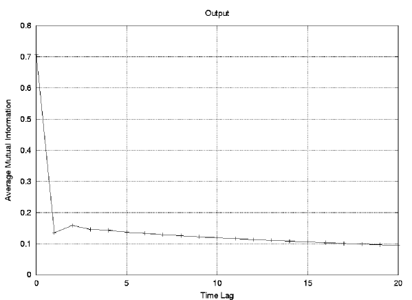
Figure 5: Average mutual information.

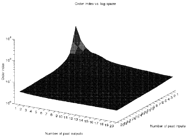
Figure 6: Determination of the embedding dimension.

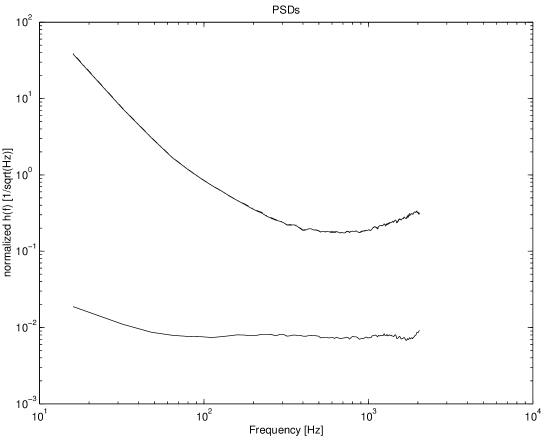
Figure 7: Results of the training.

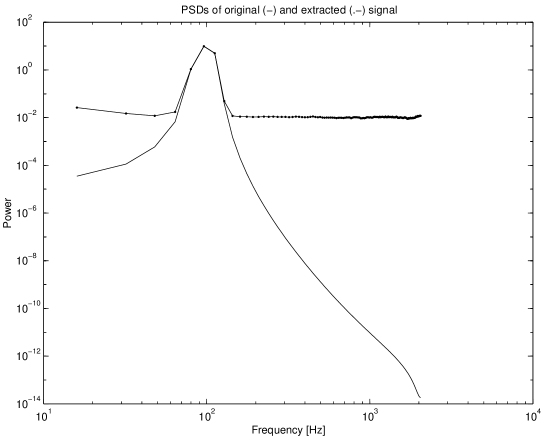
Figure 8: Example of signal extraction.

References

- [1] K. Hornik, M. Stinchcombe, H. White, “Multilayer Feedforward Networks are Universal Approximators”, Neural Networks, Vol. 2, pp. 359–366, 1989.
- [2] S. Chen, S. A. Billings, “Modelling and Analysis of Nonlinear Time Series”, Int. J. Control, Vol. 50, No. 6, pp. 2151–2171, 1989.
- [3] X. He, H. Asada, “A New Method for Identifying Orders of Input-Output Models for Nonlinear Dynamic Systems”, Proc. of the American Control Conf., San Francisco, California, 1993.
- [4] F. Luo, R. Unbehauen, “Applied Neural Networks for Signal Processing”, Cambridge University Press, Cambridge, 1997.
- [5] L. Ljung, “System Identification Toolbox User’s Guide”, The MathWorks Inc, 1995.
- [6] C. M. Bishop, “Neural Networks for Pattern Recognition”, Clarendon Press, Oxford, 1996.
- [7] C. M. Bishop, I. T. Nabney, Netlab Toolbox, Neural Computing Research Group, Aston University, Birmingham, 1996.
- [8] H. D. I. Abarbanel, “Analysis of Observed Chaotic Data”, Springer, 1996.
- [9] R. M. Neal, “Bayesian Learning for Neural Networks”, Ph.D. thesis, University of Toronto, Canada, 1994.
- [10] D. J. C. MacKay, “Hyperparameters: optimise or integrate out?”, Maximum Entropy and Bayesian Methods, Dordrecht, 1993
- [11] A. C. Tsoi, A. D. Back, “FIR and IIR synapses, a new neural network architecture for time series modelling”, Neural Computation Vol.3, No. 3, pp. 375–385, 1991
- [12] J. Elman, “Finding structure in time”, Cognitive Science Vol. 14, pp. 179–211, 1990