Perturbations in a coupled scalar field cosmology
Abstract
I analyze the density perturbations in a cosmological model with a scalar field coupled to ordinary matter, such as one obtains in string theory and in conformally transformed scalar-tensor theories. The spectrum of multipoles on the last scattering surface and the power spectrum at the present are compared with observations to derive bounds on the coupling constant and on the exponential potential slope. It is found that the acoustic peaks and the power spectrum are strongly sensitive to the model parameters. The models that best fit the galaxy spectrum and satisfy the cluster abundance normalization have field energy density and a scale factor expansion law ,
I Introduction
Perhaps the most important concept in modern cosmology is that fundamental physics, along with gravity, shapes the distribution of matter on very large scales. Fundamental physics enters in at least two distinct ways: through the potential of the inflationary field, which sets the initial conditions of the fluctuation field, and through the properties of the dark matter, which govern the evolution of the fluctuations up to the present. As a consequence, the imprint of the density fluctuations on the microwave background and on the galaxy distribution allows tests of basic laws of physics that, in many cases, could not be realized with any other mean.
An impressive array of different proposals have been formulated for as concerns the inflationary side of the story, that is, the initial conditions. So far, there is not an overwhelming reason to modify the simplest inflationary prescription of a flat spectrum, although several variations on the theme, like a small tilting (Lucchin & Matarrese 1985, Cen et al. 1992) or some break in the scale invariance (Gottloeber et al. 1994, Amendola et al. 1995) or the contribute of primordial voids (Amendola et al. 1996) cannot be excluded either.
Similarly, many theories have been proposed for as concerns the evolution of the fluctuations, trying to elucidate the nature and properties of the dark matter component. A partial list of the dark matter recipes includes the standard CDM and variations such as CDM plus a hot component (MDM), or plus a cosmological constant (CDM), or plus a scalar field ( CDM). The latter class of models, in particular, has been explored greatly in recent times, to various purposes. First, a light scalar field is predicted by many fundamental theories (string theory, pseudo-Nambu-Goldstone model, Brans-Dicke theory etc), so that it is natural to look at its cosmological consequences (Wetterich 1995, Frieman et al. 1995, Ferreira & Joyce 1998). Second, a scalar field may produce an effective cosmological constant, with the benefit that its dynamics can be linked to some underlying theory, or can help escape the strong constraints on a true cosmological constant (Coble, Dodelson & Frieman 1997, Waga & Miceli 1999). In turn, this effective cosmological constant can be tuned to explain the observation of an accelerated expansion (Perlmutter et al. 1998, Riess et al. 1998) and to fix the standard CDM spectrum as well (Zlatev et al. 1998, Caldwell et al. 1998, Perrotta & Baccigalupi 1999, Viana & Liddle 1998). Finally, even a small amount of scalar field density may give a detectable contribution to the standard CDM scenario, similar to what one has in the MDM model (Ferreira & Joyce 1998, hereinafter FJ).
In this paper we pursue the investigation of the effects of a scalar field in cosmology by adding a coupling between the field and ordinary matter. Such a coupling has been proposed and studied several times in the past (e.g. Ellis et al. 1989, Wetterich 1995) but, as far as we know, its consequences on the microwave background and on the power spectrum have not been determined. Scope of this paper is to solve the fluctuation equations for a coupled scalar field theory, and to compare with the already available data in the microwave sky and in galaxy surveys. We refer to this model as coupled CDM. Up to a conformal transformation, the model we study is equivalent to a non-minimal coupling theory in which the scalar field couples to gravity like in a Brans-Dicke Lagrangian; the perturbations in such models have been investigated by Chen & Kamionkowsky (1999) and Baccigalupi et al. (1999) in a background in which the scalar field acts like a dynamical cosmological constant (see also Uzan 1999). The model we present here is in fact more general, since a wide class of non-minimal coupling models can be recast in the form we study below (Amendola et al. 1993, Wetterich 1995, Amendola 1999).
There are several models of cosmological scalar field in the literature, essentially characterized by the scalar field potential and by the initial conditions. We can divide the models in two broad class: in the first one, the field potential energy dominates at the present, so that it resembles a cosmological constant. In the second one, the field kinetic energy is not negligible, and the field adds to the ordinary matter as an additional component, like in MDM models. To this second class belongs the model of FJ. They adopt an exponential potential for the scalar field, able to drive an attractor scaling solution which self-adjusts to the dominant matter component. In such a model, the density fraction of the field does not depends on the initial conditions, but is determined by the potential parameters. Therefore, the coincidence that the energy density in the field and in the matter components are comparable can be explained by the underlying physics (the field potential) rather than by the initial conditions. Although the coupling we will introduce can be applied to any scalar field model, we focus our attention in this paper on the exponential potential model of FJ. Beside being particularly simple, because of its attractor properties (Wetterich 1988, Ratra & Peebles 1988), such a model is also easily falsifiable, because the effect of the scalar field is important at all times (not just at the present as when the field acts as a cosmological constant), and therefore induces a strong effect on the cosmological sky. As a consequence, the constraints we derive on the model parameters are rather strong.
The same exponential potential also allows solutions which belong to the first class mentioned above, in which the field acts much like a cosmological constant, and drives at the present an accelerated expansion. These solutions, and their linear perturbations, have been studied by Viana & Liddle (1998) and Caldwell et al. (1998). The effect of adding a coupling to these models will be analyzed in a subsequent work.
II Coupled scalar field model
Consider two components, a scalar field and ordinary matter (e.g., baryons plus CDM) described by the energy-momentum tensors and . General covariance requires the conservation of their sum, so that it is possible to consider a coupling such that, for instance,
| (1) | |||||
| (2) |
Such a coupling arises for instance in string theory, or after a conformal transformation of Brans-Dicke theory (Wetterich 1995, Amendola 1999). It has also been proposed to explain ’fifth-force’ experiments, since it corresponds to a new interaction that can compete with gravity and be material-dependent. The coupling arises from Lagrangian terms of the form (Wetterich 1995)
| (3) |
where and is the ordinary matter field of mass , e.g., the nucleon field.
The specific coupling (2) is only one of the possible form. Non-linear couplings as or more complicate functions are also possible. Also, one can think of different coupling to different matter species, for instance coupling the scalar field only to dark matter and not to baryons. Such a species-dependent coupling has been proposed by Damour, Gibbons & Gundlach (1990), and shown to be observationally viable. Notice that the coupling to radiation (subscript ) vanishes, since Here we restrict ourselves to the simplest possibility (2), which is also the same investigated earlier by Wetterich (1995) and is the kind of coupling that arises from Brans-Dicke models. For instance, a field with coupling to gravity in the Lagrangian acquires, after conformal transformation, a coupling to matter of the form (2) with
| (4) |
in the limit of small positive coupling this becomes
| (5) |
There are several constraints on the coupling constant along with constraints on the mass of the scalar field particles, reviewed by Ellis et al. (1989). The constraints arise from a variety of observations, ranging from Cavendish-type experiments, to primordial nucleosynthesis bounds, to stellar structure, etc etc. Most of them, however, apply only if the scalar couples to baryons, which is not necessarily the case, and/or involve the mass of the scalar field particles, which is unknown. The most stringent bound, quoted by Wetterich (1995) amounts to
| (6) |
but again holds only for a coupling to baryons. Moreover, these constraints are local both in space and time, and could be easily escaped by a time-dependent coupling constant. In the following we leave therefore as a free parameter.
The constraints from nucleosynthesis refer to the energy density in the scalar component. This has to be small enough not to perturb element production, so that at the epoch of nucleosynthesis (Wetterich 1995, Sarkar 1996, FJ)
| (7) |
We will see that this bound is satisfied by all the interesting models.
There is an immediate consequence of the coupling for as concerns cosmology. The coupling modifies the conservation equation for the ordinary matter, leading to a different effective equation of state for the matter. This alters the scale factor expansion law in matter dominated era (MDE) from to , . In turn, this has three effects. First, the sound horizon at decoupling (when decoupling occurs in MDE) is modified with respect to the uncoupled case, being larger for and smaller in the opposite case, as we will show. This modifies the peak structure of the microwave background multipoles. Second, the epoch of matter/radiation equivalence moves to a later epoch if and to an earlier epoch in the opposite case. This shifts the range of scales for which there is the growth suppression of the sub-horizon modes in radiation dominated era (RDE), leading to a turnaround of the power spectrum on larger scales if (smaller if ). Finally, the different scale factor law modifies the fluctuation growth for sub-horizon modes in the MDE, generally reducing the growth for all values of . Similar effects have been observed by Chen & Kamionkowsky (1999) and Baccigalupi et al. (1999) in Brans-Dicke models. The next sections investigate these effects in detail.
III Background
Here we derive the background equations in the conformal FRW metric
| (8) |
The scalar field equation is
| (9) |
where , and we adopt the exponential potential
| (10) |
The matter (subscript ) and the radiation (subscript ) equations are
| (11) | |||||
| (12) |
Denoting with the conformal time today, let us put
| (13) |
Without loss of generality, the scalar field can be rescaled by a constant quantity, by a suitable redefinition of the potential constant . We put then . This gives
| (14) | |||||
| (15) |
The (0,0) Einstein equation can be written
| (16) |
The dynamics of the model is very simple to study in the regime in which either matter or radiation dominates. Assume that the dominant component has equation of state
| (17) |
Then, following Copeland et al. (1997) we define
| (18) |
and introduce the independent variable . Notice that and give the fraction of total energy density carried by the scalar field kinetic and potential energy, respectively . Then, we can rewrite the equations as (Amendola 1999)
| (19) | |||||
| (20) |
where the prime denotes here and where we introduce the adimensional constants
| (21) |
(in Amendola 1999 we defined one half of the definition above). Notice that in this simplified system with a single component, plus the scalar field, the constant is the coupling constant for the dominant component only, so that we are implicitly assuming during RDE. The system is invariant under the change of sign of and of . Since it is also limited by the condition to the circle , we limit the analysis only to the unitary semicircle of positive . The critical points, i.e. the points that verify , are scaling solutions, on which the scalar field equation of state is
| (22) |
the scalar field total energy density is , and the scale factor is
| (23) |
( being the time defined by ).
The system (20) with an exponential potential has up to five critical points, that can be classified according to the dominant energy density: one dominated by the scalar field total energy density, one in which the fractions of energy density in the matter and in the field are both non-zero, one in which the matter field and the field kinetic energy are both non-zero, while the field potential energy vanishes, and finally two dominated by the kinetic energy of the scalar field (at ) . The critical points are listed in Tab. I, where we put For any value of the parameters there is one and only one stable critical point (attractor). More details on the phase space dynamics in Amendola (1999) and, for , in Copeland et al. (1997).
2 Tab. I
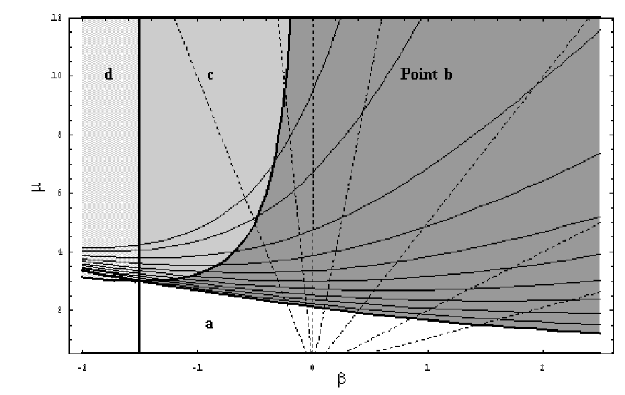
The perturbations on solutions converging toward the attractor have been studied in Viana & Liddle (1998) and in Caldwell et al. (1999) for zero coupling. In this case the scalar field is starting to dominate today, and mimics a cosmological constant. The case of interest here is instead the solution in Tab. I, since this is the only critical point which allow a partition of the energy between the scalar field and the matter and (contrary to ) is stable also in the RDE, when . The solution is compatible with a larger or smaller than . It exists and is stable (that is, is an attractor) in the region delimited by and and the two branches of the curve
| (24) |
The scale factor slope on the attractor is (Wetterich 1995)
| (25) |
and, if , is inflationary for
| (26) |
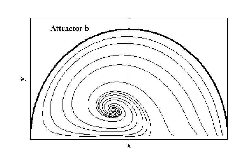
The parametric space region in which the attractor exists is shown in Fig. 1. For any value of the parameters there is a pair of observables . When radiation dominates, , and the scale factor is the usual RDE one, . The mapping from to is shown in the same Fig. 1: as one can see, to get a large a large is also needed. In Fig. 2 we show the phase space of the system for assuming matter domination. Notice that only for there is the possibility to get an inflationary attractor with , as some observations suggest. It can be easily demonstrated that the coupled exponential potential with is the only model that allows inflationary attractors with a non-vanishing matter component. Although such a possibility is intriguing, it is hardly realistic, since an inflationary expansion that lasted for most of the MDE would not allow any fluctuation growth via gravitational instability.
When both radiation and matter are present, the system goes rapidly from the radiation attractor, for which
| (27) |
to the matter attractor
| (28) |
It is convenient to note that is a measure of the deviation from the uncoupled law in MDE:
| (29) |
We give also the relation between the parameters and the observables
| (30) | |||||
| (31) |
For small we have
| (32) |
Since the slope and the matter content in the MDE depend on the model parameters, the equivalence epoch (subscript ) also depends on them. It is easy to see that the following relation holds
| (33) |
Clearly, the equivalence occurs earlier with respect to the uncoupled case if (that is, ), later if (that is, ).
We will make often use of the fact that on the attractor in the RDE (subscript R) and in the MDE (subscript M) we have
| (34) |
where
| (35) |
Finally, it is useful to note that
| (36) |
(the latter is valid for ).
IV Perturbations
We now proceed to study the evolution of the perturbations in the coupled CDM theory. This involves the following tasks: 1) calculate the linear perturbation equations (we choose the synchronous gauge for the perturbed metric) for the coupled system of baryons (subscript ), CDM (), radiation (), scalar field (), massless neutrinos (); 2) establish initial conditions (we adopt adiabatic initial conditions); 3) evolve the equations from deep into the radiation era and outside the horizon down to the present; 4) calculate the radiation fluctuations on the microwave background and the matter power spectrum at the present; 5) compare with observations.
Let us identify the effects of adding a scalar field to standard CDM. The field component clearly induces two main consequences for as concerns the perturbation equations: delays the epoch of equivalence, because the matter density at the present is smaller than without scalar field, and changes the perturbation equations. The first effect induces a turn-over of the power spectrum at larger scales, just as in the case of an open universe, or a model with a large cosmological constant, so that the power spectrum normalized to COBE has less power on small scales, as observed. The modification to the perturbation equations goes in the same direction: the evolution in the MDE for sub-horizon modes is suppressed with respect to standard CDM, as we will see below. The evolution equations in the other cases (super-horizon modes, RDE) give the same behavior as for the pure CDM . The net result is that FJ find that gives a good fit to observations, comparable or superior to MDM or CDM.
When we insert the coupling, the two effects above mentioned are again the dominant ones. But now, the consequences of the coupling can be in either directions, that is, the equivalence epoch can be delayed or anticipated, and the perturbations can be either suppressed or enhanced with respect to the uncoupled case, although not by a large factor. To understand this effects we first discuss analytically the perturbation equations. Following the discussion in FJ, we simplify the problem by reducing the system to three components, CDM, scalar field, and radiation. The notation is
| (37) |
where is the comoving velocity. The perturbation equations in synchronous gauge are:
Scalar field equation:
| (38) |
CDM:
| (39) | |||||
| (40) |
Radiation:
| (41) | |||||
| (42) |
Energy-momentum tensor:
| (43) | |||||
| (44) | |||||
| (45) |
Metric:
| (46) | |||||
| (47) | |||||
| (48) |
Deriving Eq. (39) and inserting equation (48) we get
| (49) |
The equation for the scalar field becomes (putting )
| (50) |
Finally, the radiation equation is
| (51) |
The adiabatic initial condition gives now, putting for the initial value of the scalar field ( is determined below),
| (52) |
In the large scale limit, , and in RDE, where and and assuming the adiabatic condition, the system reduces to
| (53) | |||||
| (54) |
Inserting the RDE attractor solution for , we obtain that the growing mode both for and goes as Therefore, the super-horizon perturbations in RDE grow similarly in CDM, in CDM, and in coupled CDM. Moreover, we have that, initially,
| (55) |
Therefore, the initial condition for the CDM density fluctuations on the attractor in the RDE is
| (56) |
Now we consider the super-horizon modes in MDE. The equations are now
| (57) | |||||
| (58) |
The growing mode is again , that is, there is no difference with respect to the standard case.
In the sub-horizon regime, neglecting the gravitational feed-back, we have in RDE
| (59) | |||||
| (60) | |||||
| (61) |
The oscillating behavior of and of gives a negligible influence on , so that
| (62) |
which gives , once again with no difference with respect to standard CDM.
We finally come to the regime where the new physics makes the difference. In the sub-horizon MDE regime, neglecting again the gravitational feed-back, we have
| (63) | |||||
| (64) |
Neglecting the oscillating behavior of we obtain
| (65) |
Inserting the trial solution we obtain two solutions for :
| (66) |
where
| (67) |
For this reduces to the form found in FJ
| (68) |
In Fig. 3 we show the contour plot of . This figure is crucial for the understanding of the perturbation evolution, so we discuss it at some length. First, we observe that for all values of there is suppression with respect to CDM: the slope is in fact always less than 1 and, for , the slope is smaller for larger . Second, we notice the unexpected fact that the value is close to the maximum for all values of , and closest for small . For , for instance, the maximum is at , while for it is at . This implies immediately that the coupling does not enhance much the fluctuation growth with respect to the uncoupled case, while it can sensibly reduce it further as long as is far from Third, there is only a finite range of , almost centered around , for which real values of exist. Beyond that range, the power-law solutions of Eq. (65) are replaced by oscillating solutions , in which the restoring force is the coupling interaction.
Let us then summarize the asymptotic evolution of the fluctuations in the coupled model. There are two relevant cases. If , the equivalence epoch occurs later than in the uncoupled case. Then, smaller wavenumbers reenter during the RDE than in the uncoupled case, and therefore there is extra suppression at these scales. Then, in the subsequent MDE regime, the modes are further suppressed with respect to the uncoupled case, unless is close to . The transfer function will be then more steeply declining with respect to the uncoupled case. If , on the other hand, the equivalence occurs earlier, and the scales smaller than are less suppressed. At the same time, the MDE regime induces again a slower fluctuation growth, so that there is an intermediate region of wavenumbers with a depleted transfer function, and a large wavenumber region with an enhanced transfer function. Fig. 4 displays some of these features.
The only important difference that arises when the baryons are added is in the tight coupling approximation. Referring to the notation used in Ma & Bertschinger (1995), we have the two equations
| (69) | |||||
| (70) |
The slip equation in the tight coupling approximation can be derived exactly as in Ma & Bertschinger (1995), taking into account that now (here is the electron density and the Thomson cross section)
| (71) | |||||
| (72) |
To second order in we obtain that the slip between baryons and photons is
| (75) | |||||
The equation for the photons is
| (76) |
This concludes the analysis of the asymptotic regimes in the coupled CDM model. The results that will be presented in the next Sections make use of the full machinery of the Boltzmann code, as implemented in the CMBFAST code of Seljak and Zaldarriaga (1996), opportunely modified to take into account the coupled scalar field (including the transient from the RDE attractor to the MDE one). The equations are essentially the same as in FJ, with the new terms due to the coupling as detailed above. We tested the code with the results of FJ when , and we also checked our results with the asymptotics found above.
V Comparison with observations: cosmic microwave background
The main effect of the coupling on the cosmic microwave background is on the location and amplitude of the acoustic peaks. The location of the peak is related to the size of the sound horizon at decoupling (subscript ). Since the photon-baryon fluid has sound velocity
| (77) |
where , the sound horizon is
| (78) |
This expression can be simplified as follows. First, we put ourselves in the case and neglect the RDE stage altogether. In MDE we have
| (79) |
Then we can write, remembering that on the attractor and defining the standard sound horizon
| (80) |
We can further simplify, for , i.e. (which is true at decoupling)
| (81) |
and the corresponding peak multipole is, for
| (82) |
where the standard peak multipole is
| (83) |
The qualitative behavior is clear: for there is a larger than in the uncoupled model, for a smaller For instance, for we expect in agreement with the numerical results.
We calculated the spectrum for several coupled CDM models, parametrized by the two observables . The range of values we explore, in this and in the next Section, is
| (84) |
The values of the other relevant parameters are fixed as follows
| (85) |
In Fig. 5 we display the multipole spectra. As anticipated, the acoustic peaks move to larger multipoles as decreases.
There are two other effects worth discussing: the amplitude of the acoustic peaks and the slope of the multipole spectrum at small . The amplitude of the peak is depressed as increases, save for values close to 2/3, since the matter fluctuations that drive the radiation peaks are suppressed, as shown above. The small region is dominated by the Sachs-Wolfe (SW) effect. As well known, the integrated SW (ISW) effect in flat space vanishes only if the fluctuations grow as , which is not the case here. The ISW then adds at small multipoles and tilts the spectrum. Moreover, the overall normalization now takes into account the ISW power, and as a consequence the normalization for the perturbation at decoupling time is reduced. This effect shows also in the final amplitude of the power spectrum.
Deriving precise constraints from the whole set of observations on the CMB requires considerable detail in the statistical procedure, beyond the scope of this paper. Here we content ourselves to derive rough limits on the parameters. It is probably safe to state that current observations rule out values or , although the present level of errors does not permit to attach a strong significance to such bounds. Future precision observations around the first peaks are likely to constrain to two decimal digits. As already found by FJ, on the other hand, the microwave sky does not impose strong constraints on , since this parameter influences mainly the fluctuation growth, and thus the absolute normalization. To constrain it, we have to evaluate the present power spectrum of the fluctuations.
VI Comparison with observations: power spectrum
The analytical expression (67) for the fluctuation growth exponent found in Section 3 is a clear guide to the results of this Section. As anticipated, the coupling introduces an extra suppression for the scales that enter the horizon in the MDE. The suppression is larger for models with high and high . A small suppression factor, as well known, helps to bring the standard CDM model into agreement with observations. FJ found that the best uncoupled models have ; here we see that the coupling allows also models with smaller , but to meet the observations. This can be helpful to reduce the constraints from nucleosynthesis, which, in some restrictive analysis, require .
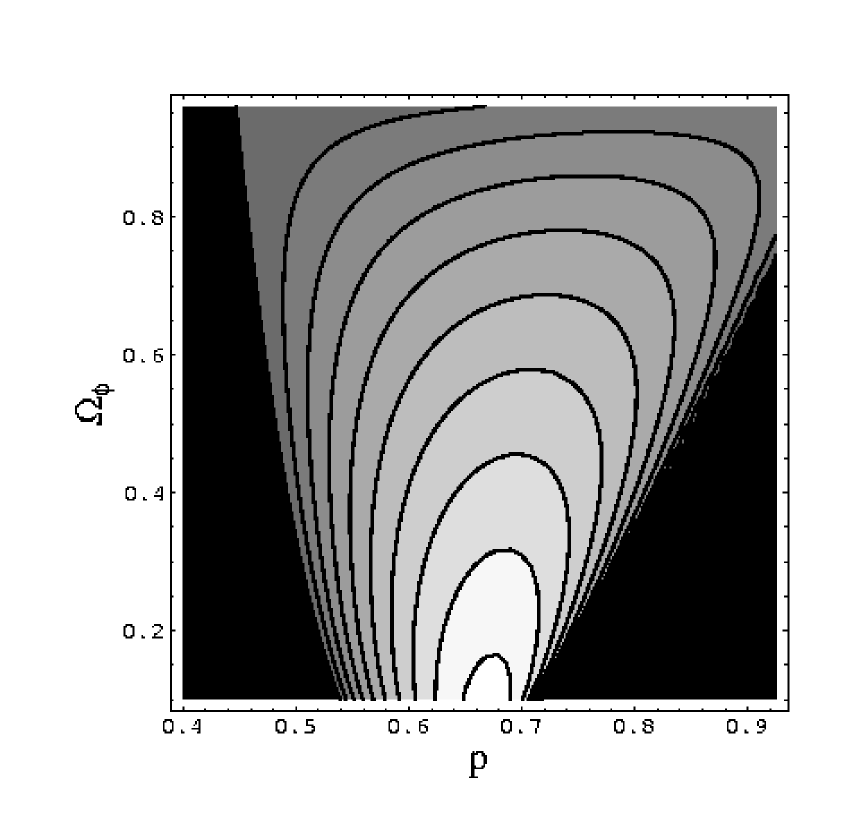
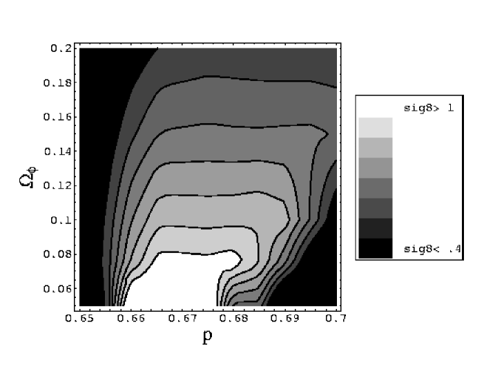
In Fig. 6 we report the power spectra normalized to COBE, compared to the data as compiled and corrected for redshift and non-linear distortions by Peacock & Dodds (1994). For a quantitative comparison, we plot in Fig. 7 the contour plot of , the number density variance in 8 /h spheres. The models with a value of larger than 0.5, as required by cluster abundance (White, Efstathiou & Frenk 1993, Viana & Liddle 1996, Girardi et al. 1998), have and at most a small deviations from . The suppression of with respect to COBE-normalized standard CDM is due both to the growth suppression in MDE and to the fact that now the COBE normalization includes the ISW effect.
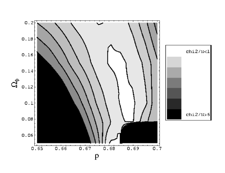
For as concerns the shape of the spectrum, the comparison with the galaxy data is uncertain due to biasing. Assuming a scale-independent bias between matter and galaxies, we can quantify the agreement with the data by evaluating the of the ratio between the theoretical and the galaxy spectrum, that is by evaluating
| (86) |
where are the average and variance of , neglecting cosmic variance. The contour plots of are in Fig. 8. They show, as anticipated, that the models with follow better the real data because are more bent at small scales. The best models among those studied here have for 15 degrees of freedom (16 real data, minus the average estimated from the data themselves). For instance the model with gives a very good fit, and has as required. Notice that we performed the fits without varying all the other cosmological parameters, which, at least in principle, can be determined by other observations.
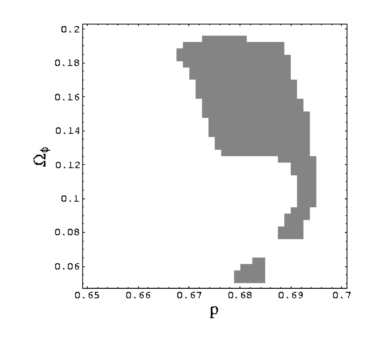
In Fig. 9 we summarize the constraints obtained in this Section, considering the models which have and . The cluster abundance normalization usually quoted for is , but this is calculated for standard models, so that conservatively a larger region has been adopted. Only a stripe around and appears to be viable, if the bias is indeed scale-independent. From Eq. (32) we deduce a limit
| (87) |
which, although still far from the limit 0.1 quoted in Wetterich (1995) from local measures, is global and applies even if the scalar field is not coupled to baryons, as proposed in Damour, Gibbons & Gundlach (1990). Future data will certainly tighten the constraint even further.
VII Conclusion
In this paper we discussed the perturbations of a coupled scalar field with exponential potential on the CMB and on the present large scale structure along an attractor solution. For as concerns the CMB, we found that the coupling induces a strong effect on the location and amplitude of the acoustic peaks, due to the variation of the scale factor expansion law. Future precision measures in the region have the potential of constraining the coupling to two orders of magnitudes better than at the present (see for instance the discussion in Chen & Kamionkowsky 1999).
We found that subhorizon perturbations are always more suppressed in MDE with respect to standard CDM, no matter what the parameters and are. Moreover, the suppression increases for far from the standard value. The amplitude at the present is between 0.5 and 1 only for , being smaller for larger , as already found in the uncoupled case by FJ. Adding the request to fit the galaxy power spectrum shape, the parametric space is reduced as in Fig. 9. A positive coupling has the advantage to warp the spectrum to a closer agreement with the data.
The background solution we adopted here is only one of the possible solutions. An equally interesting one is to consider a solution heading toward the inflationary attractor , but still short of it. This would provide closure density to a universe, and an acceleration as recently claimed, although at the price of sensibility to the initial conditions. Such a model will be investigated in a future work.
Acknowledgments
I am indebted to Carlo Baccigalupi, Francesca Perrotta and Michael Joyce for useful discussions on the topic.
REFERENCES
- [1] L. Amendola, astro-ph/9904120 (1999), to be published in Phys. Rev. D60
- [2] L. Amendola, C. Baccigalupi, R. Konoplich, F. Occhionero & S. Rubin, Phys. Rev. D54, 7199 (1996)
- [3] L. Amendola, M. Litterio & F. Occhionero, Int. J. Mod. Phys. A5, 3861 (1990)
- [4] L. Amendola, S. Gottloeber, J. Mucket, V. Muller, Ap.J., 451, 444 (1995)
- [5] L. Amendola, D. Bellisai & F. Occhionero, Phys. Rev. D47, 4267 (1993)
- [6] C. Baccigalupi, F. Perrotta & S. Matarrese, astro-ph/9906066 (1999)
- [7] R.R. Caldwell, R. Dave, & P.J. Steinhardt, Phys. Rev. Lett. 80, 1582 (1998)
- [8] R. Cen, N. Gnedin, L. Kofman, J.P. Ostriker, Ap.J., 399, L11 (1992)
- [9] X. Chen & M. Kamionkowski, astro-ph/9905368 (1999)
- [10] K. Coble, S. Dodelson, J. Frieman, Phys. Rev. D55, 1851 (1997)
- [11] E. J. Copeland, A.R. Liddle & D. Wands, Phys. Rev. D57, 4686 (1997)
- [12] T. Damour, G.W. Gibbons, C. Gundlach, Phys. Rev. Lett., 64, 123 (1990)
- [13] J. Ellis, S. Kalara, K.A. Olive & C. Wetterich, Phys. Lett. B228, 264 (1989)
- [14] P. G. Ferreira & M. Joyce, Phys. Rev. D58, 2350 (1998)
- [15] J. Frieman, C. T. Hill, A. Stebbins, & I. Waga, Phys. Rev. Lett. 75, 2077 (1995)
- [16] M. Girardi, S. Borgani, G. Giuricin, F. Mardirossian, M. Mezzetti, Ap.J., 506, 45 (1998)
- [17] S. Gottloeber, J. Mucket & A. Starobinsky, Ap.J., 434, 417 (1994)
- [18] F. Lucchin & S. Matarrese, Phys. Rev. D32, 1316 (1985)
- [19] C.P. Ma & E. Bertschinger, Ap.J. 455, 7 (1995)
- [20] J. Peacock & S. Dodds, MNRAS, 267, 1020 (1994)
- [21] S. Perlmutter et al. Nature 391, 51 (1998)
- [22] F. Perrotta & C. Baccigalupi, astro-ph/9811156, to be published in Phys. Rev. D59
- [23] B. Ratra, & P.J.E. Peebles, Phys. Rev. D37, 3406 (1988)
- [24] A. G. Riess et al. astro-ph/9805201 (1998)
- [25] S. Sarkar, Rep. Prog. Phys. 59, 1493 (1996)
- [26] U. Seljak & M. Zaldarriaga, Ap.J., 469, 437 (1996)
- [27] J.-P. Uzan, astro-ph/9903004, to be published in Phys. Rev. D59
- [28] P. Viana & A. Liddle, Phys. Rev. D57, 674 (1998)
- [29] P. Viana & A. Liddle, MNRAS 281, 323 (1996)
- [30] I. Waga & A. Miceli, astro-ph/9811460
- [31] C. Wetterich, Nucl. Phys. B252, 309 (1985)
- [32] C. Wetterich, Nucl. Phys. B302, 668 (1988)
- [33] C. Wetterich, A&A, 301, 321 (1995)
- [34] S.D.M. White, G. Efstathiou, C.S. Frenk, MNRAS 262, 1023 (1993)
- [35] I. Zlatev, L. Wang & P. J. Steinhardt, astro-ph/9807002 (1998)