Extended Quintessence
Abstract
We study Quintessence cosmologies in the context of scalar-tensor theories of gravity, where a scalar field , assumed to provide most of the cosmic energy density today, is non-minimally coupled to the Ricci curvature scalar . Such ‘Extended Quintessence’ cosmologies have the appealing feature that the same field causing the time (and space) variation of the cosmological constant is the source of a varying Newton’s constant à la Jordan-Brans-Dicke. We investigate here two classes of models, where the gravitational sector of the Lagrangian is with (Induced Gravity, IG) and (Non-Minimal Coupling, NMC). As a first application of this idea we consider a specific model, where the Quintessence field, , obeying the simplest inverse power potential, has today, in the context of the Cold Dark Matter scenario for structure formation in the Universe, with scale-invariant adiabatic initial perturbations. We find that, if for IG and for NMC ( is the present Quintessence value) our Quintessence field satisfies the existing solar system experimental constraints. Using linear perturbation theory we then obtain the polarization and temperature anisotropy spectra of the Cosmic Microwave Background (CMB) as well as the matter power-spectrum. The perturbation behavior possesses distinctive features, that we name ‘QR-effects’: the effective potential arising from the coupling with adds to the true scalar field potential, altering the cosmic equation of state and enhancing the Integrated Sachs-Wolfe effect. As a consequence, part of the CMB anisotropy level on COBE scales is due to the latter effect, and the cosmological perturbation amplitude on smaller scales, including the oscillating region of the CMB spectrum, has reduced power; this effect is evident on CMB polarization and temperature fluctuations, as well as on the matter power-spectrum today. Moreover, the acoustic peaks and the spectrum turnover are displaced to smaller scales, compared to ordinary Quintessence models, because of the faster growth of the Hubble length, which - for a fixed value today - delays the horizon crossing of scales larger than the horizon wavelength at matter-radiation equality and slightly decreases the amplitude of the acoustic oscillations. These features could be detected in the upcoming observations on CMB and large-scale structure.
I Introduction
Recently a lot of work focused on the cosmological role of a
minimally-coupled scalar field, considered as a ”Quintessence” (Q) component
which is supposed to provide the dominant contribution to the energy density
of the Universe today in the form of dynamical vacuum energy or ‘decaying
cosmological constant’ [1] -[5].
This work was motivated by the observational trend for an
accelerating Universe, as suggested by distance measurements to type Ia
Supernovae (see e.g. [6], [7]).
The main feature of such a vacuum energy component, that could
also allow to
distinguish it from a cosmological constant, is its time-dependence and
the wider range of possibilities for its equation of state compared to
the cosmological constant case.
In order not to violate the principle of general covariance,
such a time varying scalar field should also develop spatial
perturbations.
Noticeably, if one assumes that the Universe has critical density
as predicted by most inflationary models, this component could be the form
in which nearly two thirds of such a density resides.
The major success of the Quintessence models is their capability to
offer a valid alternative explanation of
the smallness of the present vacuum energy density
instead of the cosmological constant; indeed, we must have
GeV4 today, while
quantum field theories would predict a value for the cosmological constant
energy density which is larger by more than 100 orders of magnitude (for a
review, see for example [8],[9]).
On the other hand, in all the models considered up to now, the vacuum
energy associated to the Quintessence is dynamically evolving towards
zero driven by the evolution of the scalar field.
Furthermore, in the Quintessence scenarios one can select a subclass of
models, which admit ”tracking solutions” [10]: here a
given amount
of scalar field energy density today can be reached starting from a wide
set of initial conditions.
We are therefore encouraged to pursue the investigation of Quintessence
models.
The classical tests of gravity theories put severe constraints on the
scalar field term arising in the action; by far, the strongest constraint
being the Eötvös-Dicke experiment [11].
To avoid having to require a
coincidental similarity between different Yukawa couplings, one must
constrain to very small values any explicit coupling of the scalar field
to ordinary matter [4].
The possible coupling between a Quintessence field and light matter
has been explored in [12] and it is subject to restrictions
from the constraints on the time variation of the constants of
nature; a recent work explores several cosmological consequences
of a coupling between Quintessence and matter fields [13].
Moreover, a possible coupling between the scalar field,
modeling the Quintessence component, and the Ricci scalar
is not to be excluded in the context of generalized
Einstein gravity theories.
Due to the required flatness of its
potential to achieve slow-rolling, the coupling between
Quintessence field and other physical entities
gives rise to long-range () interactions;
in the case of coupling with the Ricci scalar, these long-range
interactions are of gravitational nature, giving rise to time variation
of the Newtonian constant, so that the
coupling parameter is constrained by solar system experiments
[14]. Recently,
some authors [15], [16] considered scalar-tensor theories of
gravity in the context of Quintessence models,
studying the existence and stability of cosmological scaling solutions.
Here we present the evolution of cosmological perturbations in some
subclass of these theories, where the scalar field coupled with
will be proposed as the Quintessence candidate, and we discuss its role
on CMB anisotropies and on structure formation in the Universe.
We name our model ‘Extended Quintessence’ (EQ), in analogy with
Extended Inflation models [17], where a Jordan-Brans-Dicke (JBD)
scalar field [18] was added to the action to solve the ‘graceful
exit’ problem of
‘Old Inflation’. Of course, the similarity
is not complete: in Extended Inflation a second scalar field -
the ‘Inflaton’, undergoing a first-order phase transition, was the actual
source of vacuum energy during inflation. Here, instead, we are supposing
that our non-minimally coupled scalar field has its own potential which
gives rise to a time (and space) varying cosmological constant term
dominating the present-day energy density of the Universe.
The first proposal of using a non-minimally coupled scalar field to
obtain a decaying cosmological constant dates back to 1983, when
Dolgov [19] suggested to exploit the effective negative energy term
contributed by the coupling of a massless scalar field
with the Ricci scalar
to drive the overall vacuum energy density to zero
asymptotically. The main problem with such a simple model is that the
interesting
dynamical range is achieved when the change in the effective Newton’s
constant strongly contradicts upper limits on solar system experiments
(see [9]).
Our model will differ from Dolgov’s idea in that
we will not assume that the non-minimal coupling term is the only cause of
time variation for the effective vacuum energy contribution.
This allows us to easily achieve consistency
with the solar system experimental limits on the coupling constants.
In this paper we present the background and perturbations equations
in the most general form and we consider their evolution for
Induced Gravity (IG) and Non-Minimally Coupled (NMC) scalar field models.
The Induced Gravity model was initially proposed by Zee in 1979
[20], as a theory for the gravitational interaction incorporating
the concept of spontaneous symmetry breaking; it was based on the observation
in gauge theories that dimensional coupling constants arising in a
low-energy effective theory can be expressed in terms of vacuum expectation
values of scalar fields.
This model was subsequently incorporated in models of
inflation with a slow-rolling scalar field [21];
in a modified form it was
the key ingredient of the Extended Inflation [17] class of models.
More recently, it has also been adopted in open inflation
models [22].
In [20], a scalar field coupled to gravity by a term proportional
to in the Lagrangian, is anchored by a symmetry-breaking
potential to a fixed value which eliminates the potential energy in
the present broken-symmetric phase of the world. We propose here a
different role for this scalar field, in the sense that we keep the same
coupling with the Ricci scalar as [20], but we allow for a larger
class of potentials than the Coleman-Weinberg one, also including
potentials that do not possess a minimum and can therefore contribute to
the present Quintessence energy density.
The second class of theories to which we apply our treatment is that of
non-minimal coupling of a scalar field to the Ricci curvature, described
extensively in curved space quantum field theory textbooks (e.g.
[23]).
The work is organized as follows: in Sec. II we present the relevant equations, defining the dynamical system for the background as well as for the perturbations in non-minimally coupled scalar field cosmologies; Sec. III is devoted to the definition of the IG and NMC models and to the analysis of the background evolution; Sec. IV contains and discusses the results of the numerical integration. Finally, Sec. V contains a brief summary of the results and some concluding remarks.
II Cosmological equations in scalar-tensor theories of gravity
Our purpose is to describe a class of scalar-tensor theories of gravity represented by the action
| (1) |
where is the Ricci scalar, is a constant needed to fix units
and is a classical
multicomponent-fluid Lagrangian including also minimally coupled scalar
fields, if any. We disregard any possible coupling of our scalar field
with ordinary matter, radiation and dark matter [24].
We assume a standard Friedman-Robertson-Walker (FRW) form for the
unperturbed background metric and we restrict ourselves to a spatially
flat universe.
We are using units where , but the convention concerning will be stated later, since it will depend on the choice of a
specific theory included in this general description. Instead, following
[26], we will choose the relation to
identify . Greek indices will be used for space-time
coordinates, latin ones will label spatial ones. We use the
signature .
By defining , the gravitational field equations derived by the action
(1) are
| (2) |
Here is the Einstein tensor, and all the other contributions have been absorbed in ; as noted in ([25],[26]), if one writes the gravitational field equation in this form, then can be treated as an effective stress-energy tensor, which allows to use the standard Einstein equations by simply replacing the fluid quantities with the effective ones. The background effective quantities following from the definition of are
| (3) |
where the overdot denotes differentiation with respect to the conformal time and .
The background FRW equations read
| (4) |
| (5) |
while the Klein-Gordon equation reads
| (6) |
Furthermore, the continuity equations for the individual fluid components are not directly affected by the changes in the gravitational field equation, and for the th component
| (7) |
In this background, the trace of (2) becomes
| (8) |
recalling that ; note that also appears in the right hand side of the equation, unless is of the form . An expression that will be useful in the following is that of the Ricci scalar,
| (9) |
Our treatment of the perturbations to this background follows (and
generalizes) a previous work [5], based on the formalism
developed in [27] to
describe the evolution of perturbations in the synchronous gauge.
A scalar-type metric perturbation in the synchronous gauge is
parameterized as
| (10) |
| (11) |
where denotes the trace of ; the fluid perturbations are described in terms of the variables , , and .
In terms of the effective fluid, the perturbed quantities can be written as
| (12) |
| (13) |
| (14) |
| (15) |
The perturbed Klein-Gordon equation reads
| (16) |
Note the presence of the Ricci curvature scalar in the term in the left hand side, as well as its perturbation in the right hand one.
All these ingredients have to be implemented in the perturbed Einstein equations
| (17) | |||||
| (18) | |||||
| (19) | |||||
| (20) |
This set of differential equations can be integrated once initial conditions on the metric and fluid perturbations are given; in this work we adopt adiabatic initial conditions (see [5]) for the various components and we perform the numerical integration of the system above for two specific classes of scalar-tensor theories, that will be defined in the next section.
The numerical integration has been performed by modifying the standard code CMBFAST [34]. The Q model case was introduced into the code in [5] where we investigated the perturbations behavior in these models. Here we provide a further extension to cover EQ models. As a main difference regarding the background evolution, the initial conditions for the Quintessence have to be searched by an iterative method that fixes the initial and values so that at the present time the Quintessence energy density has the required amplitude.
III Induced gravity and non-minimally coupled scalar field models
As we mentioned in the Introduction, two subclasses of non-minimally coupled scalar field theories have been considered [20], [21], [23]. Let us define them in the formalism of the previous Section.
Both these models can be obtained by setting
| (21) |
so that many of the formulas in the previous section simplify; also we take requiring that has the correct physical dimensions of . Note that all this fixes the link between the value of today and the Newtonian gravitational constant :
| (22) |
Also, this allows to define a time variation of the gravitational constant in non-minimally coupled theories,
| (23) |
(where the subscript indicates differentiation w.r.t. the cosmic time ) that is bounded by local laboratory and solar system experiments [28] to be
| (24) |
There is another independent experimental constraint coming from the effects induced on photons trajectories [29]. As well known, by making the transformation such that
| (25) |
the condition has to be imposed at the present time. It is easy to see that in our case this takes the form
| (26) |
where is the derivative of w.r.t. calculated at the present time. As we shall see, this constraint turns out to be the dominant one for our models.
Now let us proceed to the definition of the IG and NMC models.
In Induced Gravity (IG) models the gravitational constant is directly linked to the scalar field itself, as originally proposed in the context of the Brans-Dicke theory. We treat here this case by setting
| (27) |
where is the IG coupling constant In this case equations (22,24,26) become respectively
| (28) |
| (29) |
The minimally coupled case is recovered from IG models in the limit ; because of equation (29) this implies , and it can be quite easily verified that these conditions reduce all the equations written in the previous case to ordinary general relativity.
In non-minimally coupled (NMC) scalar field models the term multiplying the curvature scalar is made of two contributions: the dominant one, which is a constant, plus a term depending on ; minding the constraint on F at the present time, from equation (22), this can be written in the most general way as
| (30) |
Then, we choose in equation (30) as
| (31) |
where again is a coupling constant §§§Note that we define here the coupling constant with the opposite sign w.r.t. the standard notation for NMC models. and the constraints (24,26) become
| (32) |
Contrary to the IG case, we are now free to set , and the ordinary GR case is recovered by taking . Having no restrictions about this point, in our numerical integrations we fixed , the Planck mass (in natural units). We will only consider here for definiteness the case . The most general case, regarding the background evolution only, is discussed in [14].
Let us just mention here that one can always map this kind of scalar-tensor theories of gravity to canonical general relativity, by means of a conformal (Weyl) transformation, leading to the so-called Einstein frame (see, e.g. the recent review in [30]), where the gravity sector of the action takes the standard Einstein-Hilbert form. In the latter frame, the Quintessence field would be minimally coupled with gravity, but it would show explicit couplings with all the matter components. This mathematical technique is particularly useful if one is looking for scaling solutions [15]. We will not adopt this procedure here, but we will make all our calculations in the present physical frame, also called ‘Jordan frame’.
Let us elevate now to the role of Quintessence. This requires giving it a non-zero potential . Several potentials have been proposed for the Quintessence. In [3], the authors analyzed a cosine potential motivated by an ultra-light pseudo Nambu-Goldstone boson, while in other works, trying to build a phenomenological link to supersymmetry breaking models, inverse power potential have been considered [10],[31]. As pointed out in [32], inverse power potentials appear in supersymmetric QCD theories [33]. Here we take the simplest potential of the second class,
| (33) |
where the mass-scale is fixed by the level of energy contribution today from the Quintessence.
We are now ready to make some preliminary investigation of the background model. We require that the present value of is , with Cold Dark Matter at , three families of massless neutrinos, baryon content and Hubble constant Km/sec/Mpc; the initial kinetic energy of is not important since it is redshifted away during the evolution, so we can fix an equal amount of kinetic and potential energy at the initial time .
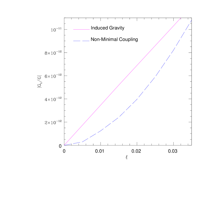
Let us introduce the next Section by fixing the compatibility of our models with the experimental constraints (24,26). A first version of these results, valid only for NMC models, can be found in [14].
First, we integrate equations (4,6) to compare with the experimental constraint of Eq.(24). The results are shown in Fig.1, where at the present time is shown as a function of . Both for NMC and IG, the limit roughly is
| (34) |
However, as we anticipated, the stronger constraint comes from Eq.(26); it is simple to see that in our models Eqs.(29,32) become
| (35) |
| (36) |
In the next section we will explore the effects on the cosmological perturbations spectra of EQ models, also considering values of beyond the above constraints, in order to better illustrate its effect on the cosmological equations. Then, we will discuss how future CMB experiments like MAP and Planck will be able to detect features of the present models within the range allowed from Eqs.(35,36).
IV QR-effects on cosmological perturbations
Here we present the results coming from the integration of the complete set of equations of Sec. II. The numerical integration of this set of equations has not been performed before, and we obtain several new and interesting effects concerning cosmologies with a coupling between Quintessence and the Ricci curvature scalar , that we name ‘QR-effects’; we discuss them in the following subsections.
Let us now set initial conditions for the perturbation equations, referring to [5] for an extensive treatment. We adopt isoenthropic (i.e. adiabatic) initial conditions; in the minimal coupling case they are quite simple: everything is initially zero except for the metric perturbation . It is easy to check that these conditions remain valid also in the present case. In fact, adiabaticity is imposed on each fluid separately, by requiring that the entropy perturbations is equal to zero initially for each pair of fluid components, including Quintessence [5]; these conditions do not depend on the coupling of a given component with .
As we anticipated, the scalar-tensor theories of gravity that we consider leave several characteristic imprints on cosmological perturbations spectra. Also, both IG and NMC models, although for different coupling constant ranges, show a remarkably similar behavior. For clearness, we shall treat first the features related to the background evolution and successively the genuine QR-effects on perturbations.
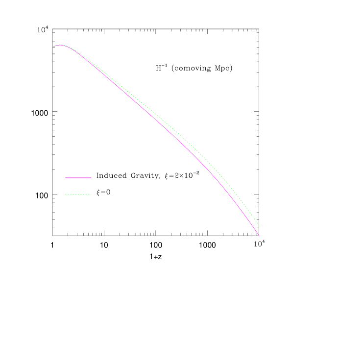
A QR-effects on the background: enhanced Hubble length growth and
Let us consider the Hubble length first. The integration of Eqs.(4,5) with the potential (33) shows that the time derivative of the Hubble length, , increases at non-zero redshifts compared with the ordinary Quintessence case, both for NMC and IG models. Therefore, fixing the Hubble length at present as we do, implies that in the past it was smaller than in minimally coupled models. This effect is clearly displayed by Fig.2, where the comoving Hubble length as a function of is shown (for simplicity we plot the IG case only, the NMC one being completely equivalent). This feature has been already noted in the context of pure Brans-Dicke theories [35]. The sharp change in the time dependence of at small redshifts is due to the Q-field, that dominates the cosmological evolution at later times.
The source of the enhanced Hubble length growth in our models is the last term in the Einstein equation (5); as we will show in a moment, this term is quite large and positive, being also responsible for most of the features that we shall see later concerning the cosmological perturbation spectra.
A related interesting point is that our model predicts a small change in which mimics a change in the number of massless neutrinos at the Nucleosynthesis epoch (see [36] for an extensive overview). At this time Quintessence is very subdominant and the cosmological evolution is governed by the equation
| (37) |
since in our models at any past time, the shift in the value of due the time variation of the gravitational constant in EQ models is given by:
| (38) |
As a function the shift of the number of relativistic species at Nucleosynthesis, the above quantity may be written as
| (39) |
Therefore, the shift predicted in our models is
| (40) |
It is worthwhile to note that for models satisfying Eq.(26), the predicted is at the level of , thus being well below the current experimental constraints from the Nucleosynthesis.
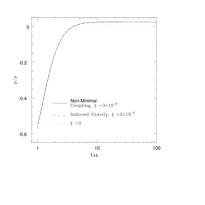
Let us consider now the effects of our scenario on the cosmological equation of state. The term appears also in the effective fluid pressure in Eq.(3), causing the following interesting feature in the behavior of the equation of state, shown in Fig.3. As it is evident, in the matter dominated era up to , when the Quintessence starts to dominate. Thereafter, the cosmic expansion starts to accelerate because of the vacuum energy stored in the Quintessence potential. Thus we have the apparent paradox that in the matter dominated era the total pressure is non-zero and positive: this is not surprising since it can be brought back to the dynamics of the scalar field itself in scalar-tensor theories of gravity. Corresponding to its positive value in the matter dominated era, the equation of state at present, when Quintessence dominates, is slightly above its value for Q models. In other words, we found that the Quintessence contribution to the equation of state in our models, , does not change significantly in our case with respect to Q models; we found indeed
| (41) |
for all the cases considered. This is well within the range of values for which the Quintessence is mimicking a cosmological constant [37], [7].
Let us now come to the effect. This interesting and very peculiar occurrence can be understood by looking at the behavior of the various components of the energy density in Eq.(4) and is obviously connected with the effect on the equation of state just described. After dividing both members by , the Friedmann equation takes the form
| (42) |
where it must be noted that is actually made of three terms, namely
| (43) |
While and are the generalization of the kinetic and potential energy densities in scalar-tensor theories, the really new component is
| (44) |
which, as we already noted, is negative if . Its amplitude is fixed essentially by the dynamics of the scalar field; as we anticipated, this term turns out to be important for the background evolution. The reason is the following. In all the cases considered, the scalar field evolution is slow, so that and the time variation of the potential in the Klein-Gordon equation can be neglected. Let us consider the radiation dominated era for simplicity: , where is a constant. Therefore, it is immediate to check that the approximate solution of the Klein Gordon equation is
| (45) |
In the ideal case where the scalar field evolves for a large time so that only the term proportional to is important, we see that ; in this case the term in Eq.(44) would be of order unity. In the real case these arguments are weakened since the scalar field does not have a perfect slow-rolling dynamics, and it does not evolve enough to become much larger than its initial value; nevertheless this qualitatively explains why we found for models satisfying the constraints (26), and for a time interval roughly covering all the post-equality cosmological history.
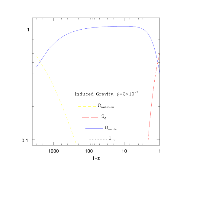
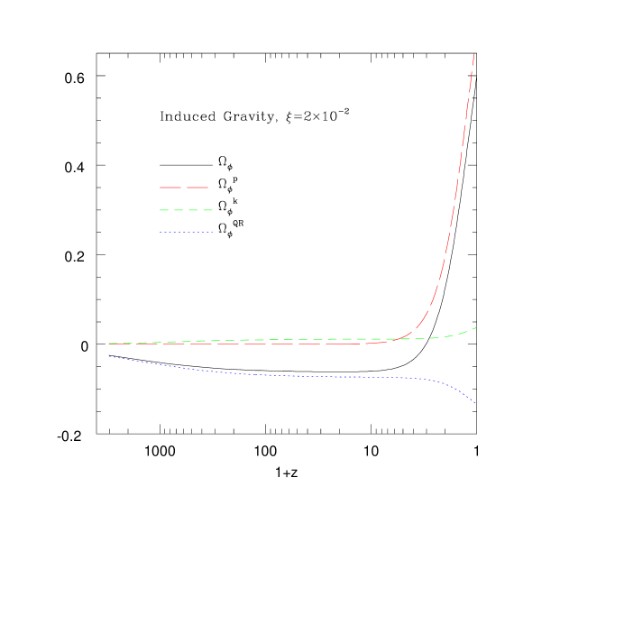
Fig.4 shows the various contributions to the cosmic density parameters as a function of redshift. The matter radiation equality epoch is clearly visible, as well as the matter dominated era, and, finally, the Quintessence dominated era at very small redshifts. Also, the sum (identically equal to 1) is shown, and it is immediately seen that in the matter dominated era one has
| (46) |
As we already anticipated this is only an apparent paradox, because of the presence of the negative energy component in the Einstein equation (4), explicit in Eq.(44). Figure 5 shows the various contributions to the Quintessence energy density. As it can be seen, for the chosen value of the coupling constant , reaches values of a few percent and is responsible for the condition (46).
This completes a rapid survey of the features regarding the cosmological background evolution; some of them have a relevant influence on the perturbation behavior, that is the subject of the next subsection.
B QR-effects on the CMB: Integrated Sachs-Wolfe effect, horizon crossing delay and reduced acoustic peaks
The phenomenology of CMB anisotropies in EQ models is rich and possesses distinctive features.
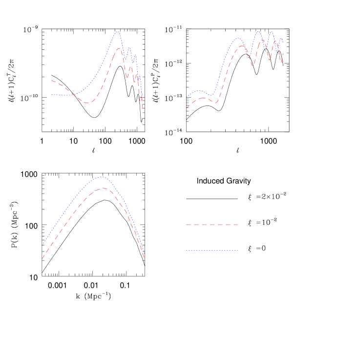
In the top left panel of Fig.6, the effect of increasing on the power spectrum of COBE-normalized CMB anisotropies is shown. Note that we plotted cases also exceeding the limit (26), to make clearer the perturbations behavior in EQ scenarios. The rise of makes substantially three effects: the low ’s region is enhanced, the oscillating one attenuated, and the location of the peaks shifted to higher multipoles. Let us now explain these effects. The first one is due to the integrated Sachs-Wolfe effect, arising from the change from matter to Quintessence dominated era occurred at low redshifts. This occurs also in ordinary Q models, but in EQ this effect is enhanced. Indeed, in ordinary Q models the dynamics of is governed by its potential; in the present model, one more independent dynamical source is the coupling between the Q-field and the Ricci curvature . As it can be easily understood by the Lagrangian in equation (1), the scalar field evolves as dictated by the effective potential
| (47) |
As it is clear from equation (9), is positive in the matter dominated era, (). Thus, from (47), after differentiating with respect to , both the forces coming from are negative, pushing together the field towards increasing values. In conclusion, the dynamics of is boosted by together with its potential . As a consequence, part of the COBE normalization at is due to the Integrated Sachs-Wolfe effect; thus the actual amplitude of the underlying scale-invariant perturbation spectrum gets reduced. This is the main reason why the oscillating part of the spectrum, both for polarization and temperature, is below the corresponding one in Q-models.
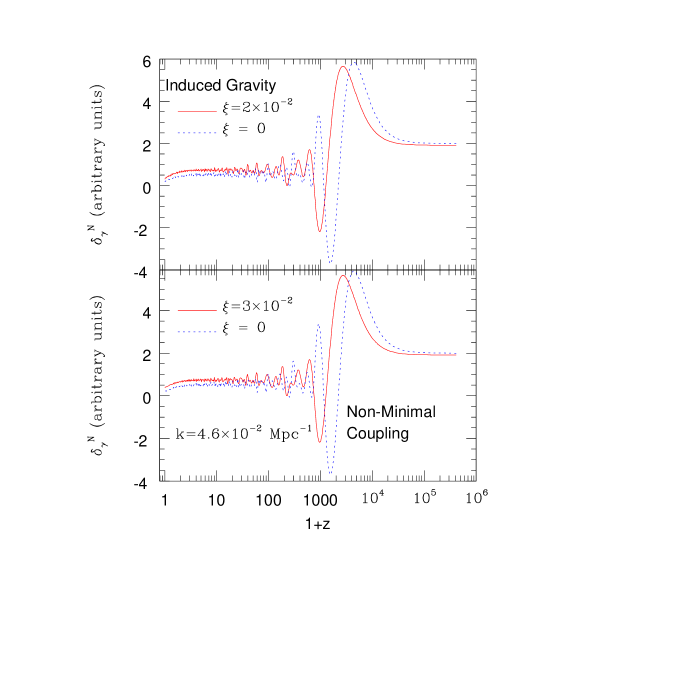
There is however another effect that slightly reduces the amplitude of the acoustic oscillations. We have seen in Fig.2 that the Hubble length was smaller in the past in EQ than in Q models. This has the immediate consequence that the horizon crossing of a given cosmological scale is delayed. This is manifest in Fig.9, where we have plotted the photon density perturbation in the Newtonian gauge ; we choose this quantity since it is simply 4 times the dominant term of the CMB temperature fluctuations [38]. Its expression in terms of the quantities in the synchronous gauge is
| (48) |
The scale shown in Fig.9 is chosen so that it reenters the horizon roughly between matter-radiation equality and decoupling. Both in the IG and NMC cases, it is evident that the oscillations start later than in ordinary Q models. As well known, the amplitude of the acoustic oscillations slightly decreases if the matter content of the universe at decoupling is increased [5, 3].
Finally, note how the location of the acoustic peaks in term of the multipole at which the oscillation occurs, is shifted to the right. Again, the reason is the time dependence of the Hubble length, which at decoupling, subtended a smaller angle on the sky. It is straightforward to check that the ratio of the peak multipoles in Fig.6 coincides numerically with the the ratio of the values of the Hubble lengths at decoupling in Fig.2 in EQ and Q models.
These considerations do not change at all for NMC models. Really, IG and NMC models present, for different values of , remarkably similar features, yielding a genuine signature of scalar tensor-theories in the cosmological perturbations spectra.
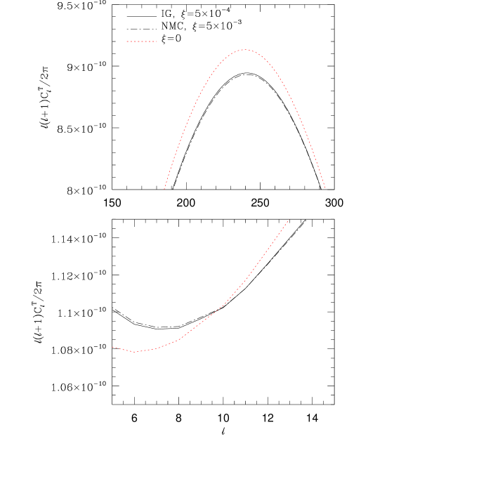
Let us consider now realistic cases respecting the constraints from Eq.(26). Figs.7,8 show the temperature perturbation spectra for NMC and IG cases with the indicated coupling constants. The effects described previously are evident particularly in Fig.8, where the changes in the first acoustic peak (top) and in the power at low ’s (bottom) have been zoomed; also, the slight difference between IG and NMC models is visible. We notice that features of this amplitude in the CMB spectra, induced by models satisfying the existing constraints from Eqs.(24,26) are detectable by the future generation of CMB experiments; in particular, MAP and Planck will bring the accuracy on the CMB power at percent level up to [40].
C QR-effects on matter perturbations: power-spectrum decrease and peak shift
After decoupling, the different models considered in Fig.6 evolve until the present, when we snapshot the matter power-spectrum in the bottom left panel.
Soon after their introduction, Q-models were considered more appealing than those involving a cosmological constant term because of their capability to shift the power-spectrum toward larger scales without increasing its overall amplitude, which would have required an antibias mechanism. We find here that this effect is enhanced if a QR-coupling exists. This is evident in both the bottom right panel in Fig.6. The spectra are COBE-normalized as it is evident in the top panel. For increasing , the spectra loose power. The reason of this behavior is that the CMB spectra include different effects together with the true perturbation amplitude; on the large scales measured by COBE, the matter perturbations add with the large Integrated Sachs-Wolfe effect; the greater is , the stronger being the Integrated Sachs-Wolfe effect, the weaker the true perturbations amplitude, as we pointed out in the previous subsection. This causes the power-spectrum decrease that is well visible in the figure.
The other effect is the slight shift of the location of the peaks toward larger wavenumbers. Again, this is due to the time dependence of ; since it is smaller in extended Quintessence models than in ordinary Quintessence ones, the horizon crossing is delayed for all the cosmological scales, for the given value of .
These are the most prominent features concerning the power-spectrum. In principle however, there are terms in the cosmological perturbation equations that could make some relevant effects. We search them as terms that do not multiply fluctuations in the scalar field, since the latter are negligible from the point of view of structure formation [5]. Looking indeed at Eq.(15), the last term in the r.h.s. could play some role: it is the shear perturbation associated with the Quintessence and it should be noted that it is not present in ordinary Q models. Looking at Eq.(20), it is immediate to verify that this term produces a sort of excess friction in the dynamics of the quantity in addition to the cosmological Hubble drag term in the l.h.s.: we define it as
| (49) |
Its relevance compared to has been already discussed when we dealt with the quantity of Eq.(44). As it is evident in Fig.10, is not so important during the evolution since it is only a few percent of the Hubble drag during all the evolution. Although clearly plays the role of a sort of integrated shear effect, it is less important than those described at the beginning of this subsection.
These effects change the matter power-spectrum today in a way that we will better explore in a future work. Here we make a first comparison with the known expectations concerning the spectrum normalization at Mpc, . Recently the cluster abundance in Q models has been analyzed [39]. An empirical formula for in these models has been found as
| (50) |
where
| (51) |
is the spectral index (1 in our scale-invariant case), is the present Hubble constant in units of 100km sMpc-1 and the matter energy amount today. The existing experimental constraints (see [39]) may be expressed as follows:
| (52) |
Our scenario is not significantly constrained by Eq.(52). For the models shown in Fig.6, we found
| (53) | |||||
| (54) | |||||
| (55) |
It is easy to verify that the constraint in Eq.(52) is satisfied for ; the same limit for NMC models is . It is remarkable however that future experiments will be able to provide much more accurate measurements of the matter power spectrum [41].
V Summary and concluding remarks
Our work is based on the possibility that the cosmological vacuum energy that seems required to explain the data from high-redshift type Ia Supernovae resides in the potential energy of a slowly rolling scalar field or Quintessence. We considered models in which the Quintessence scalar field is non-minimally coupled with the Ricci curvature scalar , that we named Extended Quintessence.
With this aim, and based on a technique obtained in some recent works [25, 26, 5], we integrated the full linear cosmological perturbation equations for generalized Einstein gravity theories. In this framework we investigated the effects produced by two distinct Extended Quintessence models, in which the gravitational part of the Lagrangian is
| (56) |
| (57) |
indicating the Q-value today.
Quintessence models are characterized by a potential energy that is comparable to the matter energy density today. We choose the simplest inverse power potential
| (58) |
with the constant fixed by requiring that the Quintessence energy density today yields .
The first check we made by integrating our equations, was whether our results are compatible with the bounds from the solar system experiments: we found that these constraints are satisfied if , for IG, and , for NMC models. We went then to a more detailed analysis of the effects on the power-spectra obtained, that we named QR-effects. We found several features that could help in discriminating these models from ordinary Quintessence.
In particular, the Integrated Sachs-Wolfe effect, caused by the time variation of the gravitational potential between last scattering and the present time, which is already active in ordinary Q-models, is now enhanced. This can be understood by considering the Klein-Gordon equation governing the time evolution of . It is easily seen that the coupling with induces a new source of effective potential energy; the latter is ineffective in the radiation dominated era, when , but becomes important during matter and scalar field dominance, when it originates the effective potential
| (59) |
It is therefore immediate to realize that the force in the Klein Gordon equation simply adds to the one coming from the true potential from (58), having the same sign and therefore enhancing the Integrated Sachs-Wolfe effect. As a consequence, part of the COBE normalization is now due to the latter effect and the cosmological perturbation amplitude, including also the oscillating region of the CMB spectrum, is reduced; this is evident in the CMB polarization and temperature patterns, as well as in the matter power-spectrum today. Moreover, the acoustic peaks and the power-spectrum turnover are displaced to smaller scales; the reason being that the Hubble length grows more rapidly in these theories than in ordinary Q-models, delaying - for a fixed value of - the horizon crossing of any scale larger than the Hubble radius at the matter-radiation equality, and slightly decreasing the amplitude of the acoustic oscillations.
Another independent QR-effect comes from the change of the fluid shear arising in generalized Einstein theories. From the Einstein equations it turns out that the new terms in induce an additional friction to the growth of the gauge-invariant gravitational potential , besides that due to the Hubble drag. This makes the growth of weaker, and, since in adiabatic models the acoustic oscillations are essentially driven by this quantity, this results in a reduced amplitude for the acoustic peaks.
For what concerns large-scale structure formation, we also considered the effect of the extra term in the fluid shear arising from the QR-coupling. It produces a sort of friction in the dynamics of the metric perturbations, in addition to the genuine cosmological friction. Although interesting, we found that this effect is negligible compared to the effect due to the Integrated Sachs-Wolfe effect that changes the normalization to COBE data.
It is also remarkable that similar features occur both in IG and NMC models, suggesting the existence of an extended Quintessence phenomenology that is the signature of a large class of scalar-tensor theories in the cosmological perturbations.
This is a brief summary of the results we obtained in this class of Extended Quintessence models. Of course, this work does not answer all the questions nor it explores all the aspects, but the results we obtained show distinctive and promising features at the point that we believe it should be seriously taken into account, especially in favor of the hints on the existence of scalar fields and on their possible couplings with coming from fundamental theories. An important problem to face is which effects are caused by the fact that we require that the field coupled with is a Quintessence, and which instead come from the scalar-tensor theories themselves. The enhanced Integrated Sachs-Wolfe effect appears to be mostly determined by the extra effective potential coming from the non-minimal coupling; on the contrary, the effects at decoupling appear to be caused mostly by the true scalar field potential, since at that time the Ricci scalar is much smaller than it is now. However, all these considerations, together for example with the exploration of other scalar field potentials and more general gravitational sectors in the Lagrangian, would deserve a separate work.
ACKNOWLEDGMENTS
We warmly thank Luca Amendola, Robert Caldwell and Karsten Jedamzik for precious comments and useful discussions.
While completing this paper a preprint by Chen and Kamionkowski [42] has appeared in which the CMB temperature and polarization patterns produced by a pure JBD field in a standard Cold Dark Matter cosmology have been considered. Although there is no overlap with our Quintessence field, it is worthwhile to note that, for what concerns the acoustic peak locations, their results show a similar dependence on the parameter.


REFERENCES
- [1] P.J. Peebles, B. Ratra, Astrophys. J. 352, L17 (1988); R.R. Caldwell, R. Dave, P.J. Steinhardt, Phys. Rev. Lett. 80, 1582 (1998).
- [2] P.G. Ferreira, M. Joyce , Phys. Rev. D 58 023503 (1998); P.T.P. Viana, A.R. Liddle, Phys. Rev. D57, 674 (1998).
- [3] K. Coble, S. Dodelson, J. Friemann, Phys. Rev. D 55, 1851 (1997).
- [4] B. Ratra, P.J. Peebles, Phys. Rev. D 37, 3406 (1988).
- [5] F. Perrotta, C. Baccigalupi, Phys. Rev. D 59, 123508 (1999).
- [6] S. Perlmutter et al., Nature 391, 51 (1998); A.G. Riess et al., Astron. J. 116, 1009 (1998).
- [7] P.M. Garnavich et al., ApJ in press, preprint astro-ph/9806396.
- [8] A.D. Dolgov, Lecture presented at the 4th Colloque Cosmologie, Paris (1997).
- [9] V. Sahni, A. Starobinski, preprint astro-ph/9904398 (1999).
- [10] P.J. Steinhardt, L. Wang, I. Zlatev, Phys. Rev. D 59, 123504 (1999); I. Zlatev, L. Wang, P.J. Steinhardt, Phys. Rev. Lett. 82, 896 (1999); A.R. Liddle, R.J. Scherrer, Phys. Rev. D 59, 023509 (1999).
- [11] P.G. Roll, R. Krotkov, R.H. Dicke, Ann. Phys. (N.Y.) 26, 442 (1964).
- [12] S.M. Carroll, Phys. Rev. Lett. 81, 15, 3097 (1998).
- [13] L. Amendola, preprint astro-ph/9908023 (1999).
- [14] T. Chiba, to appear in Phys. Rev. D, preprint gr-qc/9903094 (1999).
- [15] L. Amendola, Phys.Rev. D60 043501 (1999), astro-ph/9904120.
- [16] J.P. Uzan, Phys. Rev. D 59, 123510 (1999).
- [17] D. La, P.J. Steinhardt, Phys. Rev. Lett. 62, 376 (1989); F.S. Accetta, J.J. Trester, Phys. Rev. D 39, 2854 (1989); E.J. Weinberg, Phys. Rev. D 40, 3950 (1989).
- [18] P. Jordan, Z. Phys. 157, 112 (1959); C. Brans, R.H. Dicke, Phys. Rev. 124, 925 (1959).
- [19] A.D. Dolgov, In The Very Early Universe, eds. G.W. Gibbons, S.W. Hawking, S.T.C. Siklos, Cambridge University Press, Cambridge, p. 449 (1983).
- [20] F. Zee, Phys. Rev. Lett. 42, 417 (1979).
- [21] B.J. Spokoiny, Phys. Lett. B 147, 39 (1984); F.S. Accetta, D.J. Zoller, M.S. Turner, Phys. Rev. D 31, 3064 (1985); M.D. Pollock, Phys. Lett. B 156, 301 (1985); F. Lucchin, S. Matarrese, M.D. Pollock, Phys. Lett. B 167, 163 (1986).
- [22] J. Garcia-Bellido, Phys. Rev. D 55, 4603 (1997).
- [23] N.D. Birrel, P.C. Davies, Quantum Fields in Curved Spaces, Cambridge Univ. Press, Cambridge (1982).
- [24] T. Damour, G.W. Gibbons, C. Gundlach, Phys. Rev. Lett. 64, 123 (1990); G. Piccinelli, F. Lucchin, S. Matarrese, Phys. Lett. B 277, 58 (1992).
- [25] J.C. Hwang, ApJ 375, 443 (1991); J.C. Hwang, Phys. Rev. D 53, 762 (1996).
- [26] J.C. Hwang, Class. Quantum Grav. 7, 1613 (1990).
- [27] C.P. Ma, E. Bertschinger, ApJ 455, 7 (1995).
- [28] G.T. Gillies, Rep. Prog. Phys. 60, 151 (1997).
- [29] C.M. Will, Phys. Rep. 113, 345 (1984); T. Damour, to appear in Nucl. Phys. B (Proc. Suppl.) 1999; T. Damour, Eur. Phys. J. C3, 113 (1998); T. Damour, in Les Arcs 1990, Proceedings,”New and exotic phenomena ’90”, 285 (1990); R.D. Reasenberg et al., ApJ 234, L219 (1979).
- [30] V. Faraoni, E. Gunzig, P. Nardone, Fund. Cosm. Phys., in press, preprint gr-qc/9811047
- [31] J. Ellis et al., Phys. Lett. B 134, 429 (1984); E. Witten, Phys. Lett. B 155, 151 (1985); H. Nishino, E. Sezgin, Phys. Lett. B 144, 187 (1984).
- [32] P. Binétruy, preprint hep-ph/9810553.
- [33] T.R. Taylor, G. Veneziano, S. Yankielowicz, Nucl. Phys. B 218, 493 (1983); I. Affleck, M. Dine, N. Seiberg, Phys. Rev. Lett. 51, 1026 (1983), Nucl. Phys. B 241, 493 (1984); A. Masiero, M. Pietroni, F. Rosati, preprint hep-ph/9905346.
- [34] U. Seljak, M. Zaldarriaga, ApJ 469, 437 (1996).
- [35] A.R. Liddle, A. Mazumdar & J.D. Barrow, preprint SUSSEX-AST 98/2-2, astro-ph/9802133 (1998)
- [36] S. Sarkar, Rep. Prog. Phys. 59, 1493 (1996).
- [37] G. Efstathiou, preprint astro-ph/9904356.
- [38] W. Hu, U. Seljak, M. White, M. Zaldarriaga, Phys. Rev. D 57, 3290 (1998).
- [39] L. Wang, P.J. Steinhardt, ApJ 508, 483 (1998).
- [40] MAP home page: http://map.gsfc.nasa.gov/ ; Planck Surveyor home page: http://astro.estec.esa.nl/SA-general/Projects/Planck/
- [41] SDSS home page: http://www.sdss.org/ ; 2dF home page: http://msowww.anu.edu.au/ colless/2dF/
- [42] X. Chen, M. Kamionkowski, preprint astro-ph/9905368.