Measuring angular diameters of extended sources
I. Theory

Abstract

When measuring diameters of partially resolved sources like planetary nebulae, H ii regions or galaxies, often a technique called gaussian deconvolution is used. This technique yields a gaussian diameter which subsequently has to be multiplied with a conversion factor to obtain the true angular diameter of the source. This conversion factor is a function of the Full Width at Half Maximum (fwhm) of the beam (in the case of radio observations) or the point spread function (in the case of optical observations). It also depends on the intrinsic surface brightness distribution of the source.

In this paper the theory behind this technique will be studied. This study will be restricted to circularly symmetric geometries and beams. First an implicit equation will be derived, from which the conversion factor for a given surface brightness distribution and beam size can be solved. Explicit expressions for the conversion factor will be derived from this equation which are valid in cases where the beam size is larger than the intrinsic size of the source. A more detailed discussion will be given for two simple geometries: a circular constant surface brightness disk and a spherical constant emissivity shell with arbitrary inner radius. The theory is subsequently used to construct a new technique for determining the fwhm of an arbitrary observed surface brightness distribution.

Usually the fwhm of the source and beam are measured using gaussian fits, but second moments can also be used. The alternative use of second moments in this context is studied here for the first time and it is found that in this case the conversion factor has a different value which is independent of the beam size. In the limit for infinitely large beam sizes, the values of the conversion factors for both techniques are equal.

The application of the theory discussed in this paper to actual observations will be discussed in a forthcoming paper. This will include a comparison between optical and radio observations.

1 Introduction

The accurate measurement of angular diameters is a long standing problem. This problem is pertinent to the study of planetary nebulae, H ii regions, galaxies and other extended sources. Nevertheless, only few papers dedicated to this problem can be found in the literature: Mezger & Henderson [1967], Panagia & Walmsley [1978], Bedding & Zijlstra [1994], Schneider & Buckley [1996], and Wellman et al. [1997].

Several methods are in general use to determine angular diameters. One method determines the angular diameter of the source, based on the Full Width at Half Maximum (fwhm) of a two-dimensional gaussian fitted to the observed surface brightness distribution (also called profile in this paper) in a least-squares sense. This method is usually called gaussian deconvolution and will be explained in more detail below. The second method is basically identical to the first, except that it determines the fwhm using the second moment of the profile instead of a gaussian fit. To discriminate it from the first method, it will be called second moment deconvolution. Both methods have the disadvantage that they yield a result that has no well-defined physical meaning. Hence, a conversion factor is needed to translate the result into something meaningful. In nebular research this usually is the Strömgren radius. This conversion factor depends on the method being used, the intrinsic surface brightness profile of the source and the resolution of the observation.

The theory to determine the conversion factor is derived in this paper in several stages. First, in Section 2 some basic assumptions and definitions will be given. Next, in Section 3 the full analytical theory for gaussian deconvolution will be given. In Section 4 this theory will be used to construct an alternative algorithm to determine the fwhm of an observed surface brightness distribution. In Section 5 the theory will be given for second moment deconvolution. In Section 6 the main conclusions will be presented. In Appendix A some additional proofs will be presented and finally in Appendix B the most important symbols that have been used will be defined. The appendices are only available in electronic form.

2 Assumptions and definitions

The methods discussed in this article can be applied to observations at any wavelength. More in particular, they are valid for optical, infrared and radio observations. The resolution of these observations is usually characterized by the size of the beam profile for radio data or by the size of the point spread function for optical and infrared data. Throughout the paper the term ‘beam’ will be used and it will be implicitly understood that it can also mean ‘point spread function’ where appropriate. It will be assumed that the beam can be approximated by a gaussian. In this paper the intrinsic surface brightness profile will be defined as the profile that would be observed with a perfect instrument (i.e. an instrument with infinite resolving power). For simplicity it will be assumed throughout this paper that both the surface brightness distribution of the nebula and the beam are circularly symmetric. This is a rather severe restriction; nebulae rarely are circular, and also for radio observations the beam usually is elliptical. However, this simplified case already yields interesting results which can be applied to actual data.

As was already remarked, a conversion factor is needed to translate the fwhm diameter yielded by the gaussian or second moment deconvolution method into a Strömgren diameter. In this paper the Strömgren radius of the nebula will be denoted by $r_{\rm s}$. In the rest of this paper it will be assumed that the true diameter of the nebula is $\Theta_{\rm d}=2r_{\rm s}$. The measured fwhm of the nebula will be denoted by $\Phi$ and the fwhm of the beam by $\Phi_{\rm b}$. Throughout the paper the deconvolved fwhm diameter $\Phi_{\rm d}$ will be used, which is defined by

$$\Phi_{\rm d}=\sqrt{\Phi^{2}-\Phi_{\rm b}^{2}}.$$ (1)

This quantity is also commonly called the gaussian diameter. It should not be confused with the fwhm of the deconvolved or intrinsic profile, which in general will be different. The conversion factor to obtain the true angular diameter from the deconvolved fwhm can now be defined as

$$\Theta_{\rm d}=\gamma\Phi_{\rm d}\hskip 8.53581pt\Rightarrow\hskip 8.53581pt\gamma=\Theta_{\rm d}/\Phi_{\rm d}=2r_{\rm s}/\Phi_{\rm d}.$$ (2)

This conversion factor is a function of the resolution of the observation, or to be more precise, of the ratio of the observed source diameter and the beam size. Hence an independent parameter $\beta$ is chosen, which is defined as

$$\beta=\Phi_{\rm d}/\Phi_{\rm b}.$$ (3)

In the following sections more details will be given of the techniques that have been used to calculate the conversion factors, both for the gaussian and the second moment deconvolution method.

3 Determining diameters using gaussian fits

In this section the conversion factor will be studied for the case where the fwhm of the observed surface brightness profile is determined using gaussian fits. An implicit equation will be derived from which the value of $\gamma(\beta)$ can be solved for arbitrary $\beta$. This equation will also be used to derive the first terms of a Taylor series expansion of $\gamma(\beta)$ near $\beta=0$. This implicit equation is derived in three stages. First it will be shown how to derive the width of a gaussian fitted to an arbitrary profile in Section 3.1. Next an expression for a surface brightness profile convolved with a gaussian of arbitrary size will be derived in Section 3.2. Finally in Section 3.3 these results will be combined to determine the conversion factor. In this process various lemma’s will be used which can be found in Appendix A.

• in the remainder of this paper all functions are implicitly assumed to be circularly symmetric.

• in the remainder of this paper constraints have to be imposed on the surface brightness profile $f(r)$. When $c_{n}$ is defined as

  $$c_{n}=2\pi\!\intop_{0}^{\infty}f(r)r^{n+1}\mbox{\rm d}r,$$ (4)

  the following constraint can be formulated:

  $$\hbox{(1)}\hskip 14.22636pt0\leq f(r)\leq F\hskip 8.53581pt\hbox{for all }r\in[\,0,\infty),\hskip 8.53581pt\hbox{such that $c_{0}$ exists and }c_{0}>0.$$

  This condition is sufficient for the theory derived in Section 3.1. For the theory in Section 3.2 (up to Eq. 21) an additional constraint has to be imposed

  $$\hbox{(2a)}\hskip 11.38109ptc_{2n}\hbox{ exists for all }n\in{\mathbb{N}}_{0},\hskip 8.53581pt\hbox{with }c_{n}^{1/n}=o(n)\,(n\rightarrow\infty).$$

  It should be noted that the fact that $c_{n}$ exists automatically implies that all $c_{i}$ exist with $i\leq n$, as is shown in Lemma A. In the remainder of Section 3.2 and all subsequent sections, this constraint needs to be restricted to

  $$\hbox{(2b)}\hskip 11.38109ptc_{2n}\hbox{ exists for all }n\in{\mathbb{N}}_{0},\hskip 8.53581pt\hbox{with }c_{n}^{1/n}=o(n^{\frac{1}{2}})\,(n\rightarrow\infty).$$

  It is also worth noting that all profiles which fulfill the following condition

  $$\hbox{(2c)}\hskip 11.38109ptf(r)=0\hskip 8.53581pt\hbox{for all }r>R_{o},$$

  (where $R_{o}$ is some arbitrary outer radius) and which additionally fulfill condition (1), automatically fulfill condition (2b). This is proven in Lemma A. Since for all observational data conditions (1) and (2c) are automatically fulfilled, the theory presented in this paper is valid for all observed profiles. This neglects the fact that noise might cause some pixels to have negative flux values. In general this poses no problem however, as will be discussed in a forthcoming paper (van Hoof 1999). One should also note that for a perfect gaussian, condition (2b) is not fulfilled.

• in the remainder of this paper it is assumed that $r_{\rm s}=1$.

3.1 Fitting a gaussian to a surface brightness profile

In this section the formulae to approximate a surface brightness profile $f(r)$ with a two dimensional gaussian in a least-squares sense will be derived. The gaussian will be written as

$$g(r;a,p)=a\,\mbox{\rm e}^{-pr^{2}}\hskip 8.53581pt\hbox{with}\ a>0,\ p>0.$$

In order to determine a least squares fit to the surface brightness profile, the integral over the quadratic residuals $\chi^{2}$ needs to be minimized. Hence the following two equations need to be solved:

$$\frac{\partial\chi^{2}}{\partial p}=\frac{\partial}{\partial p}\intop_{0}^{2\pi}\intop_{0}^{\infty}\left[\,f(r)-g(r;a,p)\,\right]^{2}r\mbox{\rm d}r\mbox{\rm d}\varphi=0,$$ (5)

and

$$\frac{\partial\chi^{2}}{\partial a}=\frac{\partial}{\partial a}\intop_{0}^{2\pi}\intop_{0}^{\infty}\left[\,f(r)-g(r;a,p)\,\right]^{2}r\mbox{\rm d}r\mbox{\rm d}\varphi=0.$$ (6)

Eq. (5) will be evaluated first. After integration over $\varphi$ and reversal of the order of differentiation and integration one gets

$$-4\pi\!\intop_{0}^{\infty}\left[\,f(r)-g(r;a,p)\,\right]\frac{\partial g(r;a,p)}{\partial p}r\mbox{\rm d}r=0.$$

One can easily prove that this is allowed using Lemma A and A, provided condition (1) is fulfilled. Since

$$\frac{\partial g(r;a,p)}{\partial p}=-ar^{2}\mbox{\rm e}^{-pr^{2}}$$

one finds, after division by the constants,

$$\intop_{0}^{\infty}\left[\,f(r)-a\mbox{\rm e}^{-pr^{2}}\,\right]\,r^{2}\mbox{\rm e}^{-pr^{2}}r\mbox{\rm d}r=0,$$

and thus

$$\intop_{0}^{\infty}f(r)\,r^{3}\,\mbox{\rm e}^{-pr^{2}}\mbox{\rm d}r=a\intop_{0}^{\infty}r^{3}\,\mbox{\rm e}^{-2pr^{2}}\mbox{\rm d}r=\frac{a}{8p^{2}}.$$ (7)

For Eq. (6) one finds after a similar derivation that

$$\intop_{0}^{\infty}f(r)\,r\,\mbox{\rm e}^{-pr^{2}}\mbox{\rm d}r=\frac{a}{4p}.$$ (8)

Hence

$$\intop_{0}^{\infty}f(r)\,r\,\mbox{\rm e}^{-pr^{2}}\mbox{\rm d}r=2p\intop_{0}^{\infty}f(r)\,r^{3}\,\mbox{\rm e}^{-pr^{2}}\mbox{\rm d}r,$$

and thus the width of the gaussian fitted to the surface brightness profile can be found by solving Eq. (9).

$$I(p)=\intop_{0}^{\infty}f(r)\,(1-2pr^{2})\,r\,\mbox{\rm e}^{-pr^{2}}\mbox{\rm d}r=0.$$ (9)

If the substitution $s=pr^{2}$ is used, one can write

$$I(p)=\frac{1}{2p}\intop_{0}^{\infty}f\!\left(\sqrt{s/p}\,\,\right)\,(1-2s)\,\mbox{\rm e}^{-s}\mbox{\rm d}s=0.$$ (10)

Once the width has been determined, the height of the gaussian can be solved from either Eq. (7) or Eq. (8). Using Eq. (9) one can easily see that

$$\lim_{p\rightarrow 0}I(p)=\frac{c_{0}}{2\pi}\hskip 2.84526pt>\hskip 2.84526pt0.$$

Substituting a Taylor series expansion of $f$ in Eq. (10) one can prove that for $p\rightarrow\infty$ the following is true

$$I(p)=-\,f^{(n)}(0)\,\,\frac{(n+1)\,\Gamma\!\left(\frac{n}{2}+1\right)}{2\,n!}\,p^{-\frac{n}{2}-1}+O\left(p^{-\frac{n}{2}-\frac{3}{2}}\right)\hskip 2.84526pt<\hskip 2.84526pt0,$$

where $f^{(n)}(0)$ with $n\in{\mathbb{N}}_{0}$ denotes the first non-zero derivative of $f$. Its value must be positive due to constraint (1). Because $I$ is a continuous function in $p$, its limiting behavior assures that at least one solution of Eq. (10) must exist. Since

$$\frac{\partial^{2}\chi^{2}}{\partial a^{2}}=\frac{\pi}{p}\hskip 2.84526pt>\hskip 2.84526pt0,$$

this solution can either be a saddle point or a minimum depending on the sign of

$$\frac{\partial^{2}\chi^{2}}{\partial p^{2}}=-2\pi\frac{a}{p}\intop_{0}^{\infty}\frac{\mbox{\rm d}f}{\mbox{\rm d}r}\,r^{4}\,\mbox{\rm e}^{-pr^{2}}\mbox{\rm d}r.$$ (11)

From this equation it is clear that for monotonically decreasing $f(r)$ all solutions of Eq. (10) must be minima. Given the fact that $\chi^{2}$ and its derivatives are continuous functions in both $a$ and $p$, this implies that only one minimum can exist and thus the solution of Eq. (10) must be unique. In general however, this is not the case.

The constant surface brightness disk

Eq. (10) usually gives rise to implicit equations which can only be solved numerically. For a constant surface brightness disk the intrinsic surface brightness profile is very simple and a reasonably simple expression for the fwhm of the fitted gaussian and the conversion factor can de derived.

$$f(r)=\left\{\begin{array}[]{ll}f_{0}&\mbox{\hskip 5.69054pt$r\leq r_{\rm s}$}\vspace{1mm}\\ 0&\mbox{\hskip 5.69054pt$r>r_{\rm s}$}\end{array}\right.$$ (12)

Without loss of generality it can be assumed that $f_{0}=1/\pi$ and $r_{\rm s}=1$. One can easily see that this profile satisfies constraints (1) and (2c). Substituting Eq. (12) in Eq. (11) one can also prove that a unique fit must exist. Hence, to determine the width of the gaussian fitted to the unconvolved profile, one may substitute Eq. (12) in Eq. (10):

$$\frac{1}{2p}\intop_{0}^{p}f_{0}\,(1-2s)\,\mbox{\rm e}^{-s}\mbox{\rm d}s=0\hskip 8.53581pt\Rightarrow\hskip 8.53581pt\frac{1}{2p\pi}\left[\,(2p+1)\,\mbox{\rm e}^{-p}-1\right]=0.$$

Multiplying this equation by $2p\pi$ and taking the natural logarithm yields the following implicit equation for $p$

$$p=\ln(2p+1)=1.2564312\ldots\hskip 8.53581pt\Rightarrow\hskip 8.53581pt\Phi(p)=1.4855024\ldots\hskip 8.53581pt\Rightarrow\hskip 8.53581pt\gamma(\infty)=1.3463458\ldots$$ (13)

3.2 An expression for the convolved surface brightness profile

In this section an expression for an intrinsic surface brightness profile convolved with a gaussian of arbitrary size will be derived. This way a relation between the intrinsic and the observed profile will be found. The intrinsic (unconvolved) surface brightness profile will be written as $f(r)$ and the convolved profile as $f_{\rm c}(r)$. Hence

$$f_{\rm c}(x,y)=\intop_{-\infty}^{\infty}\intop_{-\infty}^{\infty}f(x{\mathchoice{\kern 0.385pt\lower 2.39554pt\hbox{${}^{\prime}$}}{\kern 0.385pt\lower 2.39554pt\hbox{${}^{\prime}$}}{\lower 2.27109pt\hbox{${}^{\prime}$}}{\lower 2.27109pt\hbox{${}^{\prime}$}}},y{\mathchoice{\kern 0.385pt\lower 2.39554pt\hbox{${}^{\prime}$}}{\kern 0.385pt\lower 2.39554pt\hbox{${}^{\prime}$}}{\lower 2.27109pt\hbox{${}^{\prime}$}}{\lower 2.27109pt\hbox{${}^{\prime}$}}})\,g(x-x{\mathchoice{\kern 0.385pt\lower 2.39554pt\hbox{${}^{\prime}$}}{\kern 0.385pt\lower 2.39554pt\hbox{${}^{\prime}$}}{\lower 2.27109pt\hbox{${}^{\prime}$}}{\lower 2.27109pt\hbox{${}^{\prime}$}}},y-y{\mathchoice{\kern 0.385pt\lower 2.39554pt\hbox{${}^{\prime}$}}{\kern 0.385pt\lower 2.39554pt\hbox{${}^{\prime}$}}{\lower 2.27109pt\hbox{${}^{\prime}$}}{\lower 2.27109pt\hbox{${}^{\prime}$}}};a,p)\,\mbox{\rm d}x{\mathchoice{\kern 0.385pt\lower 2.39554pt\hbox{${}^{\prime}$}}{\kern 0.385pt\lower 2.39554pt\hbox{${}^{\prime}$}}{\lower 2.27109pt\hbox{${}^{\prime}$}}{\lower 2.27109pt\hbox{${}^{\prime}$}}}\mbox{\rm d}y{\mathchoice{\kern 0.385pt\lower 2.39554pt\hbox{${}^{\prime}$}}{\kern 0.385pt\lower 2.39554pt\hbox{${}^{\prime}$}}{\lower 2.27109pt\hbox{${}^{\prime}$}}{\lower 2.27109pt\hbox{${}^{\prime}$}}}=a\intop_{-\infty}^{\infty}\intop_{-\infty}^{\infty}f(x{\mathchoice{\kern 0.385pt\lower 2.39554pt\hbox{${}^{\prime}$}}{\kern 0.385pt\lower 2.39554pt\hbox{${}^{\prime}$}}{\lower 2.27109pt\hbox{${}^{\prime}$}}{\lower 2.27109pt\hbox{${}^{\prime}$}}},y{\mathchoice{\kern 0.385pt\lower 2.39554pt\hbox{${}^{\prime}$}}{\kern 0.385pt\lower 2.39554pt\hbox{${}^{\prime}$}}{\lower 2.27109pt\hbox{${}^{\prime}$}}{\lower 2.27109pt\hbox{${}^{\prime}$}}})\,\mbox{\rm e}^{-p(x-x{\mathchoice{\kern 0.26949pt\lower 1.67688pt\hbox{${}^{\prime}$}}{\kern 0.26949pt\lower 1.67688pt\hbox{${}^{\prime}$}}{\lower 1.58975pt\hbox{${}^{\prime}$}}{\lower 1.58975pt\hbox{${}^{\prime}$}}})^{2}}\mbox{\rm e}^{-p(y-y{\mathchoice{\kern 0.26949pt\lower 1.67688pt\hbox{${}^{\prime}$}}{\kern 0.26949pt\lower 1.67688pt\hbox{${}^{\prime}$}}{\lower 1.58975pt\hbox{${}^{\prime}$}}{\lower 1.58975pt\hbox{${}^{\prime}$}}})^{2}}\mbox{\rm d}x{\mathchoice{\kern 0.385pt\lower 2.39554pt\hbox{${}^{\prime}$}}{\kern 0.385pt\lower 2.39554pt\hbox{${}^{\prime}$}}{\lower 2.27109pt\hbox{${}^{\prime}$}}{\lower 2.27109pt\hbox{${}^{\prime}$}}}\mbox{\rm d}y{\mathchoice{\kern 0.385pt\lower 2.39554pt\hbox{${}^{\prime}$}}{\kern 0.385pt\lower 2.39554pt\hbox{${}^{\prime}$}}{\lower 2.27109pt\hbox{${}^{\prime}$}}{\lower 2.27109pt\hbox{${}^{\prime}$}}}.$$ (14)

The fact that the gaussian representing the beam should be normalized to 1 implies $a=p/\pi$. In order to evaluate Eq. (14) the exponential functions will be replaced by their Taylor series in the following way:

$$\mbox{\rm e}^{-p(x-x{\mathchoice{\kern 0.26949pt\lower 1.67688pt\hbox{${}^{\prime}$}}{\kern 0.26949pt\lower 1.67688pt\hbox{${}^{\prime}$}}{\lower 1.58975pt\hbox{${}^{\prime}$}}{\lower 1.58975pt\hbox{${}^{\prime}$}}})^{2}}=\mbox{\rm e}^{-px^{2}}\mbox{\rm e}^{-px{\mathchoice{\kern 0.26949pt\lower 1.67688pt\hbox{${}^{\prime}$}}{\kern 0.26949pt\lower 1.67688pt\hbox{${}^{\prime}$}}{\lower 1.58975pt\hbox{${}^{\prime}$}}{\lower 1.58975pt\hbox{${}^{\prime}$}}}^{2}}\mbox{\rm e}^{2pxx{\mathchoice{\kern 0.26949pt\lower 1.67688pt\hbox{${}^{\prime}$}}{\kern 0.26949pt\lower 1.67688pt\hbox{${}^{\prime}$}}{\lower 1.58975pt\hbox{${}^{\prime}$}}{\lower 1.58975pt\hbox{${}^{\prime}$}}}}=\mbox{\rm e}^{-px^{2}}\mbox{\rm e}^{-px{\mathchoice{\kern 0.26949pt\lower 1.67688pt\hbox{${}^{\prime}$}}{\kern 0.26949pt\lower 1.67688pt\hbox{${}^{\prime}$}}{\lower 1.58975pt\hbox{${}^{\prime}$}}{\lower 1.58975pt\hbox{${}^{\prime}$}}}^{2}}\sum_{n=0}^{\infty}\frac{(2pxx{\mathchoice{\kern 0.385pt\lower 2.39554pt\hbox{${}^{\prime}$}}{\kern 0.385pt\lower 2.39554pt\hbox{${}^{\prime}$}}{\lower 2.27109pt\hbox{${}^{\prime}$}}{\lower 2.27109pt\hbox{${}^{\prime}$}}})^{n}}{n!}.$$ (15)

Since it can be proved easily that the series expansion in Eq. (15) is absolutely and uniformly convergent with an infinite radius of convergence both in $x$ and $x{\mathchoice{\kern 0.385pt\lower 2.39554pt\hbox{${}^{\prime}$}}{\kern 0.385pt\lower 2.39554pt\hbox{${}^{\prime}$}}{\lower 2.27109pt\hbox{${}^{\prime}$}}{\lower 2.27109pt\hbox{${}^{\prime}$}}}$, it is allowed to substitute Eq. (15) in Eq. (14). Hence

$$f_{\rm c}(x,y)=a\intop_{-\infty}^{\infty}\intop_{-\infty}^{\infty}f(x{\mathchoice{\kern 0.385pt\lower 2.39554pt\hbox{${}^{\prime}$}}{\kern 0.385pt\lower 2.39554pt\hbox{${}^{\prime}$}}{\lower 2.27109pt\hbox{${}^{\prime}$}}{\lower 2.27109pt\hbox{${}^{\prime}$}}},y{\mathchoice{\kern 0.385pt\lower 2.39554pt\hbox{${}^{\prime}$}}{\kern 0.385pt\lower 2.39554pt\hbox{${}^{\prime}$}}{\lower 2.27109pt\hbox{${}^{\prime}$}}{\lower 2.27109pt\hbox{${}^{\prime}$}}})\,\mbox{\rm e}^{-px^{2}}\mbox{\rm e}^{-px{\mathchoice{\kern 0.26949pt\lower 1.67688pt\hbox{${}^{\prime}$}}{\kern 0.26949pt\lower 1.67688pt\hbox{${}^{\prime}$}}{\lower 1.58975pt\hbox{${}^{\prime}$}}{\lower 1.58975pt\hbox{${}^{\prime}$}}}^{2}}\mbox{\rm e}^{-py^{2}}\mbox{\rm e}^{-py{\mathchoice{\kern 0.26949pt\lower 1.67688pt\hbox{${}^{\prime}$}}{\kern 0.26949pt\lower 1.67688pt\hbox{${}^{\prime}$}}{\lower 1.58975pt\hbox{${}^{\prime}$}}{\lower 1.58975pt\hbox{${}^{\prime}$}}}^{2}}\left[\sum_{n=0}^{\infty}\frac{(2pxx{\mathchoice{\kern 0.385pt\lower 2.39554pt\hbox{${}^{\prime}$}}{\kern 0.385pt\lower 2.39554pt\hbox{${}^{\prime}$}}{\lower 2.27109pt\hbox{${}^{\prime}$}}{\lower 2.27109pt\hbox{${}^{\prime}$}}})^{n}}{n!}\right]\left[\sum_{n=0}^{\infty}\frac{(2pyy{\mathchoice{\kern 0.385pt\lower 2.39554pt\hbox{${}^{\prime}$}}{\kern 0.385pt\lower 2.39554pt\hbox{${}^{\prime}$}}{\lower 2.27109pt\hbox{${}^{\prime}$}}{\lower 2.27109pt\hbox{${}^{\prime}$}}})^{n}}{n!}\right]\mbox{\rm d}x{\mathchoice{\kern 0.385pt\lower 2.39554pt\hbox{${}^{\prime}$}}{\kern 0.385pt\lower 2.39554pt\hbox{${}^{\prime}$}}{\lower 2.27109pt\hbox{${}^{\prime}$}}{\lower 2.27109pt\hbox{${}^{\prime}$}}}\mbox{\rm d}y{\mathchoice{\kern 0.385pt\lower 2.39554pt\hbox{${}^{\prime}$}}{\kern 0.385pt\lower 2.39554pt\hbox{${}^{\prime}$}}{\lower 2.27109pt\hbox{${}^{\prime}$}}{\lower 2.27109pt\hbox{${}^{\prime}$}}}=$$

$$\phantom{f_{\rm c}(x,y)}=a\,\mbox{\rm e}^{-p(x^{2}+y^{2})}\intop_{-\infty}^{\infty}\intop_{-\infty}^{\infty}f(x{\mathchoice{\kern 0.385pt\lower 2.39554pt\hbox{${}^{\prime}$}}{\kern 0.385pt\lower 2.39554pt\hbox{${}^{\prime}$}}{\lower 2.27109pt\hbox{${}^{\prime}$}}{\lower 2.27109pt\hbox{${}^{\prime}$}}},y{\mathchoice{\kern 0.385pt\lower 2.39554pt\hbox{${}^{\prime}$}}{\kern 0.385pt\lower 2.39554pt\hbox{${}^{\prime}$}}{\lower 2.27109pt\hbox{${}^{\prime}$}}{\lower 2.27109pt\hbox{${}^{\prime}$}}})\,\mbox{\rm e}^{-p(x{\mathchoice{\kern 0.26949pt\lower 1.67688pt\hbox{${}^{\prime}$}}{\kern 0.26949pt\lower 1.67688pt\hbox{${}^{\prime}$}}{\lower 1.58975pt\hbox{${}^{\prime}$}}{\lower 1.58975pt\hbox{${}^{\prime}$}}}^{2}+y{\mathchoice{\kern 0.26949pt\lower 1.67688pt\hbox{${}^{\prime}$}}{\kern 0.26949pt\lower 1.67688pt\hbox{${}^{\prime}$}}{\lower 1.58975pt\hbox{${}^{\prime}$}}{\lower 1.58975pt\hbox{${}^{\prime}$}}}^{2})}\sum_{n=0}^{\infty}\,(2p)^{n}\sum_{i=0}^{n}\frac{(xx{\mathchoice{\kern 0.385pt\lower 2.39554pt\hbox{${}^{\prime}$}}{\kern 0.385pt\lower 2.39554pt\hbox{${}^{\prime}$}}{\lower 2.27109pt\hbox{${}^{\prime}$}}{\lower 2.27109pt\hbox{${}^{\prime}$}}})^{n-i}(yy{\mathchoice{\kern 0.385pt\lower 2.39554pt\hbox{${}^{\prime}$}}{\kern 0.385pt\lower 2.39554pt\hbox{${}^{\prime}$}}{\lower 2.27109pt\hbox{${}^{\prime}$}}{\lower 2.27109pt\hbox{${}^{\prime}$}}})^{i}}{(n-i)!\,i!}\mbox{\rm d}x{\mathchoice{\kern 0.385pt\lower 2.39554pt\hbox{${}^{\prime}$}}{\kern 0.385pt\lower 2.39554pt\hbox{${}^{\prime}$}}{\lower 2.27109pt\hbox{${}^{\prime}$}}{\lower 2.27109pt\hbox{${}^{\prime}$}}}\mbox{\rm d}y{\mathchoice{\kern 0.385pt\lower 2.39554pt\hbox{${}^{\prime}$}}{\kern 0.385pt\lower 2.39554pt\hbox{${}^{\prime}$}}{\lower 2.27109pt\hbox{${}^{\prime}$}}{\lower 2.27109pt\hbox{${}^{\prime}$}}}.$$

When $x{\mathchoice{\kern 0.385pt\lower 2.39554pt\hbox{${}^{\prime}$}}{\kern 0.385pt\lower 2.39554pt\hbox{${}^{\prime}$}}{\lower 2.27109pt\hbox{${}^{\prime}$}}{\lower 2.27109pt\hbox{${}^{\prime}$}}}$, $y{\mathchoice{\kern 0.385pt\lower 2.39554pt\hbox{${}^{\prime}$}}{\kern 0.385pt\lower 2.39554pt\hbox{${}^{\prime}$}}{\lower 2.27109pt\hbox{${}^{\prime}$}}{\lower 2.27109pt\hbox{${}^{\prime}$}}}$ are changed to polar coordinates, this equation can be rewritten as

$$f_{\rm c}(x,y)=a\,\mbox{\rm e}^{-p(x^{2}+y^{2})}\intop_{0}^{\infty}\intop_{0}^{2\pi}f(r{\mathchoice{\kern 0.385pt\lower 2.39554pt\hbox{${}^{\prime}$}}{\kern 0.385pt\lower 2.39554pt\hbox{${}^{\prime}$}}{\lower 2.27109pt\hbox{${}^{\prime}$}}{\lower 2.27109pt\hbox{${}^{\prime}$}}})\,\mbox{\rm e}^{-pr{\mathchoice{\kern 0.26949pt\lower 1.67688pt\hbox{${}^{\prime}$}}{\kern 0.26949pt\lower 1.67688pt\hbox{${}^{\prime}$}}{\lower 1.58975pt\hbox{${}^{\prime}$}}{\lower 1.58975pt\hbox{${}^{\prime}$}}}^{2}}\sum_{n=0}^{\infty}\,(2p)^{n}\sum_{i=0}^{n}\frac{x^{n-i}y^{i}}{(n-i)!\,i!}\,r{\mathchoice{\kern 0.385pt\lower 2.39554pt\hbox{${}^{\prime}$}}{\kern 0.385pt\lower 2.39554pt\hbox{${}^{\prime}$}}{\lower 2.27109pt\hbox{${}^{\prime}$}}{\lower 2.27109pt\hbox{${}^{\prime}$}}}^{n}\cos^{n-i}\!\varphi{\mathchoice{\kern 0.385pt\lower 2.39554pt\hbox{${}^{\prime}$}}{\kern 0.385pt\lower 2.39554pt\hbox{${}^{\prime}$}}{\lower 2.27109pt\hbox{${}^{\prime}$}}{\lower 2.27109pt\hbox{${}^{\prime}$}}}\,\sin^{i}\!\varphi{\mathchoice{\kern 0.385pt\lower 2.39554pt\hbox{${}^{\prime}$}}{\kern 0.385pt\lower 2.39554pt\hbox{${}^{\prime}$}}{\lower 2.27109pt\hbox{${}^{\prime}$}}{\lower 2.27109pt\hbox{${}^{\prime}$}}}\,r{\mathchoice{\kern 0.385pt\lower 2.39554pt\hbox{${}^{\prime}$}}{\kern 0.385pt\lower 2.39554pt\hbox{${}^{\prime}$}}{\lower 2.27109pt\hbox{${}^{\prime}$}}{\lower 2.27109pt\hbox{${}^{\prime}$}}}\,\mbox{\rm d}\varphi{\mathchoice{\kern 0.385pt\lower 2.39554pt\hbox{${}^{\prime}$}}{\kern 0.385pt\lower 2.39554pt\hbox{${}^{\prime}$}}{\lower 2.27109pt\hbox{${}^{\prime}$}}{\lower 2.27109pt\hbox{${}^{\prime}$}}}\,\mbox{\rm d}r{\mathchoice{\kern 0.385pt\lower 2.39554pt\hbox{${}^{\prime}$}}{\kern 0.385pt\lower 2.39554pt\hbox{${}^{\prime}$}}{\lower 2.27109pt\hbox{${}^{\prime}$}}{\lower 2.27109pt\hbox{${}^{\prime}$}}}.$$ (16)

When conditions (1) and (2a) are fulfilled, the order of the integration and summation may be reversed (see Lemma A) and one finds

$$f_{\rm c}(x,y)=a\,\mbox{\rm e}^{-p(x^{2}+y^{2})}\intop_{0}^{\infty}f(r{\mathchoice{\kern 0.385pt\lower 2.39554pt\hbox{${}^{\prime}$}}{\kern 0.385pt\lower 2.39554pt\hbox{${}^{\prime}$}}{\lower 2.27109pt\hbox{${}^{\prime}$}}{\lower 2.27109pt\hbox{${}^{\prime}$}}})\,\mbox{\rm e}^{-pr{\mathchoice{\kern 0.26949pt\lower 1.67688pt\hbox{${}^{\prime}$}}{\kern 0.26949pt\lower 1.67688pt\hbox{${}^{\prime}$}}{\lower 1.58975pt\hbox{${}^{\prime}$}}{\lower 1.58975pt\hbox{${}^{\prime}$}}}^{2}}\sum_{n=0}^{\infty}\,(2p)^{n}r{\mathchoice{\kern 0.385pt\lower 2.39554pt\hbox{${}^{\prime}$}}{\kern 0.385pt\lower 2.39554pt\hbox{${}^{\prime}$}}{\lower 2.27109pt\hbox{${}^{\prime}$}}{\lower 2.27109pt\hbox{${}^{\prime}$}}}^{n+1}\sum_{i=0}^{n}\frac{x^{n-i}y^{i}}{(n-i)!\,i!}\intop_{0}^{2\pi}\cos^{n-i}\!\varphi{\mathchoice{\kern 0.385pt\lower 2.39554pt\hbox{${}^{\prime}$}}{\kern 0.385pt\lower 2.39554pt\hbox{${}^{\prime}$}}{\lower 2.27109pt\hbox{${}^{\prime}$}}{\lower 2.27109pt\hbox{${}^{\prime}$}}}\,\sin^{i}\!\varphi{\mathchoice{\kern 0.385pt\lower 2.39554pt\hbox{${}^{\prime}$}}{\kern 0.385pt\lower 2.39554pt\hbox{${}^{\prime}$}}{\lower 2.27109pt\hbox{${}^{\prime}$}}{\lower 2.27109pt\hbox{${}^{\prime}$}}}\,\mbox{\rm d}\varphi{\mathchoice{\kern 0.385pt\lower 2.39554pt\hbox{${}^{\prime}$}}{\kern 0.385pt\lower 2.39554pt\hbox{${}^{\prime}$}}{\lower 2.27109pt\hbox{${}^{\prime}$}}{\lower 2.27109pt\hbox{${}^{\prime}$}}}\,\mbox{\rm d}r{\mathchoice{\kern 0.385pt\lower 2.39554pt\hbox{${}^{\prime}$}}{\kern 0.385pt\lower 2.39554pt\hbox{${}^{\prime}$}}{\lower 2.27109pt\hbox{${}^{\prime}$}}{\lower 2.27109pt\hbox{${}^{\prime}$}}}.$$ (17)

The inner integral is well known and yields a non-zero result only when both $n-i$ and $i$ are even. In this case the result is

$$\intop_{0}^{2\pi}\cos^{2n-2i}\!\varphi\,\sin^{2i}\!\varphi\,\mbox{\rm d}\varphi=2\pi\,\frac{(2n-2i)!\,(2i)!}{2^{2n}\,n!\,(n-i)!\,i!}.$$ (18)

When Eq. (18) is substituted in Eq. (17) and all the odd terms in $n$ and $i$ are omitted one finds

$$f_{\rm c}(x,y)=a\,\mbox{\rm e}^{-p(x^{2}+y^{2})}\intop_{0}^{\infty}f(r{\mathchoice{\kern 0.385pt\lower 2.39554pt\hbox{${}^{\prime}$}}{\kern 0.385pt\lower 2.39554pt\hbox{${}^{\prime}$}}{\lower 2.27109pt\hbox{${}^{\prime}$}}{\lower 2.27109pt\hbox{${}^{\prime}$}}})\,\mbox{\rm e}^{-pr{\mathchoice{\kern 0.26949pt\lower 1.67688pt\hbox{${}^{\prime}$}}{\kern 0.26949pt\lower 1.67688pt\hbox{${}^{\prime}$}}{\lower 1.58975pt\hbox{${}^{\prime}$}}{\lower 1.58975pt\hbox{${}^{\prime}$}}}^{2}}\sum_{n=0}^{\infty}\,(2p)^{2n}r{\mathchoice{\kern 0.385pt\lower 2.39554pt\hbox{${}^{\prime}$}}{\kern 0.385pt\lower 2.39554pt\hbox{${}^{\prime}$}}{\lower 2.27109pt\hbox{${}^{\prime}$}}{\lower 2.27109pt\hbox{${}^{\prime}$}}}^{2n+1}\sum_{i=0}^{n}\frac{x^{2n-2i}y^{2i}}{(2n-2i)!\,(2i)!}\,2\pi\,\frac{(2n-2i)!\,(2i)!}{2^{2n}\,n!\,(n-i)!\,i!}\,\mbox{\rm d}r{\mathchoice{\kern 0.385pt\lower 2.39554pt\hbox{${}^{\prime}$}}{\kern 0.385pt\lower 2.39554pt\hbox{${}^{\prime}$}}{\lower 2.27109pt\hbox{${}^{\prime}$}}{\lower 2.27109pt\hbox{${}^{\prime}$}}}=$$

$$\phantom{f_{\rm c}(x,y)}=2\pi\,a\,\mbox{\rm e}^{-p(x^{2}+y^{2})}\intop_{0}^{\infty}f(r{\mathchoice{\kern 0.385pt\lower 2.39554pt\hbox{${}^{\prime}$}}{\kern 0.385pt\lower 2.39554pt\hbox{${}^{\prime}$}}{\lower 2.27109pt\hbox{${}^{\prime}$}}{\lower 2.27109pt\hbox{${}^{\prime}$}}})\,\mbox{\rm e}^{-pr{\mathchoice{\kern 0.26949pt\lower 1.67688pt\hbox{${}^{\prime}$}}{\kern 0.26949pt\lower 1.67688pt\hbox{${}^{\prime}$}}{\lower 1.58975pt\hbox{${}^{\prime}$}}{\lower 1.58975pt\hbox{${}^{\prime}$}}}^{2}}\sum_{n=0}^{\infty}\,(2p)^{2n}r{\mathchoice{\kern 0.385pt\lower 2.39554pt\hbox{${}^{\prime}$}}{\kern 0.385pt\lower 2.39554pt\hbox{${}^{\prime}$}}{\lower 2.27109pt\hbox{${}^{\prime}$}}{\lower 2.27109pt\hbox{${}^{\prime}$}}}^{2n+1}\frac{1}{2^{2n}\,n!}\sum_{i=0}^{n}\frac{x^{2n-2i}y^{2i}}{(n-i)!\,i!}\,\mbox{\rm d}r{\mathchoice{\kern 0.385pt\lower 2.39554pt\hbox{${}^{\prime}$}}{\kern 0.385pt\lower 2.39554pt\hbox{${}^{\prime}$}}{\lower 2.27109pt\hbox{${}^{\prime}$}}{\lower 2.27109pt\hbox{${}^{\prime}$}}}=$$

$$\phantom{f_{\rm c}(x,y)}=2\pi\,a\,\mbox{\rm e}^{-p(x^{2}+y^{2})}\intop_{0}^{\infty}f(r{\mathchoice{\kern 0.385pt\lower 2.39554pt\hbox{${}^{\prime}$}}{\kern 0.385pt\lower 2.39554pt\hbox{${}^{\prime}$}}{\lower 2.27109pt\hbox{${}^{\prime}$}}{\lower 2.27109pt\hbox{${}^{\prime}$}}})\,\mbox{\rm e}^{-pr{\mathchoice{\kern 0.26949pt\lower 1.67688pt\hbox{${}^{\prime}$}}{\kern 0.26949pt\lower 1.67688pt\hbox{${}^{\prime}$}}{\lower 1.58975pt\hbox{${}^{\prime}$}}{\lower 1.58975pt\hbox{${}^{\prime}$}}}^{2}}\sum_{n=0}^{\infty}\frac{p^{2n}}{n!^{2}}\,r{\mathchoice{\kern 0.385pt\lower 2.39554pt\hbox{${}^{\prime}$}}{\kern 0.385pt\lower 2.39554pt\hbox{${}^{\prime}$}}{\lower 2.27109pt\hbox{${}^{\prime}$}}{\lower 2.27109pt\hbox{${}^{\prime}$}}}^{2n+1}\sum_{i=0}^{n}\left(\!\!\begin{array}[]{c}n\\ i\end{array}\!\!\right)x^{2(n-i)}y^{2i}\,\mbox{\rm d}r{\mathchoice{\kern 0.385pt\lower 2.39554pt\hbox{${}^{\prime}$}}{\kern 0.385pt\lower 2.39554pt\hbox{${}^{\prime}$}}{\lower 2.27109pt\hbox{${}^{\prime}$}}{\lower 2.27109pt\hbox{${}^{\prime}$}}}=$$

$$\phantom{f_{\rm c}(x,y)}=2\pi\,a\,\mbox{\rm e}^{-p(x^{2}+y^{2})}\intop_{0}^{\infty}f(r{\mathchoice{\kern 0.385pt\lower 2.39554pt\hbox{${}^{\prime}$}}{\kern 0.385pt\lower 2.39554pt\hbox{${}^{\prime}$}}{\lower 2.27109pt\hbox{${}^{\prime}$}}{\lower 2.27109pt\hbox{${}^{\prime}$}}})\,\mbox{\rm e}^{-pr{\mathchoice{\kern 0.26949pt\lower 1.67688pt\hbox{${}^{\prime}$}}{\kern 0.26949pt\lower 1.67688pt\hbox{${}^{\prime}$}}{\lower 1.58975pt\hbox{${}^{\prime}$}}{\lower 1.58975pt\hbox{${}^{\prime}$}}}^{2}}\sum_{n=0}^{\infty}\frac{p^{2n}}{n!^{2}}\,r{\mathchoice{\kern 0.385pt\lower 2.39554pt\hbox{${}^{\prime}$}}{\kern 0.385pt\lower 2.39554pt\hbox{${}^{\prime}$}}{\lower 2.27109pt\hbox{${}^{\prime}$}}{\lower 2.27109pt\hbox{${}^{\prime}$}}}^{2n+1}(x^{2}+y^{2})^{n}\,\mbox{\rm d}r{\mathchoice{\kern 0.385pt\lower 2.39554pt\hbox{${}^{\prime}$}}{\kern 0.385pt\lower 2.39554pt\hbox{${}^{\prime}$}}{\lower 2.27109pt\hbox{${}^{\prime}$}}{\lower 2.27109pt\hbox{${}^{\prime}$}}}.$$

When $x$, $y$ are changed to polar coordinates and the order of integration and summation is reversed one gets (Lemma A proves that this is allowed)

$$f_{\rm c}(r)=2\pi\,a\,\mbox{\rm e}^{-pr^{2}}\sum_{n=0}^{\infty}\frac{p^{2n}}{n!^{2}}\,r^{2n}\intop_{0}^{\infty}f(r{\mathchoice{\kern 0.385pt\lower 2.39554pt\hbox{${}^{\prime}$}}{\kern 0.385pt\lower 2.39554pt\hbox{${}^{\prime}$}}{\lower 2.27109pt\hbox{${}^{\prime}$}}{\lower 2.27109pt\hbox{${}^{\prime}$}}})\,r{\mathchoice{\kern 0.385pt\lower 2.39554pt\hbox{${}^{\prime}$}}{\kern 0.385pt\lower 2.39554pt\hbox{${}^{\prime}$}}{\lower 2.27109pt\hbox{${}^{\prime}$}}{\lower 2.27109pt\hbox{${}^{\prime}$}}}^{2n+1}\mbox{\rm e}^{-pr{\mathchoice{\kern 0.26949pt\lower 1.67688pt\hbox{${}^{\prime}$}}{\kern 0.26949pt\lower 1.67688pt\hbox{${}^{\prime}$}}{\lower 1.58975pt\hbox{${}^{\prime}$}}{\lower 1.58975pt\hbox{${}^{\prime}$}}}^{2}}\mbox{\rm d}r{\mathchoice{\kern 0.385pt\lower 2.39554pt\hbox{${}^{\prime}$}}{\kern 0.385pt\lower 2.39554pt\hbox{${}^{\prime}$}}{\lower 2.27109pt\hbox{${}^{\prime}$}}{\lower 2.27109pt\hbox{${}^{\prime}$}}}.$$ (19)

When the generalized $n$-th moment of $f(r)$ is defined as

$$c_{n}(p)=2\pi\!\intop_{0}^{\infty}f(r)\,r^{n+1}\mbox{\rm e}^{-pr^{2}}\mbox{\rm d}r,$$ (20)

Eq. (19) can be rewritten to the following expression for the convolved surface brightness profile

$$f_{\rm c}(r)=a\,\mbox{\rm e}^{-pr^{2}}\sum_{n=0}^{\infty}\frac{c_{2n}(p)\,p^{2n}}{n!^{2}}\,r^{2n}.$$ (21)

In Lemma A it will be proven that this expression is absolutely and uniformly convergent for all $p,r\in[0,\infty)$, provided that conditions (1) and (2a) are fulfilled. An alternative formulation for Eq. (21) can be derived which will be used further on. When the exponential in Eq. (20) is expanded in a Taylor series in $p$ (which can easily be shown to have an infinite radius of convergence) one finds

$$c_{n}(p)=2\pi\!\intop_{0}^{\infty}f(r)\,r^{n+1}\sum_{k=0}^{\infty}\,(-1)^{k}\frac{(pr^{2})^{k}}{k!}\mbox{\rm d}r.$$ (22)

When conditions (1) and (2b) are fulfilled, the order of integration and summation may be reversed (Lemma A), hence

$$c_{n}(p)=\sum_{k=0}^{\infty}\,(-1)^{k}\,\frac{p^{k}}{k!}\,2\pi\!\intop_{0}^{\infty}f(r)\,r^{n+2k+1}\mbox{\rm d}r.$$

When Eq. (4) is used, one can write

$$c_{n}(p)=\sum_{k=0}^{\infty}\,(-1)^{k}\,\frac{p^{k}}{k!}\,c_{n+2k}.$$ (23)

In Lemma A it will be proven that this series is absolutely and uniformly convergent for all $p\in[0,\infty)$, provided condition (2b) is fulfilled. Hence one can substitute Eq. (23) in Eq. (21)

$$f_{\rm c}(r)=a\,\mbox{\rm e}^{-pr^{2}}\sum_{n=0}^{\infty}\frac{p^{2n}r^{2n}}{n!^{2}}\sum_{k=0}^{\infty}\,(-1)^{k}\,\frac{p^{k}}{k!}\,c_{2n+2k}.$$ (24)

Lemma A and Lemma A imply that this series is absolutely and uniformly convergent for all $p\in[0,\infty)$ and $r\in[0,\infty)$, provided conditions (1) and (2b) are fulfilled. Hence the summation may be reordered in any way. The following transformation will be used: $n\rightarrow k{{}^{\prime}}$, $k\rightarrow(n{{}^{\prime}}-k{{}^{\prime}})$, which yields (after dropping the primes)

$$f_{\rm c}(r)=a\,\mbox{\rm e}^{-pr^{2}}\sum_{n=0}^{\infty}c_{2n}\,p^{n}\sum_{k=0}^{n}(-1)^{n-k}\,\frac{(pr^{2})^{k}}{(n-k)!\,k!^{2}}.$$ (25)

Closer inspection reveals that the inner summation is closely related to the Laguerre polynomials $L_{n}$. Hence one can write

$$f_{\rm c}(r)=a\,\mbox{\rm e}^{-pr^{2}}\sum_{n=0}^{\infty}(-1)^{n}\frac{c_{2n}\,p^{n}}{n!}L_{n}(pr^{2}).$$ (26)

3.3 The width of the convolved surface brightness profile

Now an expression for the convolved profile has been found, the next task is to determine the width $p{\mathchoice{\kern 0.385pt\lower 2.39554pt\hbox{${}^{\prime}$}}{\kern 0.385pt\lower 2.39554pt\hbox{${}^{\prime}$}}{\lower 2.27109pt\hbox{${}^{\prime}$}}{\lower 2.27109pt\hbox{${}^{\prime}$}}}$ of a gaussian fitted to this profile. This is equivalent to measuring the fwhm of an observed profile. The result can be found by substituting Eq. (25) in Eq. (10). This is allowed since Eq. (25) is absolutely and uniformly convergent for all $p\in[0,\infty)$ and $r\in[0,\infty)$. The result is

$$\frac{1}{2p}\intop_{0}^{\infty}(1-2s)\,\mbox{\rm e}^{-s}f_{\rm c}\left(\sqrt{s/p{\mathchoice{\kern 0.385pt\lower 2.39554pt\hbox{${}^{\prime}$}}{\kern 0.385pt\lower 2.39554pt\hbox{${}^{\prime}$}}{\lower 2.27109pt\hbox{${}^{\prime}$}}{\lower 2.27109pt\hbox{${}^{\prime}$}}}}\right)\mbox{\rm d}s=0\hskip 8.53581pt\Rightarrow\hskip 8.53581pt\frac{1}{2p}\intop_{0}^{\infty}(1-2s)\,\mbox{\rm e}^{-s}a\,\mbox{\rm e}^{-s\frac{p}{p{\mathchoice{\kern 0.19249pt\lower 1.19777pt\hbox{${}^{\prime}$}}{\kern 0.19249pt\lower 1.19777pt\hbox{${}^{\prime}$}}{\lower 1.13554pt\hbox{${}^{\prime}$}}{\lower 1.13554pt\hbox{${}^{\prime}$}}}}}\sum_{n=0}^{\infty}c_{2n}p^{n}\sum_{k=0}^{n}(-1)^{n-k}\,\frac{s^{k}}{(n-k)!\,k!^{2}}\left(\frac{p}{p{\mathchoice{\kern 0.385pt\lower 2.39554pt\hbox{${}^{\prime}$}}{\kern 0.385pt\lower 2.39554pt\hbox{${}^{\prime}$}}{\lower 2.27109pt\hbox{${}^{\prime}$}}{\lower 2.27109pt\hbox{${}^{\prime}$}}}}\right)^{k}\!\mbox{\rm d}s=0.$$

When one abbreviates $\zeta=\frac{p}{p{\mathchoice{\kern 0.26949pt\lower 1.67688pt\hbox{${}^{\prime}$}}{\kern 0.26949pt\lower 1.67688pt\hbox{${}^{\prime}$}}{\lower 1.58975pt\hbox{${}^{\prime}$}}{\lower 1.58975pt\hbox{${}^{\prime}$}}}}+1$ and multiplies with $2p/a$, one can write

$$\intop_{0}^{\infty}(1-2s)\,\mbox{\rm e}^{-\zeta s}\sum_{n=0}^{\infty}\,c_{2n}p^{n}\sum_{k=0}^{n}(-1)^{n-k}\,\frac{(\zeta-1)^{k}}{(n-k)!\,k!^{2}}s^{k}\mbox{\rm d}s=0.$$ (27)

Provided condition (2b) is fulfilled, the order of summation and integration may be reversed (see Lemma A), hence

$$\sum_{n=0}^{\infty}\,c_{2n}p^{n}\sum_{k=0}^{n}(-1)^{n-k}\,\frac{(\zeta-1)^{k}}{(n-k)!\,k!^{2}}\intop_{0}^{\infty}(1-2s)\,s^{k}\,\mbox{\rm e}^{-\zeta s}\mbox{\rm d}s=0.$$

It is well known that

$$\intop_{0}^{\infty}x^{n}\,\mbox{\rm e}^{-px}\mbox{\rm d}x=\frac{n!}{p^{n+1}}.$$

Hence

$$\sum_{n=0}^{\infty}\,c_{2n}p^{n}\sum_{k=0}^{n}(-1)^{n-k}\,\frac{(\zeta-1)^{k}}{(n-k)!\,k!^{2}}\left[\frac{k!}{\zeta^{k+1}}-2\frac{(k+1)!}{\zeta^{k+2}}\right]=0\hskip 8.53581pt\Rightarrow\hskip 8.53581pt\sum_{n=0}^{\infty}c_{2n}p^{n}\sum_{k=0}^{n}\,(-1)^{n-k}\,\frac{[\,\zeta-2(k+1)\,]}{(n-k)!\,k!}\frac{(\zeta-1)^{k}}{\zeta^{k+2}}=0\hskip 8.53581pt\Rightarrow$$

$$\sum_{n=0}^{\infty}\frac{c_{2n}p^{n}}{n!}\sum_{k=0}^{n}\,(-1)^{n-k}\left(\!\!\begin{array}[]{c}n\\ k\end{array}\!\!\right)\left[\,\zeta-2(k+1)\,\right]\frac{(\zeta-1)^{k}}{\zeta^{k+2}}=0.$$ (28)

Usually the width of a gaussian is given as the Full Width at Half Maximum (fwhm) value $\Phi$. One can easily see that the fwhm for the beam $\Phi_{\rm b}$ is given by

$$\Phi_{\rm b}(p)=2\sqrt{\frac{\ln 2}{p}}.$$ (29)

The deconvolved fwhm $\Phi_{\rm d}$ of a fitted gaussian can be defined as

$$\Phi_{\rm d}(p{\mathchoice{\kern 0.385pt\lower 2.39554pt\hbox{${}^{\prime}$}}{\kern 0.385pt\lower 2.39554pt\hbox{${}^{\prime}$}}{\lower 2.27109pt\hbox{${}^{\prime}$}}{\lower 2.27109pt\hbox{${}^{\prime}$}}},p)=\sqrt{\Phi^{2}(p{\mathchoice{\kern 0.385pt\lower 2.39554pt\hbox{${}^{\prime}$}}{\kern 0.385pt\lower 2.39554pt\hbox{${}^{\prime}$}}{\lower 2.27109pt\hbox{${}^{\prime}$}}{\lower 2.27109pt\hbox{${}^{\prime}$}}})-\Phi_{\rm b}^{2}(p)}.$$ (30)

Substituting Eq. (29) in Eq. (30) gives

$$\Phi_{\rm d}(p{\mathchoice{\kern 0.385pt\lower 2.39554pt\hbox{${}^{\prime}$}}{\kern 0.385pt\lower 2.39554pt\hbox{${}^{\prime}$}}{\lower 2.27109pt\hbox{${}^{\prime}$}}{\lower 2.27109pt\hbox{${}^{\prime}$}}},p)=2\sqrt{\frac{\ln 2}{p{\mathchoice{\kern 0.385pt\lower 2.39554pt\hbox{${}^{\prime}$}}{\kern 0.385pt\lower 2.39554pt\hbox{${}^{\prime}$}}{\lower 2.27109pt\hbox{${}^{\prime}$}}{\lower 2.27109pt\hbox{${}^{\prime}$}}}}-\frac{\ln 2}{p}}=2\sqrt{\frac{\ln 2}{p}\left(\frac{p}{p{\mathchoice{\kern 0.385pt\lower 2.39554pt\hbox{${}^{\prime}$}}{\kern 0.385pt\lower 2.39554pt\hbox{${}^{\prime}$}}{\lower 2.27109pt\hbox{${}^{\prime}$}}{\lower 2.27109pt\hbox{${}^{\prime}$}}}}-1\right)}=2\sqrt{\frac{\ln 2}{p}(\zeta-2)}.$$ (31)

When one recalls the definition for $\beta$ in Eq. (3) a relation between $\zeta$ and $\beta$ can be obtained

$$\beta=\frac{\Phi_{\rm d}(p{\mathchoice{\kern 0.385pt\lower 2.39554pt\hbox{${}^{\prime}$}}{\kern 0.385pt\lower 2.39554pt\hbox{${}^{\prime}$}}{\lower 2.27109pt\hbox{${}^{\prime}$}}{\lower 2.27109pt\hbox{${}^{\prime}$}}},p)}{\Phi_{\rm b}(p)}=2\sqrt{\frac{\ln 2}{p}(\zeta-2)}\left/2\sqrt{\frac{\ln 2}{p}}\right.=\sqrt{\zeta-2}\hskip 8.53581pt\Rightarrow\hskip 8.53581pt\zeta=\beta^{2}+2.$$ (32)

When Eq. (2) and Eq. (31) are combined, a relation between $p$ and $\gamma$ can be found

$$\gamma(\beta)=\frac{2}{\Phi_{\rm d}(p{\mathchoice{\kern 0.385pt\lower 2.39554pt\hbox{${}^{\prime}$}}{\kern 0.385pt\lower 2.39554pt\hbox{${}^{\prime}$}}{\lower 2.27109pt\hbox{${}^{\prime}$}}{\lower 2.27109pt\hbox{${}^{\prime}$}}},p)}=\sqrt{\frac{p(\beta)}{(\zeta-2)\ln 2}}=\sqrt{\frac{p(\beta)}{\beta^{2}\ln 2}}\hskip 8.53581pt\Rightarrow\hskip 8.53581ptp(\beta)=\gamma^{2}(\beta)\,\beta^{2}\ln 2.$$ (33)

When Eqs. (32) and (33) are substituted in Eq. (28) one finds

$$\sum_{n=0}^{\infty}\frac{c_{2n}\,\gamma^{2n}(\beta)\,\beta^{2n}\ln^{n}2}{n!}\sum_{k=0}^{n}\,(-1)^{n-k}\left(\!\!\begin{array}[]{c}n\\ k\end{array}\!\!\right)(\beta^{2}-2k)\frac{(\beta^{2}+1)^{k}}{(\beta^{2}+2)^{k+2}}=0.$$

If it is assumed that $\beta>0$ this equation can be multiplied by $(\beta^{2}+2)^{2}/\beta^{2}$. This yields the following implicit equation for $\gamma(\beta)$

$$\sum_{n=0}^{\infty}\frac{c_{2n}\gamma^{2n}(\beta)\ln^{n}2}{n!}\sum_{k=0}^{n}\,(-1)^{n-k}\left(\!\!\begin{array}[]{c}n\\ k\end{array}\!\!\right)(\beta^{2}-2k)\,\beta^{2n-2}\left(\frac{\beta^{2}+1}{\beta^{2}+2}\right)^{k}=0.$$ (34)

Now one can determine $\gamma(0)$ by taking the limit $\beta\rightarrow 0$ of the left-hand side of Eq. (34). This yields

$$c_{0}-c_{2}\gamma^{2}(0)\ln 2=0\hskip 8.53581pt\Rightarrow\hskip 8.53581pt\gamma(0)=\sqrt{\frac{c_{0}}{c_{2}\ln 2}}.$$ (35)

This yields the following expression for the deconvolved fwhm.

$$\Phi_{\rm d}(0,0)=2\sqrt{\frac{c_{2}\ln 2}{c_{0}}}.$$ (36)

So it can be seen that the deconvolved fwhm of the source in the limit for very large beams is fully determined by two simple integrals over the intrinsic surface brightness profile. When Eq. (36) is compared with Eq. (54) one can see that this limiting value simply is the fwhm derived from the second moment of the unconvolved profile. In Section 5 it will be shown that this is also the deconvolved fwhm derived from the second moment of a profile convolved with a beam of arbitrary width.

Eq. (34) can also be used to determine a value for $\gamma(\beta)$ for arbitrary $\beta$. It can easily be solved numerically using a Newton-Raphson scheme. It can be shown that the Taylor series of $\gamma(\beta)$ contains only even powers of $\beta$. Hence one may write

$$\gamma(\beta)=\sum_{l=0}^{\infty}g^{\phantom{()}}_{2l}\beta^{2l}.$$

It should be noted that in general this expansion need not have an infinite radius of convergence, hence this expression is only valid sufficiently close to $\beta=0$. Now the $2n$-th power of this series can be calculated, which will have the same radius of convergence as the original series

$$\gamma^{2n}(\beta)=\sum_{l=0}^{\infty}g^{(2n)}_{2l}\beta^{2l}\hskip 8.53581pt\hbox{with}\hskip 8.53581ptg^{(2n)}_{0}=g_{0}^{2n\hbox to0.0pt{\phantom{()}\hss}};\hskip 8.53581ptg^{(2n)}_{2l}=\frac{1}{2l\,g^{\phantom{()}}_{0}}\sum_{k=1}^{l}\,\left[\,2k\,(2n+1)-2l\,\right]\,g^{\phantom{()}}_{2k}g^{(2n)}_{2l-2k}.$$ (37)

When Eq. (37) is substituted in Eq. (34) one finds

$$\sum_{n=0}^{\infty}\frac{c_{2n}\ln^{n}2}{n!}\sum_{l=0}^{\infty}g^{(2n)}_{2l}\sum_{k=0}^{n}\,(-1)^{n-k}\left(\!\!\begin{array}[]{c}n\\ k\end{array}\!\!\right)(\beta^{2}-2k)\,\beta^{2n+2l-2}\left(\frac{\beta^{2}+1}{\beta^{2}+2}\right)^{k}=0.$$ (38)

Taking the 2nd derivative, the 4th derivative, etc… to $\beta$ of Eq. (38) and subsequently taking the limit $\beta\rightarrow 0$, new equations are obtained from which $g_{2}^{\phantom{|}}$, $g_{4}^{\phantom{|}}$, etc… can be solved. Without proof the following result will be given

$$\gamma(\beta)=\sqrt{\frac{c_{0}}{c_{2}\ln 2}}\,\left(\,1-\frac{2c_{2}^{2}-c_{0}c_{4}}{4c_{2}^{2}}\,\beta^{2}+\frac{20c_{2}^{4}-18c_{0}c_{2}^{2}c_{4}+7c_{0}^{2}c_{4}^{2}-2c_{0}^{2}c_{2}c_{6}}{32c_{2}^{4}}\,\beta^{4}\right)+O(\beta^{6})\,(\beta\rightarrow 0).$$ (39)

Again it is noted that this series expansion in general need not have an infinite radius of convergence, hence it is only valid sufficiently close to $\beta=0$.

3.4 Application of the theory

3.4.1 The constant surface brightness disk

The coefficients $c_{2n}$ for the constant surface brightness disk can be calculated by substituting Eq. (12) in Eq. (4). This gives

$$c_{2n}=2\pi\intop_{0}^{1}\frac{1}{\pi}r^{2n+1}\mbox{\rm d}r=\frac{2}{2n+2}.$$

Substituting this result in Eq. (39) yields (where additional terms are given without proof)

$$\gamma(\beta)=\sqrt{\frac{2}{\ln 2}}\left(1-\frac{1}{6}\beta^{2}+\frac{5}{36}\beta^{4}-\frac{43}{360}\beta^{6}+\frac{1367}{12960}\beta^{8}-\frac{51817}{544320}\beta^{10}+\frac{57119}{653184}\beta^{12}\right)+O(\beta^{14})\,(\beta\rightarrow 0).$$ (40)

Inspection of this expression suggests that the radius of convergence $B$ is approximately $B\approx 1$.

3.4.2 The constant volume emissivity shell

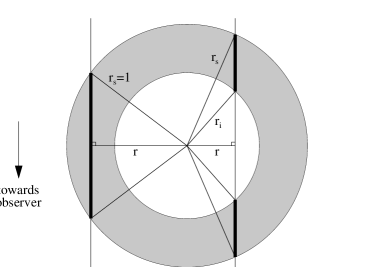
Figure 1: The geometry for a constant volume emissivity shell is shown. Two lines of sight through the shell are also shown. The surface brightness for these lines of sight is proportional to the length of the thick parts of the lines.

The geometry for the constant volume emissivity shell is shown in Fig. 1. Using this figure one can easily understand that the surface brightness for any given line of sight is proportional to the length of that part of the line that actually passes through the nebula. Hence for a constant emissivity shell the surface brightness profile is given by

$$\vspace{2.5mm}f(r)=\left\{\begin{array}[]{l@{\x{5}}l}2j_{\nu}\!\left(\sqrt{r_{\rm s}^{2}-r^{2}}-\sqrt{r_{\rm i}^{2}-r^{2}}\right)\hfil\hskip 14.22636pt&r\!\leq\!r_{\rm i}\!<\!r_{\rm s}\\ 2j_{\nu}\sqrt{r_{\rm s}^{2}-r^{2}}\hfil\hskip 14.22636pt&r_{\rm i}\!<\!r\!\leq\!r_{\rm s}\phantom{\hbox to0.0pt{$\left(\sqrt{r_{\rm s}^{2}}\right)$\hss}}\\ 0\hfil\hskip 14.22636pt&r_{\rm i}\!<\!r_{\rm s}\!<\!r\phantom{\hbox to0.0pt{$\left(\sqrt{r_{\rm s}^{2}}\right)$\hss}}\end{array}\right.\vspace{2.5mm}$$ (41)

Without loss of generality it can be assumed that $j_{\nu}=\frac{1}{4\pi}$ and $r_{\rm s}=1$. One can easily see that these profiles satisfy conditions (1) and (2c). First an analytic expression for $c_{2n}$ will be deduced by substituting Eq. (41) in Eq. (4)

$$c_{2n}=\left(\intop_{0}^{1}r^{2n+1}\sqrt{1-r^{2}}\mbox{\rm d}r-\intop_{0}^{r_{\rm i}}r^{2n+1}\sqrt{r_{\rm i}^{2}-r^{2}}\mbox{\rm d}r\right).$$

These integrals can be solved easily by using the substitution $t=r^{2}$ and give

$$c_{2n}=\sum_{k=0}^{n}\,(-1)^{k+n}\left(\!\!\begin{array}[]{c}n\\ k\end{array}\!\!\right)\frac{1-r_{\rm i}^{2n+3}}{2n+3-2k}.$$ (42)

The coefficients in the limiting case for an infinitely thin shell can also be calculated. After normalization to $c_{0}=1$ one finds

$$c_{2n}=\sum_{k=0}^{n}\,(-1)^{k+n}\left(\!\!\begin{array}[]{c}n\\ k\end{array}\!\!\right)\frac{2n+3}{2n+3-2k}.$$ (43)

Substituting Eq. (42) in Eq. (35) gives

$$\gamma(0)=\sqrt{\frac{5(1-r_{\rm i}^{3})}{2(1-r_{\rm i}^{5})\ln 2}}.$$ (44)

When Eq. (42) is substituted in Eq. (39) the following expression for the spherical case $r_{\rm i}$ = 0 is found (again giving additional terms without proof):

$$\gamma(\beta)=\sqrt{\frac{5}{2\ln 2}}\left(1-\frac{1}{7}\beta^{2}+\frac{5}{42}\beta^{4}-\frac{1157}{11319}\beta^{6}+\frac{2226013}{24720696}\beta^{8}-\frac{42074119}{519134616}\beta^{10}\right)+O(\beta^{12})\,(\beta\rightarrow 0).$$ (45)

When Eq. (43) is substituted in Eq. (39) one finds for the limiting case $r_{\rm i}\rightarrow 1$

$$\gamma(\beta)=\sqrt{\frac{3}{2\ln 2}}\left(1-\frac{1}{5}\beta^{2}+\frac{59}{350}\beta^{4}-\frac{128}{875}\beta^{6}+\frac{70117}{539000}\beta^{8}-\frac{20675393}{175175000}\beta^{10}\right)+O(\beta^{12})\,(\beta\rightarrow 0).$$ (46)

Inspection of both expressions suggests that the radius of convergence $B$ is approximately $B\approx 1$.

4 An alternative algorithm for determining the FWHM diameter

In this section, an expression will be derived that can be used to determine the fwhm diameter of an arbitrary surface brightness profile. This method will constitute an alternative algorithm to determine the fwhm diameter which is fully equivalent to a gaussian fit algorithm. The derivation will start with Eq. (34):

$$\sum_{n=0}^{\infty}(-1)^{n}\frac{c_{2n}\,\gamma^{2n}(\beta)\ln^{n}2}{n!}\sum_{k=0}^{n}\,(-1)^{k}\left(\!\!\begin{array}[]{c}n\\ k\end{array}\!\!\right)(\beta^{2}-2k)\,\beta^{2n-2}\left(\frac{\beta^{2}+1}{\beta^{2}+2}\right)^{k}=0.$$ (47)

This expression will be transformed into an expression for the conversion factor of the intrinsic surface brightness profile by taking the limit $\beta\rightarrow\infty$. This will be done by substituting $\beta=1/\epsilon$ and subsequently taking the limit $\epsilon\rightarrow 0$. First the innermost summation (which will be called $S_{n}$) will be evaluated.

$$S_{n}=\sum_{k=0}^{n}\,(-1)^{k}\left(\!\!\begin{array}[]{c}n\\ k\end{array}\!\!\right)\left(\frac{1}{\epsilon^{2}}-2k\right)\,\epsilon^{2-2n}\left(\frac{1+\epsilon^{2}}{1+2\epsilon^{2}}\right)^{k}=\sum_{k=0}^{n}\,(-1)^{k}\left(\!\!\begin{array}[]{c}n\\ k\end{array}\!\!\right)(1-2k\epsilon^{2})\,\epsilon^{-2n}\left[(1+\epsilon^{2})\sum_{l=0}^{\infty}(-1)^{l}\,2^{l}\,\epsilon^{2l}\right]^{k}=$$

$$\phantom{S_{n}}=\sum_{k=0}^{n}\,(-1)^{k}\left(\!\!\begin{array}[]{c}n\\ k\end{array}\!\!\right)(1-2k\epsilon^{2})\,\epsilon^{-2n}\left[1+\sum_{l=1}^{\infty}(-1)^{l}\,2^{l-1}\,\epsilon^{2l}\right]^{k}\equiv\sum_{k=0}^{n}\,(-1)^{k}\left(\!\!\begin{array}[]{c}n\\ k\end{array}\!\!\right)(1-2k\epsilon^{2})\,\epsilon^{-2n}\sum_{l=0}^{\infty}a_{k,l}\epsilon^{2l}.$$ (48)

The Taylor expansion of $(1+2\epsilon^{2})^{-1}$ has a radius of convergence of $\frac{1}{2}\sqrt{2}$, hence this derivation is only valid for $0\leq\epsilon<\frac{1}{2}\sqrt{2}$. The coefficients $a_{k,l}$ have been defined such that:

$$\left[1+\sum_{l=1}^{\infty}(-1)^{l}\,2^{l-1}\,\epsilon^{2l}\right]^{k}\equiv\sum_{l=0}^{\infty}a_{k,l}\epsilon^{2l}\hskip 8.53581pt\Rightarrow\hskip 8.53581pta_{k,0}=1;\hskip 8.53581pta_{k,l}=\frac{1}{l}\sum_{m=1}^{l}[\,m(k+1)-l\,]\,(-1)^{m}\,2^{m-1}\,a_{k,l-m}.$$ (49)

This expression for $a_{k,l}$ will yield a polynomial in $k$ of degree $l$, which will be written as (see Lemma A):

$$a_{k,l}=\sum_{i=0}^{l}d_{l,i}k^{i}=(-1)^{l}\frac{k^{l}}{l!}+\sum_{i=0}^{l-1}d_{l,i}k^{i}\equiv(-1)^{l}\frac{k^{l}}{l!}+b_{k,l}\hskip 8.53581pt{\rm for\ all\ }k,l\in{\mathbb{N}}_{0}{\rm\ and\ where\ }0^{0}\equiv 1.$$

Here $b_{k,l}$ represents the terms in $k$ with powers less than $l$ (if any). It can easily be shown that the series given by Eq. (49) is absolutely and uniformly convergent within its radius of convergence $\frac{1}{2}\sqrt{2}$. Hence it is allowed to substitute the last expression in Eq. (48) and reorder the summation:

$$S_{n}=\sum_{k=0}^{n}\,(-1)^{k}\left(\!\!\begin{array}[]{c}n\\ k\end{array}\!\!\right)(1-2k\epsilon^{2})\,\epsilon^{-2n}\sum_{l=0}^{\infty}\left[(-1)^{l}\frac{k^{l}}{l!}+b_{k,l}\right]\epsilon^{2l}=$$

$$\phantom{S_{n}}=\sum_{k=0}^{n}\,(-1)^{k}\left(\!\!\begin{array}[]{c}n\\ k\end{array}\!\!\right)\,\left[\sum_{l=0}^{\infty}(-1)^{l}\frac{k^{l}}{l!}\epsilon^{2l-2n}(1-2k\epsilon^{2})+\sum_{l=0}^{\infty}b_{k,l}\,\epsilon^{2l-2n}(1-2k\epsilon^{2})\right].$$

When the limit $\epsilon\rightarrow 0$ is taken, terms with $l>n$ will tend to zero, hence the following is true:

$$\lim_{\epsilon\rightarrow 0}S_{n}=\lim_{\epsilon\rightarrow 0}\sum_{k=0}^{n}\,(-1)^{k}\left(\!\!\begin{array}[]{c}n\\ k\end{array}\!\!\right)\,\left[\sum_{l=0}^{n}(-1)^{l}\frac{k^{l}}{l!}\epsilon^{2l-2n}(1-2k\epsilon^{2})+\sum_{l=0}^{n}b_{k,l}\,\epsilon^{2l-2n}(1-2k\epsilon^{2})\right].$$

When the order of the summation is reversed, this gives:

$$\lim_{\epsilon\rightarrow 0}S_{n}=\lim_{\epsilon\rightarrow 0}\sum_{l=0}^{n}\sum_{k=0}^{n}\,(-1)^{k}\left(\!\!\begin{array}[]{c}n\\ k\end{array}\!\!\right)\,(-1)^{l}\frac{k^{l}}{l!}\epsilon^{2l-2n}(1-2k\epsilon^{2})\ +\ \sum_{l=0}^{n}\sum_{k=0}^{n}\,(-1)^{k}\left(\!\!\begin{array}[]{c}n\\ k\end{array}\!\!\right)\,b_{k,l}\,\epsilon^{2l-2n}(1-2k\epsilon^{2})=$$

$$\phantom{\lim_{\epsilon\rightarrow 0}S_{n}}=\lim_{\epsilon\rightarrow 0}\sum_{l=0}^{n}(-1)^{l}\frac{\epsilon^{2l-2n}}{l!}\sum_{k=0}^{n}\,(-1)^{k}\left(\!\!\begin{array}[]{c}n\\ k\end{array}\!\!\right)k^{l}\ +\ \sum_{l=0}^{n-1}(-1)^{l+1}\frac{2\epsilon^{2l-2n+2}}{l!}\sum_{k=0}^{n}\,(-1)^{k}\left(\!\!\begin{array}[]{c}n\\ k\end{array}\!\!\right)k^{l+1}\ +$$

$$\phantom{\lim_{\epsilon\rightarrow 0}S_{n}=}+\ \sum_{l=0}^{n}\epsilon^{2l-2n}\sum_{k=0}^{n}(-1)^{k}\left(\!\!\begin{array}[]{c}n\\ k\end{array}\!\!\right)b_{k,l}\ -2\ \sum_{l=0}^{n-1}\epsilon^{2l-2n+2}\sum_{k=0}^{n}(-1)^{k}\left(\!\!\begin{array}[]{c}n\\ k\end{array}\!\!\right)k\,\,b_{k,l}.$$ (50)

When the well known result

$$\sum_{k=0}^{n}(-1)^{k}\left(\!\!\begin{array}[]{c}n\\ k\end{array}\!\!\right)k^{l}=(-1)^{n}\,n!\,\,\delta_{n,l}\hskip 8.53581pt{\rm for\ all\ }n,l\in{\mathbb{N}}_{0},\ l\leq n{\rm\ and\ where\ }0^{0}\equiv 1$$

is used, one can see that Eq. (50) can be written as

$$\lim_{\epsilon\rightarrow 0}S_{n}=\lim_{\epsilon\rightarrow 0}\sum_{l=0}^{n}(-1)^{l}\,\frac{\epsilon^{2l-2n}}{l!}\,(-1)^{n}\,n!\,\,\delta_{n,l}+\sum_{l=0}^{n-1}(-1)^{l+1}\,\frac{2\epsilon^{2l-2n+2}}{l!}\,(-1)^{n}\,n!\,\,\delta_{n,l+1}=1+\frac{2n!}{(n-1)!}=2n+1.$$ (51)

The last two summations in Eq. (50) evaluate to zero because $b_{k,l}$ only contains powers of $k$ up to $k^{l-1}$ or less. When Eq. (51) is substituted in Eq. (47) one finds the following result for the limit $\beta\rightarrow\infty$

$$\sum_{n=0}^{\infty}(-1)^{n}\,(2n+1)\,\frac{c_{2n}{\mathchoice{\kern 0.385pt\lower 2.39554pt\hbox{${}^{\prime}$}}{\kern 0.385pt\lower 2.39554pt\hbox{${}^{\prime}$}}{\lower 2.27109pt\hbox{${}^{\prime}$}}{\lower 2.27109pt\hbox{${}^{\prime}$}}}\,\gamma^{2n}\,\ln^{n}2}{n!}=0.$$ (52)

Which can be used to determine the limiting value of the conversion factor for any arbitrary surface brightness distribution. In the context of this section, an arbitrary surface brightness profile can mean an arbitrary observed profile, i.e. an intrinsic profile convolved with an arbitrary beam profile. To indicate this difference with previous definitions, primes have been added to the radial moments. When Eq. (2) is used, this expression can be rewritten into an expression which yields the fwhm of the observed profile directly:

$$\sum_{n=0}^{\infty}(-1)^{n}\,\frac{2n+1}{n!}\ c_{2n}{\mathchoice{\kern 0.385pt\lower 2.39554pt\hbox{${}^{\prime}$}}{\kern 0.385pt\lower 2.39554pt\hbox{${}^{\prime}$}}{\lower 2.27109pt\hbox{${}^{\prime}$}}{\lower 2.27109pt\hbox{${}^{\prime}$}}}\,\left(\frac{4\ln 2}{\Phi^{2}}\right)^{n}=0.$$ (53)

This implicit equation uses only the radial moments of the observed profile and can be solved easily using a Newton-Raphson scheme.

5 Determining diameters using second moments

It is well known that the fwhm of a gaussian is related to the second moment of a gaussian profile through:

$$\Phi_{2}=2\sqrt{\frac{c_{2}\,\ln 2}{c_{0}}}.$$ (54)

This formula is widely used to calculate the fwhm of an arbitrary profile. In general however, the result will not be identical to the fwhm derived from a gaussian fit. To distinguish the two values a subscript $2$ has been used. Since the definition of the fwhm is not identical, also the value for the conversion factor will be different. One can define (using Eq. 29)

$$\Phi_{\rm d}=\sqrt{\Phi_{2}^{2}-\Phi_{\rm b}^{2}(p)}\hskip 8.53581pt\Rightarrow\hskip 8.53581pt\gamma_{2}(\beta)=\frac{2}{\Phi_{\rm d}}=\left[\ln 2\left(\frac{c_{2}{\mathchoice{\kern 0.385pt\lower 2.39554pt\hbox{${}^{\prime}$}}{\kern 0.385pt\lower 2.39554pt\hbox{${}^{\prime}$}}{\lower 2.27109pt\hbox{${}^{\prime}$}}{\lower 2.27109pt\hbox{${}^{\prime}$}}}}{c_{0}{\mathchoice{\kern 0.385pt\lower 2.39554pt\hbox{${}^{\prime}$}}{\kern 0.385pt\lower 2.39554pt\hbox{${}^{\prime}$}}{\lower 2.27109pt\hbox{${}^{\prime}$}}{\lower 2.27109pt\hbox{${}^{\prime}$}}}}-\frac{1}{p}\right)\right]^{-\frac{1}{2}}.$$ (55)

To distinguish between the values of the radial moments for the unconvolved and the convolved profile, a prime has been used in the latter case. Now an expression for the radial moments of the convolved profile will be derived. Substituting Eq. (25) in Eq. (4) one finds

$$c_{2n}{\mathchoice{\kern 0.385pt\lower 2.39554pt\hbox{${}^{\prime}$}}{\kern 0.385pt\lower 2.39554pt\hbox{${}^{\prime}$}}{\lower 2.27109pt\hbox{${}^{\prime}$}}{\lower 2.27109pt\hbox{${}^{\prime}$}}}=2\pi\,a\sum_{k=0}^{\infty}c_{2k}\,p^{k}\sum_{l=0}^{k}\,(-1)^{k-l}\,\frac{p^{l}}{(k-l)!\,l!^{2}}\intop_{0}^{\infty}r^{2l+2n+1}\,\mbox{\rm e}^{-pr^{2}}\mbox{\rm d}r.$$ (56)

Here the order of summation and integration has been reversed; in Lemma A it is proven that this is allowed provided condition (2b) is fulfilled. The integral can evaluated easily using the substitution $s=r^{2}$ and yields

$$c_{2n}{\mathchoice{\kern 0.385pt\lower 2.39554pt\hbox{${}^{\prime}$}}{\kern 0.385pt\lower 2.39554pt\hbox{${}^{\prime}$}}{\lower 2.27109pt\hbox{${}^{\prime}$}}{\lower 2.27109pt\hbox{${}^{\prime}$}}}=\pi a\sum_{k=0}^{\infty}c_{2k}\,p^{k}\sum_{l=0}^{k}\,(-1)^{k-l}\,\frac{p^{l}}{(k-l)!\,l!^{2}}\frac{(l+n)!}{p^{l+n+1}}=\pi\frac{a}{p}\sum_{k=0}^{\infty}c_{2k}\,p^{k-n}\sum_{l=0}^{k}\,(-1)^{k-l}\,\frac{(l+n)!}{(k-l)!\,l!^{2}}.$$

The fact that the gaussian representing the beam should be normalized to 1 implies $a=p/\pi$. If $a_{n,i}$ is defined such that

$$\sum_{i=0}^{n}a_{n,i}\,l^{i}\equiv(l+n)\ldots(l+2)(l+1)=\frac{(l+n)!}{l!}\hskip 8.53581pt\hbox{for all }n,l\in{\mathbb{N}}_{0}\hbox{,\ and\ where\ }0^{0}\equiv 1\hskip 8.53581pt\Rightarrow$$

$$a_{n,0}=n!,\hskip 8.53581pta_{n,n}=1,\hskip 8.53581pta_{n,i}=na_{n-1,i}+a_{n-1,i-1}\hskip 8.53581pt\hbox{for all }n\in{\mathbb{N}}_{0},\hskip 2.84526pt1\leq i\leq n-1$$

one can write

$$c_{2n}{\mathchoice{\kern 0.385pt\lower 2.39554pt\hbox{${}^{\prime}$}}{\kern 0.385pt\lower 2.39554pt\hbox{${}^{\prime}$}}{\lower 2.27109pt\hbox{${}^{\prime}$}}{\lower 2.27109pt\hbox{${}^{\prime}$}}}=\sum_{k=0}^{\infty}c_{2k}\,\frac{p^{k-n}}{k!}\sum_{l=0}^{k}\,(-1)^{k-l}\,\frac{k!}{(k-l)!\,l!}\sum_{i=0}^{n}a_{n,i}\,l^{i}=\sum_{k=0}^{\infty}\frac{c_{2k}}{p^{n-k}}\,\sum_{i=0}^{n}(-1)^{k}\,\frac{a_{n,i}}{k!}\sum_{l=0}^{k}\,(-1)^{l}\,\left(\!\!\begin{array}[]{c}k\\ l\end{array}\!\!\right)\,l^{i}.$$

The innermost summation is well known and yields non-zero results only when $i\geq k$. Since $i\leq n$, this also implies $k\leq n$. Hence one can write

$$c_{2n}{\mathchoice{\kern 0.385pt\lower 2.39554pt\hbox{${}^{\prime}$}}{\kern 0.385pt\lower 2.39554pt\hbox{${}^{\prime}$}}{\lower 2.27109pt\hbox{${}^{\prime}$}}{\lower 2.27109pt\hbox{${}^{\prime}$}}}=\sum_{k=0}^{n}\frac{c_{2k}}{p^{n-k}}\,\sum_{i=k}^{n}(-1)^{k}\,\frac{a_{n,i}}{k!}\sum_{l=0}^{k}\,(-1)^{l}\,\left(\!\!\begin{array}[]{c}k\\ l\end{array}\!\!\right)\,l^{i}\equiv\sum_{k=0}^{n}b_{n,k}\frac{c_{2k}}{p^{n-k}}.$$

The following result will be postulated for the coefficients $b_{n,k}$

$$b_{n,k}=\sum_{i=k}^{n}(-1)^{k}\,\frac{a_{n,i}}{k!}\sum_{l=0}^{k}\,(-1)^{l}\,\left(\!\!\begin{array}[]{c}k\\ l\end{array}\!\!\right)\,l^{i}=\frac{n!^{2}}{(n-k)!\,k!^{2}}\hskip 8.53581pt\hbox{for all }n,k\in{\mathbb{N}}_{0},\hskip 2.84526ptk\leq n.$$

This expression has been checked numerically as was found to be correct for all $n,k\leq 19$. This makes it very plausible that it is correct for all $n$ and $k$. Substituting this result yields the following expression

$$c_{2n}{\mathchoice{\kern 0.385pt\lower 2.39554pt\hbox{${}^{\prime}$}}{\kern 0.385pt\lower 2.39554pt\hbox{${}^{\prime}$}}{\lower 2.27109pt\hbox{${}^{\prime}$}}{\lower 2.27109pt\hbox{${}^{\prime}$}}}=\sum_{k=0}^{n}\frac{n!^{2}}{(n-k)!\,k!^{2}}\,\frac{c_{2k}}{p^{n-k}}\hskip 8.53581pt\Rightarrow\hskip 8.53581ptc_{0}{\mathchoice{\kern 0.385pt\lower 2.39554pt\hbox{${}^{\prime}$}}{\kern 0.385pt\lower 2.39554pt\hbox{${}^{\prime}$}}{\lower 2.27109pt\hbox{${}^{\prime}$}}{\lower 2.27109pt\hbox{${}^{\prime}$}}}=c_{0},\hskip 8.53581ptc_{2}{\mathchoice{\kern 0.385pt\lower 2.39554pt\hbox{${}^{\prime}$}}{\kern 0.385pt\lower 2.39554pt\hbox{${}^{\prime}$}}{\lower 2.27109pt\hbox{${}^{\prime}$}}{\lower 2.27109pt\hbox{${}^{\prime}$}}}=\frac{c_{0}}{p}+c_{2},\hskip 8.53581ptc_{4}{\mathchoice{\kern 0.385pt\lower 2.39554pt\hbox{${}^{\prime}$}}{\kern 0.385pt\lower 2.39554pt\hbox{${}^{\prime}$}}{\lower 2.27109pt\hbox{${}^{\prime}$}}{\lower 2.27109pt\hbox{${}^{\prime}$}}}=\frac{2c_{0}}{p^{2}}+\frac{4c_{2}}{p}+c_{4},\hskip 8.53581pt\cdots$$ (57)

Substituting Eq. (57) in Eq. (55), one finds

$$\gamma_{2}(\beta)=\left[\ln 2\left(\frac{c_{2}{\mathchoice{\kern 0.385pt\lower 2.39554pt\hbox{${}^{\prime}$}}{\kern 0.385pt\lower 2.39554pt\hbox{${}^{\prime}$}}{\lower 2.27109pt\hbox{${}^{\prime}$}}{\lower 2.27109pt\hbox{${}^{\prime}$}}}}{c_{0}{\mathchoice{\kern 0.385pt\lower 2.39554pt\hbox{${}^{\prime}$}}{\kern 0.385pt\lower 2.39554pt\hbox{${}^{\prime}$}}{\lower 2.27109pt\hbox{${}^{\prime}$}}{\lower 2.27109pt\hbox{${}^{\prime}$}}}}-\frac{1}{p}\right)\right]^{-\frac{1}{2}}=\left[\ln 2\left(\frac{1}{p}+\frac{c_{2}}{c_{0}}-\frac{1}{p}\right)\right]^{-\frac{1}{2}}=\sqrt{\frac{c_{0}}{c_{2}\,\ln 2}}=\gamma(0).$$ (58)

Thus it has been proven that the conversion factor for second moment deconvolution is independent of beam size and equal to the conversion factor for gaussian deconvolution in the limit for infinitely large beams.

6 Conclusions and future work

In this work conversion factors have been determined to convert the deconvolved fwhm of a partially resolved nebula to its true diameter. This conversion factor depends on the fwhm of the beam and the intrinsic surface brightness distribution of the source. All work in this paper has been restricted to circularly symmetric surface brightness distributions and beams. The following results were obtained.

1. An implicit equation has been derived which can be used to determine the conversion factor given the intrinsic surface brightness distribution, the measured fwhm and the beam size.

2. From this implicit equation, various explicit expressions have been derived, which give the conversion factor in cases where the beam size is larger than the source.

3. Finally the implicit equation is used to construct an alternative algorithm for determining the fwhm of an arbitrary observed surface brightness distribution.

4. The fwhm derived with gaussian deconvolution is in general not equal to the fwhm derived with second moment deconvolution. Hence the conversion factors will also be different for both methods. The use of second moment deconvolution is studied for the first time in this paper and it is found that the conversion factor is independent of the beam size in this case. In the limit for infinitely large beam sizes, the values of the conversion factors for both methods are equal.

In a forthcoming publication the application of this theory to actual observations will be discussed (van Hoof 1999). Particular attention will be given to the limitations of the gaussian and second moment deconvolution method. Also a new method for deconvolving angular diameters will be presented.

Appendix A Additional proofs

In this section additional proofs for the existence and convergence of certain integrals and series will be presented.

Lemma 1

When $c_{n}$ exists, then also all $c_{i}$ exist with $i<n$.

PROOF. One can write

$$c_{i}=2\pi\!\intop_{0}^{\infty}f(r)\,r^{i+1}\mbox{\rm d}r=2\pi\!\intop_{0}^{1}f(r)\,r^{i+1}\mbox{\rm d}r+2\pi\!\intop_{1}^{\infty}f(r)\,r^{i+1}\mbox{\rm d}r\leq\frac{2\pi F}{i+2}+2\pi\!\intop_{1}^{\infty}f(r)\,r^{n+1}\mbox{\rm d}r\leq$$

$$\phantom{c_{i}}\leq\pi F+c_{n}-2\pi\!\intop_{0}^{1}f(r)\,r^{n+1}\mbox{\rm d}r\leq\pi F+c_{n}.$$

Since $f(r)r^{n+1}$ is positive everywhere. Hence the integral $c_{i}$ exists for all $i<n$.

Lemma 2

For $f(r)$ for which conditions (1) and (2c) are fulfilled, condition (2b) is also fulfilled.

PROOF. One can write

$$c_{2n}=2\pi\!\intop_{0}^{\infty}f(r)\,r^{2n+1}\mbox{\rm d}r=2\pi\!\intop_{0}^{R_{o}}f(r)\,r^{2n+1}\mbox{\rm d}r\leq 2\pi\,F\!\intop_{0}^{R_{o}}r^{2n+1}\mbox{\rm d}r=\frac{\pi\,F}{n+1}R_{o}^{2n+2}.$$

This proves that all $c_{2n}$ with $n\in{\mathbb{N}}_{0}$ exist. Now one can write

$$\lim_{n\rightarrow\infty}c_{2n}^{1/n}\leq\left(\frac{\pi\,F}{n+1}R_{o}^{2n+2}\right)^{1/n}=\lim_{n\rightarrow\infty}\left(\frac{\pi\,F\,R_{o}^{2}}{n+1}\right)^{1/n}\!\!R_{o}^{2}=R_{o}^{2}\hskip 8.53581pt\Rightarrow\hskip 8.53581pt\lim_{n\rightarrow\infty}c_{n}^{1/n}=R_{0}=o(n^{\frac{1}{2}})$$

and thus condition (2b) is fulfilled.

Lemma 3

The integral $I_{n,k,l}$ exists for all $n,k\in{\mathbb{N}}_{0}$ and all $l\in{\mathbb{N}}$ provided condition (1) is fulfilled. The integral $I_{n,k,0}$ exists for all $n\in{\mathbb{N}}_{0}$ and all $k\in{\mathbb{N}}$, provided that $c_{2n}$ exists and condition (1) is fulfilled.

PROOF. To prove the first part one can simply write

$$I_{n,k,l}=\intop_{0}^{\infty}f^{k}(r)g^{l}(r;a,p)\,r^{2n+1}\mbox{\rm d}r\leq a^{l}\,F^{k}\intop_{0}^{\infty}\mbox{\rm e}^{-lpr^{2}}r^{2n+1}\mbox{\rm d}r=\frac{a^{l}\,F^{k}\,n!}{2\,(lp)^{n+1}}.$$

To prove the second part one can write

$$I_{n,k,0}=\intop_{0}^{\infty}f^{k}(r)\,r^{2n+1}\mbox{\rm d}r\leq F^{k-1}\intop_{0}^{\infty}f(r)\,r^{2n+1}\mbox{\rm d}r=\frac{F^{k-1}}{2\pi}\,c_{2n},$$

and hence the integral exists if $c_{2n}$ exists.

Lemma 4

The integral $I_{n,k,l}$ is uniformly convergent for all $a,p\in(0,\infty)$, for any $n,k\in{\mathbb{N}}_{0}$ and any $l\in{\mathbb{N}}$, provided condition (1) is fulfilled.

PROOF. Lemma A proves that the integral $I_{n,k,l}$ exists. Now one can use

$$I^{\prime}_{n,k,l}=\intop_{X}^{Y}f^{k}(r)g^{l}(r;a,p)r^{2n+1}\mbox{\rm d}r\leq a^{l}F^{k}\intop_{X}^{Y}\mbox{\rm e}^{-lpr^{2}}r^{2n+1}\mbox{\rm d}r.$$

If the substitution $s=r^{2}$ is used, one finds

$$I^{\prime}_{n,k,l}\leq\frac{a^{l}F^{k}}{2}\intop_{X^{2}}^{Y^{2}}\mbox{\rm e}^{-lps}s^{n}\mbox{\rm d}s=\frac{a^{l}F^{k}}{2(lp)^{n+1}}\sum_{i=0}^{n}\frac{n!}{(n-i)!}\left[(lpX^{2})^{n-i}\,\mbox{\rm e}^{-lpX^{2}}-(lpY^{2})^{n-i}\,\mbox{\rm e}^{-lpY^{2}}\right].$$

Since $lpY^{2}>0$, one may write

$$I^{\prime}_{n,k,l}\leq\frac{a^{l}F^{k}}{2(lp)^{n+1}}\sum_{i=0}^{n}\frac{n!}{(n-i)!}(lpX^{2})^{n-i}\,\mbox{\rm e}^{-lpX^{2}}.$$

Since $n!/(n-i)!\leq n!$ and $(lpX^{2})^{n-i}\leq(lpX^{2})^{n}$ for $X\geq(lp)^{-\frac{1}{2}}$, one may write

$$I^{\prime}_{n,k,l}\leq\frac{a^{l}F^{k}}{2(lp)^{n+1}}\,(n+1)\,n!\,(lpX^{2})^{n}\,\mbox{\rm e}^{-lpX^{2}}=\frac{(n+1)!\,a^{l}F^{k}}{2lp}X^{2n}\,\mbox{\rm e}^{-lpX^{2}}.$$

It is well known that $\lim_{X\rightarrow\infty}X^{2n}\mbox{\rm e}^{-lpX^{2}}=0$ for any $n\in{\mathbb{N}}_{0}$, $l\in{\mathbb{N}}$ and $p\in(0,\infty)$. Hence one can always find a finite solution $X\geq(lp)^{-\frac{1}{2}}$ for the inequality

$$|I^{\prime}_{n,k,l}|<\epsilon\hskip 8.53581pt\Rightarrow\hskip 8.53581ptX^{2n}\mbox{\rm e}^{-lpX^{2}}<\frac{2lp\,\epsilon}{(n+1)!\,a^{l}\,F^{k}}$$

for all $\epsilon>0$, $n,k\in{\mathbb{N}}_{0}$, $l\in{\mathbb{N}}$ and $a,p\in(0,\infty)$. This proves that $I_{n,k,l}$ is uniformly convergent.

Lemma 5

In the expression given in Eq. (16) the order of summation and integration may be reversed for arbitrary values of $p$ and $r$, provided that conditions (1) and (2a) are fulfilled.

PROOF. Since the terms in Eq. (16) have alternating signs, the following partial sum will be considered

$$I_{N,R}=\sum_{n=0}^{N}\sum_{i=0}^{n}\intop_{0}^{R}\intop_{0}^{2\pi}\left|\,a\,\mbox{\rm e}^{-p(x^{2}+y^{2})}f(r{\mathchoice{\kern 0.385pt\lower 2.39554pt\hbox{${}^{\prime}$}}{\kern 0.385pt\lower 2.39554pt\hbox{${}^{\prime}$}}{\lower 2.27109pt\hbox{${}^{\prime}$}}{\lower 2.27109pt\hbox{${}^{\prime}$}}})\,\mbox{\rm e}^{-pr{\mathchoice{\kern 0.26949pt\lower 1.67688pt\hbox{${}^{\prime}$}}{\kern 0.26949pt\lower 1.67688pt\hbox{${}^{\prime}$}}{\lower 1.58975pt\hbox{${}^{\prime}$}}{\lower 1.58975pt\hbox{${}^{\prime}$}}}^{2}}\,(2p)^{n}\frac{x^{n-i}y^{i}}{(n-i)!\,i!}\,r{\mathchoice{\kern 0.385pt\lower 2.39554pt\hbox{${}^{\prime}$}}{\kern 0.385pt\lower 2.39554pt\hbox{${}^{\prime}$}}{\lower 2.27109pt\hbox{${}^{\prime}$}}{\lower 2.27109pt\hbox{${}^{\prime}$}}}^{n}\cos^{n-i}\!\varphi{\mathchoice{\kern 0.385pt\lower 2.39554pt\hbox{${}^{\prime}$}}{\kern 0.385pt\lower 2.39554pt\hbox{${}^{\prime}$}}{\lower 2.27109pt\hbox{${}^{\prime}$}}{\lower 2.27109pt\hbox{${}^{\prime}$}}}\,\sin^{i}\!\varphi{\mathchoice{\kern 0.385pt\lower 2.39554pt\hbox{${}^{\prime}$}}{\kern 0.385pt\lower 2.39554pt\hbox{${}^{\prime}$}}{\lower 2.27109pt\hbox{${}^{\prime}$}}{\lower 2.27109pt\hbox{${}^{\prime}$}}}\,r{\mathchoice{\kern 0.385pt\lower 2.39554pt\hbox{${}^{\prime}$}}{\kern 0.385pt\lower 2.39554pt\hbox{${}^{\prime}$}}{\lower 2.27109pt\hbox{${}^{\prime}$}}{\lower 2.27109pt\hbox{${}^{\prime}$}}}\right|\mbox{\rm d}\varphi{\mathchoice{\kern 0.385pt\lower 2.39554pt\hbox{${}^{\prime}$}}{\kern 0.385pt\lower 2.39554pt\hbox{${}^{\prime}$}}{\lower 2.27109pt\hbox{${}^{\prime}$}}{\lower 2.27109pt\hbox{${}^{\prime}$}}}\mbox{\rm d}r{\mathchoice{\kern 0.385pt\lower 2.39554pt\hbox{${}^{\prime}$}}{\kern 0.385pt\lower 2.39554pt\hbox{${}^{\prime}$}}{\lower 2.27109pt\hbox{${}^{\prime}$}}{\lower 2.27109pt\hbox{${}^{\prime}$}}}.$$

After changing $x$, $y$ to radial coordinates, one can write

$$I_{N,R}\leq\sum_{n=0}^{N}\sum_{i=0}^{n}\intop_{0}^{R}\intop_{0}^{2\pi}a\,(2p)^{n}\frac{r^{n}}{(n-i)!\,i!}\,f(r{\mathchoice{\kern 0.385pt\lower 2.39554pt\hbox{${}^{\prime}$}}{\kern 0.385pt\lower 2.39554pt\hbox{${}^{\prime}$}}{\lower 2.27109pt\hbox{${}^{\prime}$}}{\lower 2.27109pt\hbox{${}^{\prime}$}}})\,r{\mathchoice{\kern 0.385pt\lower 2.39554pt\hbox{${}^{\prime}$}}{\kern 0.385pt\lower 2.39554pt\hbox{${}^{\prime}$}}{\lower 2.27109pt\hbox{${}^{\prime}$}}{\lower 2.27109pt\hbox{${}^{\prime}$}}}^{n+1}\mbox{\rm d}\varphi{\mathchoice{\kern 0.385pt\lower 2.39554pt\hbox{${}^{\prime}$}}{\kern 0.385pt\lower 2.39554pt\hbox{${}^{\prime}$}}{\lower 2.27109pt\hbox{${}^{\prime}$}}{\lower 2.27109pt\hbox{${}^{\prime}$}}}\mbox{\rm d}r{\mathchoice{\kern 0.385pt\lower 2.39554pt\hbox{${}^{\prime}$}}{\kern 0.385pt\lower 2.39554pt\hbox{${}^{\prime}$}}{\lower 2.27109pt\hbox{${}^{\prime}$}}{\lower 2.27109pt\hbox{${}^{\prime}$}}}=\sum_{n=0}^{N}\sum_{i=0}^{n}\intop_{0}^{R}2\pi a\,(2p)^{n}\frac{r^{n}}{n!}\left(\!\!\begin{array}[]{c}n\\ i\end{array}\!\!\right)f(r{\mathchoice{\kern 0.385pt\lower 2.39554pt\hbox{${}^{\prime}$}}{\kern 0.385pt\lower 2.39554pt\hbox{${}^{\prime}$}}{\lower 2.27109pt\hbox{${}^{\prime}$}}{\lower 2.27109pt\hbox{${}^{\prime}$}}})\,r{\mathchoice{\kern 0.385pt\lower 2.39554pt\hbox{${}^{\prime}$}}{\kern 0.385pt\lower 2.39554pt\hbox{${}^{\prime}$}}{\lower 2.27109pt\hbox{${}^{\prime}$}}{\lower 2.27109pt\hbox{${}^{\prime}$}}}^{n+1}\mbox{\rm d}r{\mathchoice{\kern 0.385pt\lower 2.39554pt\hbox{${}^{\prime}$}}{\kern 0.385pt\lower 2.39554pt\hbox{${}^{\prime}$}}{\lower 2.27109pt\hbox{${}^{\prime}$}}{\lower 2.27109pt\hbox{${}^{\prime}$}}}=$$

$$\phantom{I_{N,R}}=\sum_{n=0}^{N}\sum_{i=0}^{n}2\pi a\,\frac{(2pr)^{n}}{n!}\left(\!\!\begin{array}[]{c}n\\ i\end{array}\!\!\right)\intop_{0}^{R}f(r{\mathchoice{\kern 0.385pt\lower 2.39554pt\hbox{${}^{\prime}$}}{\kern 0.385pt\lower 2.39554pt\hbox{${}^{\prime}$}}{\lower 2.27109pt\hbox{${}^{\prime}$}}{\lower 2.27109pt\hbox{${}^{\prime}$}}})\,r{\mathchoice{\kern 0.385pt\lower 2.39554pt\hbox{${}^{\prime}$}}{\kern 0.385pt\lower 2.39554pt\hbox{${}^{\prime}$}}{\lower 2.27109pt\hbox{${}^{\prime}$}}{\lower 2.27109pt\hbox{${}^{\prime}$}}}^{n+1}\mbox{\rm d}r{\mathchoice{\kern 0.385pt\lower 2.39554pt\hbox{${}^{\prime}$}}{\kern 0.385pt\lower 2.39554pt\hbox{${}^{\prime}$}}{\lower 2.27109pt\hbox{${}^{\prime}$}}{\lower 2.27109pt\hbox{${}^{\prime}$}}}\leq\sum_{n=0}^{N}\sum_{i=0}^{n}2\pi a\,\frac{(2pr)^{n}}{n!}\left(\!\!\begin{array}[]{c}n\\ i\end{array}\!\!\right)c_{n},$$

where for the last step condition (1) has been used. Since it is assumed that $c_{2n}$ exists for all $n\in{\mathbb{N}}_{0}$, this implies that $c_{n}$ exists for all $n\in{\mathbb{N}}_{0}$ (Lemma A). Hence $I_{N,R}$ exists for arbitrary $N$ and $R$. This also proves that $\lim_{R\rightarrow\infty}I_{N,R}$ exists. For arbitrary $R$ the following is true

$$I_{N,R}\leq\sum_{n=0}^{N}2\pi a\,\frac{(2pr)^{n}}{n!}\,c_{n}\sum_{i=0}^{n}\left(\!\!\begin{array}[]{c}n\\ i\end{array}\!\!\right)=\sum_{n=0}^{N}2\pi a\,\frac{(2pr)^{n}}{n!}\,c_{n}\,2^{n}=\sum_{n=0}^{N}2\pi a\,\frac{(4pr)^{n}}{n!}\,c_{n}\equiv\sum_{n=0}^{N}a_{n}.$$

In order for $\lim_{N\rightarrow\infty}I_{N,R}$ to exist, the following must be true

$$\lim_{n\rightarrow\infty}a_{n}^{1/n}=\lim_{n\rightarrow\infty}\left[2\pi a\frac{(4pr)^{n}}{n!}\,c_{n}\right]^{1/n}<\lim_{n\rightarrow\infty}\left[2\pi a\frac{(4p\,\mbox{\rm e}\,r)^{n}}{n^{n}}c_{n}\right]^{1/n}=\lim_{n\rightarrow\infty}(2\pi a)^{1/n}\frac{4p\,\mbox{\rm e}\,r}{n}c_{n}^{1/n}=\lim_{n\rightarrow\infty}\frac{4p\,\mbox{\rm e}\,r}{n}c_{n}^{1/n}<1.$$

Here the well known result $n!>\mbox{\rm e}^{-n}n^{n}$ for all $n>0$ has been used. In order for the last inequality to be true for arbitrary values of $p$ and $r$, the constraint $c_{n}^{1/n}=o(n)\,(n\rightarrow\infty)$ has to be imposed. This proves that $\lim_{N\rightarrow\infty}I_{N,R}$ exists. Since the argument given above is also valid in the limit $R\rightarrow\infty$, this also proves that $\lim_{N,R\rightarrow\infty}I_{N,R}$ exists. This completes the proof that the order of integration and summation in Eq. (16) may be reversed.

Lemma 6

The series given in Eq. (21) is absolutely and uniformly convergent for all $r\in[0,\infty)$ and $p\in[0,\infty)$, provided that conditions (1) and (2a) are fulfilled.

PROOF. First it will be proven that these conditions imply $[c_{n}(p)]^{1/n}=o(n)\,(n\rightarrow\infty)$ for all $p\in[\,0,\infty\,)$. Since $f(r)\geq 0$ everywhere, one can write

$$c_{2n}(p)=2\pi\!\intop_{0}^{\infty}f(r)\,r^{2n+1}\mbox{\rm e}^{-pr^{2}}\mbox{\rm d}r\leq 2\pi\!\intop_{0}^{\infty}f(r)\,r^{2n+1}\mbox{\rm d}r=c_{2n}.$$

This proves that $c_{2n}(p)$ exists for all $n\in{\mathbb{N}}_{0}$ and all $p\in[\,0,\infty\,)$. It also implies

$$[c_{n}(p)]^{1/n}\leq c_{n}^{1/n}=o(n)\,(n\rightarrow\infty),$$

for all $p\in[\,0,\infty\,)$, which completes the first step. The summation in Eq. (21) is a Taylor series, which will have an infinite radius of convergence when the following condition is fulfilled

$$\lim_{n\rightarrow\infty}\left[\frac{c_{2n}(p)p^{2n}}{n!^{2}}\right]^{1/(2n)}<\lim_{n\rightarrow\infty}\left[\frac{c_{2n}(p)(p\,\mbox{\rm e})^{2n}}{n^{2n}}\right]^{1/(2n)}=\lim_{n\rightarrow\infty}\frac{p\,\mbox{\rm e}}{n}\,[c_{2n}(p)]^{1/(2n)}=0.$$

Here the well known result $n!>\mbox{\rm e}^{-n}n^{n}$ for all $n>0$ has been used. For the last condition to hold for any arbitrary value of $p$, it must be true that $[c_{2n}(p)]^{1/(2n)}=o(n)\,(n\rightarrow\infty)$ or $[c_{n}(p)]^{1/n}=o(n)\,(n\rightarrow\infty)$, which has been proven to be true. Any Taylor series is absolutely and uniformly convergent within its radius of convergence. Since the gaussian in Eq. (21) is bounded for all $p,r\in[0,\infty)$, this also proves that the expression in Eq. (21) is absolutely and uniformly convergent for all $p,r\in[0,\infty)$.

Lemma 7

In the expression given in Eq. (22) the order of summation and integration may be reversed for arbitrary values of $p$, provided that conditions (1) and (2b) are fulfilled.

PROOF. Since the terms in Eq. (22) have alternating signs, the following partial sum will be considered

$$I_{K,R}=\sum_{k=0}^{K}\intop_{0}^{R}\left|\,2\pi\,(-1)^{k}\,\frac{p^{k}}{k!}\,f(r)\,r^{n+2k+1}\right|\mbox{\rm d}r=\sum_{k=0}^{K}2\pi\,\frac{p^{k}}{k!}\intop_{0}^{R}f(r)\,r^{n+2k+1}\mbox{\rm d}r\leq\sum_{k=0}^{K}2\pi\,\frac{p^{k}}{k!}\,c_{n+2k}\equiv\sum_{k=0}^{K}a_{k},$$

where for the last inequality condition (1) has been used. Since it is assumed that $c_{2n}$ exists for all $n\in{\mathbb{N}}_{0}$, this implies that $c_{n}$ exists for all $n\in{\mathbb{N}}_{0}$ (Lemma A). From this it is clear that $I_{K,R}$ exists for arbitrary values of $K$ and $R$. It is also clear that $\lim_{R\rightarrow\infty}I_{K,R}$ exists for any value of $K$. In order for $\lim_{K\rightarrow\infty}I_{K,R}$ to exist, the following must be true

$$\lim_{k\rightarrow\infty}a_{k}^{1/k}=\lim_{k\rightarrow\infty}\left(2\pi\,\frac{p^{k}}{k!}\,c_{n+2k}\right)^{1/k}<\lim_{k\rightarrow\infty}\left[2\pi\,\frac{(p\,\mbox{\rm e})^{k}}{k^{k}}\,c_{n+2k}\right]^{1/k}=\lim_{k\rightarrow\infty}(2\pi)^{1/k}\,\frac{p\,\mbox{\rm e}}{k}\,c_{n+2k}^{1/k}=\lim_{k\rightarrow\infty}\frac{p\,\mbox{\rm e}}{k}\,c_{2k}^{1/k}<1.$$

Here the well known result $k!>\mbox{\rm e}^{-k}k^{k}$ for all $k>0$ has been used. In order for the last inequality to be true for arbitrary values of $p$, the constraint $c_{2k}^{1/k}=o(k)\,(k\rightarrow\infty)$ has to be imposed. Using the substitution $n=2k$, this can be written as $c_{n}^{1/n}=o(n^{\frac{1}{2}})\,(n\rightarrow\infty)$. This completes the proof that $\lim_{K\rightarrow\infty}I_{K,R}$ exists. Since the argument given above is also valid in the limit $R\rightarrow\infty$ this also proves that $\lim_{K,R\rightarrow\infty}I_{K,R}$ exists. This completes the proof that the order of integration and summation in Eq. (22) may be reversed.

Lemma 8

The series given in Eq. (23) is absolutely and uniformly convergent for all $p\in[0,\infty)$, provided condition (2b) is fulfilled.

PROOF. The summation in Eq. (23) is a Taylor series in $p$, which will have an infinite radius of convergence when the following criterion is fulfilled

$$\lim_{k\rightarrow\infty}\left(\frac{c_{n+2k}}{k!}\right)^{1/k}<\lim_{k\rightarrow\infty}\left(\frac{\mbox{\rm e}^{k}}{k^{k}}\,c_{n+2k}\right)^{1/k}=\lim_{k\rightarrow\infty}\frac{\mbox{\rm e}}{k}\,c_{n+2k}^{1/k}=\lim_{k\rightarrow\infty}\frac{\mbox{\rm e}}{k}\,c_{2k}^{1/k}=0.$$

Here the well known result $k!>\mbox{\rm e}^{-k}k^{k}$ for all $k>0$ has been used. Condition (2b) assures that this is true, which can be seen by making the transformation $n=2k$. This proves that the series has an infinite radius of convergence. Since any Taylor series is absolutely and uniformly convergent within its radius of convergence, this completes the proof.

Lemma 9

In the expression given in Eq. (27) the order of summation and integration may be reversed for arbitrary values of $p$, provided that condition (2b) is fulfilled.

PROOF. Since the terms in Eq. (27) don’t always have the same sign, the following partial sum will be considered

$$I_{N,S}=\sum_{n=0}^{N}\,\intop_{0}^{S}\left|\,(1-2s)\,\mbox{\rm e}^{-\zeta s}c_{2n}p^{n}\sum_{k=0}^{n}(-1)^{n-k}\frac{(\zeta-1)^{k}}{(n-k)!\,k!^{2}}s^{k}\right|\mbox{\rm d}s\leq\sum_{n=0}^{N}c_{2n}\,p^{n}\sum_{k=0}^{n}\,\frac{(\zeta-1)^{k}}{(n-k)!\,k!^{2}}\intop_{0}^{S}(2s+1)\,s^{k}\,\mbox{\rm e}^{-\zeta s}\mbox{\rm d}s\leq$$

$$\phantom{I_{N,S}}\leq\sum_{n=0}^{N}\,c_{2n}\,p^{n}\sum_{k=0}^{n}\,\frac{(\zeta-1)^{k}}{(n-k)!\,k!^{2}}\left[2\frac{(k+1)!}{\zeta^{k+2}}+\frac{k!}{\zeta^{k+1}}\right]\leq\sum_{n=0}^{N}\,\frac{c_{2n}\,p^{n}}{\zeta^{2}}\sum_{k=0}^{n}\,\frac{\zeta+2k+2}{(n-k)!\,k!}\leq$$

$$\phantom{I_{N,S}}\leq\sum_{n=0}^{N}\,\frac{c_{2n}\,p^{n}}{n!}\frac{(\zeta+2n+2)}{\zeta^{2}}\sum_{k=0}^{n}\,\left(\!\!\begin{array}[]{c}n\\ k\end{array}\!\!\right)=\sum_{n=0}^{N}\,\frac{c_{2n}\,(2p)^{n}}{n!}\frac{(\zeta+2n+2)}{\zeta^{2}}\equiv\sum_{n=0}^{N}a_{n}.$$

Here the fact has been used that $\zeta>1$ (see Eq. 32) and hence $(\zeta-1)^{k}<\zeta^{k}$. Since it is assumed that $c_{2n}$ exists for all $n\in{\mathbb{N}}_{0}$, it is clear that $I_{N,S}$ exists for arbitrary values of $N$ and $S$. It is also clear that $\lim_{S\rightarrow\infty}I_{N,S}$ exists. In order for $\lim_{N\rightarrow\infty}I_{N,S}$ to exist, the following must be true

$$\lim_{n\rightarrow\infty}a_{n}^{1/n}=\lim_{n\rightarrow\infty}\left[\frac{c_{2n}\,(2p)^{n}}{n!}\frac{(\zeta+2n+2)}{\zeta^{2}}\right]^{1/n}<\lim_{n\rightarrow\infty}\left[\frac{c_{2n}\,(2p\,\mbox{\rm e})^{n}}{n^{n}}\frac{(\zeta+2n+2)}{\zeta^{2}}\right]^{1/n}=$$

$$\phantom{\lim_{n\rightarrow\infty}a_{n}^{1/n}}=\lim_{n\rightarrow\infty}\left[c_{2n}\frac{(\zeta+2n+2)}{\zeta^{2}}\right]^{1/n}\frac{2p\,\mbox{\rm e}}{n}=\lim_{n\rightarrow\infty}c_{2n}^{1/n}\frac{2p\,\mbox{\rm e}}{n}<1.$$

Here the well known result $n!>\mbox{\rm e}^{-n}n^{n}$ for all $n>0$ has been used. In order for the last inequality to be true for arbitrary values of $p$, the constraint $c_{2n}^{1/n}=o(n)\,(n\rightarrow\infty)$ has to be imposed. Using the substitution $2n\rightarrow n$, this can be written as $c_{n}^{1/n}=o(n^{\frac{1}{2}})\,(n\rightarrow\infty)$. This completes the proof that $\lim_{N\rightarrow\infty}I_{N,S}$ exists. Since the argument given above is also valid in the limit $S\rightarrow\infty$ this also proves that $\lim_{N,S\rightarrow\infty}I_{N,S}$ exists. This completes the proof that the order of integration and summation in Eq. (27) may be reversed.

Lemma 10

The expression for $a_{k,l}$ given in Eq. (49) yields a polynomial in $k$ of degree $l$ for all $l\in{\mathbb{N}}_{0}$.

PROOF. From the definition given in Eq. (49) it is clear that the lemma is correct for $l=0$. If it is assumed that the lemma is correct for all $l^{\prime}<l$ then the last part of Eq. (49) assures that $a_{k,l}$ is equal to the sum of $l$ polynomials of degree $l^{\prime}=l-1,\ l-2,\ \ldots$, multiplied by a linear term in $k$. This yields a polynomial of degree $\max(l^{\prime}+1)=l$. Since the lemma is true for $l=0$, this proves by induction that the lemma is true for all $l\in{\mathbb{N}}_{0}$.

Now an expression for the highest order term of this polynomial will be derived. It is clear that the highest order contribution to $a_{k,l}$ only comes from the term with $m=1$ in Eq. (49). If one defines

$$a_{k,l}=\sum_{i=0}^{l}d_{l,i}k^{i},$$

one can deduce the following expression for $d_{l,l}$ from Eq. (49)

$$d_{l,l}=-\frac{k}{l}d_{l-1,l-1}=\frac{k^{2}}{l(l-1)}d_{l-2,l-2}=\left[\prod_{i=0}^{l}(-1)\frac{k}{i}\right]d_{0,0}=(-1)^{l}\frac{k^{l}}{l!}\hskip 8.53581pt\Rightarrow\hskip 8.53581pta_{k,l}=(-1)^{l}\frac{k^{l}}{l!}+\sum_{i=0}^{l-1}d_{l,i}k^{i}\equiv(-1)^{l}\frac{k^{l}}{l!}+b_{k,l}.$$

Here $b_{k,l}$ is the lower order remainder of $a_{k,l}$ which is a polynomial of degree $l-1$ or less in $k$. It can easily be checked that these expressions are also valid for $k=0$ and $l=0$ if one postulates $0^{0}\equiv 1$ and $b_{k,0}\equiv 0$.

Lemma 11

In the expression given in Eq. (56) the order of summation and integration may be reversed for arbitrary values of $p$, provided that condition (2b) is fulfilled.

PROOF. Since the terms in Eq. (56) have alternating signs, the following partial sum will be considered

$$I_{K,R}=\sum_{k=0}^{K}\intop_{0}^{R}\left|\,2\pi\,ac_{2k}p^{k}\sum_{l=0}^{k}\,(-1)^{k-l}\,\frac{p^{l}}{(k-l)!\,l!^{2}}r^{2l+2n+1}\,\mbox{\rm e}^{-pr^{2}}\right|\mbox{\rm d}r=\sum_{k=0}^{K}\,2\pi a\,c_{2k}\,p^{k}\sum_{l=0}^{k}\,\frac{p^{l}}{(k-l)!\,l!^{2}}\intop_{0}^{R}r^{2l+2n+1}\,\mbox{\rm e}^{-pr^{2}}\mbox{\rm d}r\leq$$

$$\phantom{I_{K,R}}\leq\sum_{k=0}^{K}\,\pi a\,c_{2k}\,p^{k}\sum_{l=0}^{k}\,\frac{p^{l}}{(k-l)!\,l!^{2}}\frac{(l+n)!}{p^{l+n+1}}=\sum_{k=0}^{K}\,\pi\frac{a}{p}\,c_{2k}\,p^{k-n}\sum_{l=0}^{k}\,\frac{(l+n)!}{(k-l)!\,l!^{2}}=\sum_{k=0}^{K}\,c_{2k}\,p^{k-n}\sum_{l=0}^{k}\,\frac{k!}{(k-l)!\,l!}\frac{(l+n)!}{l!\,k!}\leq$$

$$\phantom{I_{K,R}}\leq\sum_{k=0}^{K}\,c_{2k}\,p^{k-n}\sum_{l=0}^{k}\left(\!\!\begin{array}[]{c}k\\ l\end{array}\!\!\right)\frac{(l+n)^{n}}{k!}\leq\sum_{k=0}^{K}\,c_{2k}\,p^{k-n}\frac{(k+n)^{n}}{k!}\sum_{l=0}^{k}\left(\!\!\begin{array}[]{c}k\\ l\end{array}\!\!\right)=\sum_{k=0}^{K}\,c_{2k}\,p^{k-n}\frac{2^{k}\,(k+n)^{n}}{k!}\equiv\sum_{k=0}^{K}a_{k}.$$

In this derivation it has been used that the gaussian used to convolve the profile should be normalized to 1, this implies $a=p/\pi$. Since it is assumed that $c_{2k}$ exists for all $k\in{\mathbb{N}}_{0}$, this proves that $I_{K,R}$ exists for arbitrary values of $K$ and $R$. It also proves that $\lim_{R\rightarrow\infty}I_{K,R}$ exists for arbitrary values of $K$. In order for $\lim_{K\rightarrow\infty}I_{K,R}$ to exist, the following must be true

$$\lim_{k\rightarrow\infty}a_{k}^{1/k}=\lim_{k\rightarrow\infty}\left[c_{2k}\,p^{k-n}\frac{2^{k}\,(k+n)^{n}}{k!}\right]^{1/k}=\lim_{k\rightarrow\infty}\left[c_{2k}\left(\frac{k+n}{p}\right)^{n}\frac{(2p)^{k}}{k!}\right]^{1/k}<\lim_{k\rightarrow\infty}\left[c_{2k}\left(\frac{k+n}{p}\right)^{n}\frac{(2p\,\mbox{\rm e})^{k}}{k^{k}}\right]^{1/k}=$$

$$\phantom{\lim_{k\rightarrow\infty}a_{k}^{1/k}}=\lim_{k\rightarrow\infty}c_{2k}^{1/k}\left(\frac{k+n}{p}\right)^{n/k}\frac{2p\,\mbox{\rm e}}{k}=\lim_{k\rightarrow\infty}c_{2k}^{1/k}\,\frac{2p\,\mbox{\rm e}}{k}<1.$$

Here the well known result $k!>\mbox{\rm e}^{-k}k^{k}$ for all $k>0$ has been used. In order for the last inequality to be true for arbitrary values of $p$, the constraint $c_{2k}^{1/k}=o(k)\,(k\rightarrow\infty)$ has to be imposed. Using the substitution $n=2k$, this can be written as $c_{n}^{1/n}=o(n^{\frac{1}{2}})\,(n\rightarrow\infty)$. This completes the proof that $\lim_{K\rightarrow\infty}I_{K,R}$ exists. Since the argument given above is also valid in the limit $R\rightarrow\infty$ this also proves that $\lim_{K,R\rightarrow\infty}I_{K,R}$ exists. This completes the proof that the order of integration and summation in Eq. (56) may be reversed.

Appendix B Symbols

The following definitions for the symbols have been used.

$a$ – Measure for the height of the gaussian.

$c_{n}$ – Radial moments of the surface brightness profile. Defined in Eq. (4).

$c_{n}(p)$ – Generalized radial moments of the surface brightness profile. Defined in Eq. (20).

$f(r)$ – The surface brightness profile of the nebula.

$F$ – Upper bound for the surface brightness profile.

$g(r;a,p)$ – Two-dimensional gaussian profile.

$j_{\nu}$ – The emissivity per unit frequency.

$L_{n}$ – Laguerre polynomial of degree $n$.

$p$ – Measure for the width of a gaussian. Related to the fwhm through Eq. (29).

$r$ – Polar coordinate on the sky. Subscripts have the following meaning:
$i$ – the inner radius of the nebula,
$s$ – the Strömgren or outer radius of the nebula.

$x$,$y$ – Cartesian coordinates on the sky.

$\beta$ – Ratio of the deconvolved fwhm diameter of the nebula to the fwhm of the beam.

$\gamma$ – Factor to convert the deconvolved fwhm to the true angular diameter. Subscripts have the following meaning:
$<$none$>$ – gaussian fits were used to determine the fwhm
$2$ – second moments were used to determine the fwhm (Eq. 55).
$f$ – indicates the fitting function used to approximate $\gamma(\beta)$.

$\Gamma$ – The gamma function.

$\delta_{i,j}$ – Kronecker delta symbol.

$\zeta$ – Auxiliary variable, related to $\beta$ through Eq. (32).

$\Theta_{\rm d}$ – True angular diameter of the nebula ($\Theta_{\rm d}\equiv 2r_{\rm s}$).

$\varphi$ – Polar coordinate on the sky.

$\Phi$ – The fwhm diameter of a profile. Subscripts have the following meaning:
$<$none$>$ – indicates the fwhm of a gaussian profile,
$b$ – indicates the fwhm of the beam,
$d$ – indicates the deconvolved fwhm of a profile (defined in Eq. 30 or Eq. 55),
$2$ – indicates the fwhm of a profile obtained using second moments (Eq. 54).

Other symbols have varying meanings as defined in the pertinent sections.

References

- [1]
- [1994] Bedding T.R., Zijlstra A.A., 1994, A&A, 283, 955 (BZ)
- [1967] Mezger P.G., Henderson A.P., 1967, ApJ 147, 471 (MH)
- [1978] Panagia N., Walmsley C.M., 1978, A&A 70, 411 (PW)
- [1996] Schneider S.E., Buckley D., 1996, ApJ 459, 606 (SB)
- [1999] van Hoof P.A.M., 1999, MNRAS, submitted
- [1997] Wellman G.F., Daly R.A., Wan L., 1997, ApJ 480, 79