A Preferred-Direction Statistic for Sky Maps

Abstract

Large patterns could exist on the microwave sky as a result of various non-standard possibilities for the large-scale Universe – rotation or shear, non-trivial topology, and single topological defects are specific examples. All-sky (or nearly all-sky) CMB data sets allow us, uniquely, to constrain such exotica, and it is therefore worthwhile to explore a wide range of statistical tests. We describe one such statistic here, which is based on determining gradients and is useful for assessing the level of ‘preferred directionality’ or ‘stripiness’ in the map. This method is more general than other techniques for picking out specific patterns on the sky, and it also has the advantage of being easily calculable for the mega-pixel maps which will soon be available. For the purposes of illustration, we apply this statistic to the four-year COBE DMR data. For future CMB maps we expect this to be a useful statistical test of the large scale structure of the Universe. In principle, the same statistic could also be applied to sky maps at other wavelengths, to CMB polarisation maps, and to catalogues of discrete objects. It may also be useful as a means of checking for residual directionality (e.g., from Galactic or ecliptic signals) in maps.

1 Introduction

The desire to understand the nature of the physical universe has driven scientific inquiry throughout history. An important aspect of this has been the search for models which accurately describe the structure of the Universe on the very largest scales. Only in the last decade have we had the means to access information from the largest of the scales that are observationally within reach, namely those scales corresponding to the light-crossing time in the age of the Universe.

In the absence of a unique mathematical description for the structure of space, the only way to pin down its large-scale behaviour is through direct observation of features which probe the largest scales. Anisotropies in the Cosmic Microwave Background (CMB) give us just such a diagnostic tool. Furthermore, since the detection of large-angle anisotropies by the COBE DMR experiment [Smoot et al. 1992] it is now clear that this is a tool that can be used in practice. Although the COBE detection was impressive, the limited angular resolution and sensitivity make the data set far from definitive. Future CMB experiments, and in particular the Microwave Anisotropy Probe (MAP) and Planck satellites will provide data that will be far more constraining for the structure of the Universe.

The traditional view is that most of the information content in the CMB sky is contained in the angular power spectrum of anisotropies. As a result, a great deal of effort has gone into obtaining the best estimate of the power spectrum from the COBE DMR data [Bennett et al. 1996, Górski et al. 1996, White & Bunn 1995, Bond 1996], as well as for other experiments. However, it is certainly possible that the CMB sky exhibits some large-scale pattern, not discernible from the power spectrum, which would indicate some non-trivial large-scale structure. Since the endeavour of examining the Universe on its largest accessible scales is such a grand one, it is certainly worthwhile to explore all statistics which might be used to constrain such patterns.

Examples of specific such patterns have already been investigated, although we would like to stress that the current list is likely to be far from exhaustive, and the best approach is the empirical one: simply look to see if there are surprises in the data. Already much effort has gone into examining the consequences of non-trivial topology, with a repetition scale close to the Hubble radius today [Stevens et al. 1993, de Oliveira-Costa et al. 1996, Levin et al. 1997, Cornish et al. 1998, Souradeep et al. 1998]. One manifestation of a short periodicity scale in two direction is that the sky would appear to be composed of concentric ‘stripes,’ superimposed on the background of fluctuations [Starobinsky 1993]. Another class of possibilities are universes with rotation or shear, which define a preferred direction on the sky around which there can be special patterns [Barrow, Juszkiewicz, & Sonoda 1985]; specific Bianchi models have been investigated in detail [Bunn et al. 1996, Kogut et al. 1997]. A further example is the possibility that single large-scale topological defects could give rise to particular patterns, e.g., a step-like discontinuity caused by the largest cosmic string [Perivolaropoulos 1998], or a localised pattern caused by the last texture to unwind [Magueijo 1995]. It is also possible that properties of particle fields in the Universe could create electromagnetic effects yielding special directions (see e.g. Carroll & Field 1997 for a recent discussion). These examples represent the cases already studied, where there are known patterns which exhibit some directionality. We wish to consider the idea of searching for general phenomena which might give rise to a preferred direction on the sky, with no particular prejudice about the nature of the pattern.

The closely related general topic of non-Gaussianity, i.e. the correlation between phases of the modes, has also received a great deal of recent attention [Ferreira et al. 1998, Wandelt et al. 1998, Lewin et al. 1999, Pando et al. 1998, Hobson et al. 1998, Novikov et al. 1999, Heavens 1998]. Many of these studies have made use of statistics calculated in the Fourier domain. However, there are significant advantages in developing statistics which can be calculated directly from pixel values, and which are designed to search for specific forms of non-Gaussianity. Of course non-Gaussianity could take many forms, each requiring a differently tailored statistical test. We consider our specific statistic to be part of the arsenal of statistics for assessing the large-scale structure of space-time which might involve a preferred direction on the CMB sky. Indeed we would claim it is the obvious statistic to use for this purpose, as we describe in the next section.

2 A preferred-direction statistic

We want to devise a statistic that will tell us whether a sky map like that obtained from COBE has a preferred direction. In particular, we would like to determine whether temperature contours on an all-sky map tend to be either elongated or squashed along some particular direction in space.

To pick out such a direction, it seems most natural to work with the gradient $\mn@boldsymbol{\nabla}T$ of the temperature map. In a noisy map, of course, some amount of smoothing will be necessary before $\mn@boldsymbol{\nabla}T$ is estimated. In particular, suppose that we have a sky map with $N_{\rm p}$ pixels. We will estimate the gradient of the map by grouping the pixels into $N_{\rm b}$ localised blocks and fitting a linear function to the pixels in each block. In this manner, we obtain a gradient vector $\mn@boldsymbol{g}_{p}$ for $p=1,\ldots,N_{\rm b}$; i.e., we find an estimate of the smoothed gradient of $T$ corresponding to each of the $N_{\rm b}$ blocks of pixels. By varying the number of blocks $N_{\rm b}$ (and hence the size of each block), we can control the amount of smoothing. The appropriate amount of smoothing depends on the resolution and the noise level of our data set and must be determined by trial and error on mock data sets.

The precise method for dividing the $N_{\rm p}$ pixels into $N_{\rm b}$ blocks will depend on the exact pixelisation scheme. As we will see below, the COBE sky cube pixelisation leads to a natural method for grouping pixels: we simply subdivide each face of the cube into squares.

Let us suppose we have estimated $\mn@boldsymbol{\nabla}T$ at each of $N_{\rm b}$ locations. Let $\mn@boldsymbol{g}_{p}$ be our estimate of the gradient at location $p$. Naturally, $\mn@boldsymbol{g}_{p}$ must be tangent to the surface of the celestial sphere at that location. If $\mn@boldsymbol{\hat{r}}_{p}$ is a unit vector pointing toward the location of gradient estimate $p$ (specifically, say the centroid of the pixels that were used to make that estimate), then $\mn@boldsymbol{g}_{p}$ must be perpendicular to $\mn@boldsymbol{\hat{r}}_{p}$, i.e.,

$$\mn@boldsymbol{g}_{p}\cdot\mn@boldsymbol{\hat{r}}_{p}=0.$$ (1)

We assume that we have estimated the gradient at $N_{\rm b}$ locations, so that our data set consists of the $N_{\rm b}$ vectors $\mn@boldsymbol{g}_{1},\ldots,\mn@boldsymbol{g}_{N_{\rm b}}$. If there is a preferred direction in the map, then $\mn@boldsymbol{g}$ should tend either to line up with some particular direction or to avoid some particular direction. To see whether or not this happens, we should compute

$$f(\mn@boldsymbol{\hat{n}})=\sum_{p=1}^{N_{\rm b}}w_{p}(\mn@boldsymbol{g}_{p}\cdot\mn@boldsymbol{\hat{n}})^{2}$$ (2)

for all unit vectors $\mn@boldsymbol{\hat{n}}$. The weights $w_{p}$ should be chosen to avoid introducing spurious signals into the statistic; we will describe how to do this below. If our map has a preferred direction $\mn@boldsymbol{\hat{n}}$, then $f(\mn@boldsymbol{\hat{n}})$ should be either anomalously small or anomalously large compared to other directions. That is, a large value of the ‘directionality’ ratio

$${\cal D}\equiv{\max_{\mn@boldsymbol{\hat{n}}}f(\mn@boldsymbol{\hat{n}})\over\min_{\mn@boldsymbol{\hat{n}}}f(\mn@boldsymbol{\hat{n}})}$$ (3)

will alert us to the presence of a preferred direction.

Of course, the ratio of maximum to minimum values is not the only statistic one could derive from the function $f$, although, since $f$ is a very simple function (a quadratic in $\mn@boldsymbol{\hat{n}}$), the number of essentially distinct statistics that can be derived from it is limited. We choose this particular statistic because it is simple, and because it picks out maps for which $f$ has either extremely high peaks or extremely deep valleys. A preferred direction in a sky map could manifest itself either through very large or very small values of $f$: for instance, a model that is topologically small in one dimension will produce a very low value for $f$ when $\mn@boldsymbol{\hat{n}}$ points along the preferred direction, while one that is small in two dimensions will produce a high value. Both sorts of maps are detected by the statistic $\cal D$.

A major advantage of this statistic over other methods of finding preferred directions is that it is extremely easy to compute. $f$ is quadratic in $\mn@boldsymbol{\hat{n}}$, which means that finding its extrema for a given sky map involves nothing more than solving a 3-dimensional eigenvalue problem. We will work this out in detail below, but first let us consider how to choose the weights $w_{p}$.

If the pixels were uniformly distributed over the sphere, of course we would want uniform weights. But invariably we have non-uniform sky coverage, requiring non-uniform weights. To see why uniform weights are unacceptable, consider the standard COBE situation where a region near the equator has been cut out. That means that the pixel directions $\mn@boldsymbol{\hat{r}}_{p}$ will have $z$ components whose absolute values are larger, on average, than their $x$ and $y$ components (these components are of course specified with reference to an ordinary Cartesian coordinate system with the $z$-axis perpendicular to the equatorial plane). According to equation (1), that means that $\mn@boldsymbol{g}$ will have $z$ components that are closer to zero than they would be if we had full sky coverage. So $f(\mn@boldsymbol{\hat{z}})$ will be smaller than $f(\mn@boldsymbol{\hat{x}})$ or $f(\mn@boldsymbol{\hat{y}})$. That is dangerous, because it means that the $z$ direction will look like a preferred direction even when it is not. The solution is to use non-uniform pixel weights; in this particular case, we would give the pixels near the equator higher weights than those near the poles.

We must now work out a prescription for assigning pixel weights that will avoid ‘false positive’ results of the sort described above. Consider the null hypothesis that there is in fact no preferred direction. Then each $\mn@boldsymbol{g}_{p}$ is a random vector with an isotropic distribution in the tangent plane to the sphere at that point. That is, $\mn@boldsymbol{g}_{p}$ must be in the plane perpendicular to $\mn@boldsymbol{\hat{r}}_{p}$, but within that plane it is equally likely to point in any direction (for standard Gaussian theories, $\mn@boldsymbol{g}_{p}$ will be a two-dimensional Gaussian random vector, but for the moment we do not need to assume that). We want to choose the weights $w_{p}$ so that the function $f$ has no particular preferred direction in this case. Specifically, we require that the ensemble-average quantity $\langle f\rangle$ be constant as a function of $\mn@boldsymbol{\hat{n}}$.

We can write equation (2) as

$$f(\mn@boldsymbol{\hat{n}})=\mn@boldsymbol{\hat{n}}^{T}{\bf A}\,\mn@boldsymbol{\hat{n}},$$ (4)

where the $3\times 3$ matrix ${\bf A}$ has elements

$$A_{ij}=\sum_{p=1}^{N_{\rm b}}w_{p}\,g_{pi}\,g_{pj},$$ (5)

and $g_{pi}$ is the $i$th Cartesian coordinate of $\mn@boldsymbol{g}_{p}$. Then $\langle f(\mn@boldsymbol{\hat{n}})\rangle$ will be independent of $\mn@boldsymbol{\hat{n}}$ if and only if $\langle{\bf A}\rangle$ is proportional to the identity matrix. We have not decided how to normalise $f$ yet, so we may as well use that freedom to demand that it be equal to the identity:

$$\langle A_{ij}\rangle=\delta_{ij}.$$ (6)

Since

$$\langle A_{ij}\rangle=\sum_{p}w_{p}\langle g_{pi}g_{pj}\rangle,$$ (7)

equation (6) constrains the possible choices of weights $w_{p}$. To cast this constraint in a useful form, we have to make use of the assumed isotropy of $\mn@boldsymbol{g}_{p}$. Let $\mn@boldsymbol{G}_{p}$ be a 3-dimensional isotropic random vector, and choose $\mn@boldsymbol{g}_{p}$ to be its projection on to the tangent plane:

$$\mn@boldsymbol{g}_{p}=\mn@boldsymbol{G}_{p}-(\mn@boldsymbol{G}_{p}\cdot\mn@boldsymbol{\hat{r}}_{p})\mn@boldsymbol{\hat{r}}_{p}$$ (8)

– this is just a simple and convenient way to impose the requirement that $\mn@boldsymbol{g}_{p}$ be isotropic in the tangent plane. Since $\mn@boldsymbol{G}_{p}$ is isotropic, we must have $\langle\mn@boldsymbol{G}_{p}\rangle=0$ and $\langle G_{pi}G_{pj}\rangle=P_{p}\delta_{ij}$, where $P_{p}$ is the mean-square amplitude of $\mn@boldsymbol{G}_{p}$.

Then application of equation (8) yields

$$\langle g_{pi}g_{pj}\rangle\kern-7.22743pt = \kern-7.22743pt\langle G_{pi}G_{pj}\rangle-r_{pi}\sum_{\alpha=1}^{3}\langle G_{p\alpha}G_{pj}\rangle r_{p\alpha}$$

$$\qquad-r_{pj}\sum_{\beta=1}^{3}\langle G_{pi}G_{p\beta}\rangle r_{p\beta}$$

$$\qquad+\left(\sum_{\alpha,\beta=1}^{3}\langle G_{p\alpha}G_{p\beta}\rangle r_{p\alpha}r_{p\beta}\right)r_{pi}r_{pj}$$

$$= \kern-7.22743ptP_{p}(\delta_{ij}-r_{pi}r_{pj}).$$

Combining this with equations (7) and (6), we find that

$$\delta_{ij}=\sum_{p=1}^{N_{\rm b}}w_{p}P_{p}Q_{pij},$$ (10)

with

$$Q_{pij}=\delta_{ij}-r_{pi}r_{pj}.$$ (11)

Since equation (10) is symmetric, it gives six constraints on the $N_{\rm b}$ pixel weights $w_{p}$. Of course, $N_{\rm b}\gg 6$, so the choice of weights is still heavily underdetermined, and we need an additional criterion to fix them. We choose to adopt the simple and reasonable criterion that the weights should be as nearly equal as possible, subject to (10). That suggests minimizing the variance of $\{w_{p}\}$. In fact, it is somewhat more convenient to minimize the variance of $\widetilde{w}_{p}\equiv w_{p}P_{p}$, so let us do that instead.

We want to minimize

$$\mbox{Var}(\widetilde{w})={1\over{N_{\rm b}}}\sum_{p=1}^{N_{\rm b}}\widetilde{w}_{p}^{2}-\left({1\over{N_{\rm b}}}\sum_{p=1}^{N_{\rm b}}\widetilde{w}_{p}\right)^{2}\!.$$ (12)

Taking the trace of equation (10), we find that $\sum_{p}\widetilde{w}_{p}={3\over 2}$, so the second term in the above equation is constant. (This is the reason it’s simpler to work with $\widetilde{w}_{p}$ than with $w_{p}$.) Hence, all we have to do is minimize

$$\Delta^{2}\equiv{1\over 2}\sum_{p=1}^{N_{\rm b}}\widetilde{w}_{p}^{2}$$ (13)

subject to the constraints (10). Introducing a symmetric $3\times 3$ matrix $\Lambda$ of Lagrange multipliers, this minimization problem becomes

$$\widetilde{w}_{p}=\sum_{i,j=1}^{3}\Lambda_{ij}Q_{pij}.$$ (14)

Plugging this back into the constraint equation (10), we get

$$\delta_{ij}=\sum_{k,l=1}^{3}\Lambda_{kl}\widetilde{Q}_{ijkl},$$ (15)

where

$$\widetilde{Q}_{ijkl}\equiv\sum_{p=1}^{N_{\rm b}}Q_{pij}Q_{pkl}.$$ (16)

Equations (15) form a 6-dimensional linear system that is easily solved for $\Lambda$. Once $\Lambda$ is known, equation (14) yields the weights $\widetilde{w}_{p}$.

Once we have chosen the weights, obtaining the extrema of $f$, and hence the statistic ${\cal D}$, is extremely rapid. Let $\mn@boldsymbol{\hat{n}}$ be a unit vector that points in the direction of one of the extrema. To find $\mn@boldsymbol{\hat{n}}$, we must extremise $f$ subject to the constraint that $\mn@boldsymbol{\hat{n}}$ have magnitude one. This constrained extremisation problem is solved by introducing a Lagrange multiplier: for each of the three Cartesian components $\hat{n}_{i}$ of $\mn@boldsymbol{\hat{n}}$, we set the derivative of $f$ with respect to $\hat{n}_{i}$ equal to the derivative of the constraint equation $\sum_{i=1}^{3}\hat{n}_{i}^{2}=1$, multiplied by the Lagrange multiplier $\lambda$:

$$2\sum_{j=1}^{3}A_{ij}\hat{n}_{j}=\lambda(2\hat{n}_{i}).$$ (17)

This set of three equations is equivalent to the matrix equation

$${\bf A}\,\mn@boldsymbol{\hat{n}}=\lambda\,\mn@boldsymbol{\hat{n}}.$$ (18)

In other words, the locations of the extrema of $f$ are eigenvectors of ${\bf A}$. Furthermore, the extreme values themselves are given by the eigenvalues.

The $3\times 3$ symmetric matrix ${\bf A}$ always has three eigenvectors, so $f$ has three critical points, one maximum, one minimum, and one saddle point. Once the elements of ${\bf A}$ have been computed (requiring $O(N_{\rm p})$ operations), all we have to do to find ${\cal D}$ is solve a $3\times 3$ matrix eigenvalue problem and take the ratio of the largest and smallest eigenvalues.

3 Comparison with other methods

We can now search the COBE DMR data set for specific directionality and compare our results with other approaches. We adopt as our basic data set a weighted average of the 53 and $90\,$GHz A and B sky maps, in ecliptic pixelisation, with pixels near the Galactic plane removed following the COBE DMR group’s ‘custom cut’ [Bennett et al. 1996].

A best-fitting monopole and dipole are removed from the data set at the beginning of the analysis. Dipole removal is absolutely crucial in nearly all large-angle CMB analysis [Tegmark & Bunn 1995], but it is more than usually important in this case, since the statistic $\cal D$ is extremely sensitive to the dipole. (If we didn’t remove the dipole, the function $f$ would have an enormous peak oriented along the dipole axis.) Fortunately, least-squares fitting removes all trace of the dipole: two maps that differ only by a dipole will look identical after least-squares dipole removal.

Figure 1: How pixels are grouped into blocks. The dots represent some of the pixels on one face of the COBE sky cube. The four boxes show the four overlapping blocks to which the 16 central pixels (represented by the solid circles) belong. In this manner, all pixels belong to multiple blocks. Any blocks that extend off the edges of the face continue to adjacent faces. In addition, there are eight blocks that cover the corners of the sky cube – each of these eight blocks has only 48 pixels, rather than 64, since it consists of one $4\times 4$ ‘sub-block’ on each of the three cube faces that meet at that corner.

In order to compute a smoothed gradient map, we must group pixels together into localised ‘blocks,’ with each block providing one gradient estimate. The pixelisation scheme for the DMR maps, in which the sky is divided into six faces, with each face subdivided into a $2^{5}\times 2^{5}$ square of pixels, suggests a natural way of grouping pixels: we subdivide each face into square blocks with $2^{n}$ pixels on a side. The appropriate value of $n$ (i.e., the best smoothing level) is found by Monte Carlo simulations: $n$ should be chosen to maximise the probability with which maps that contain a preferred direction can be distinguished from those that do not. The simulations, which will be described in more detail below, lead to the conclusion that maximum sensitivity is typically achieved when $n=3$, meaning that each gradient estimate is computed by fitting a linear function to a square block of 64 pixels. The blocks need to be large because the COBE signal-to-noise ratio is relatively low.

With such large blocks, we have relatively few gradient estimates to work with. In order to increase the number of data points, we allow the blocks to overlap, so that each pixel is contained in four blocks as shown in Fig. 1. With this arrangement, there are 378 blocks in a full-sky map, but only 199 remain after the Galactic cut is applied (we choose to reject a block if the cut removes more than 20 per cent of its pixels).

Figure 2: Pixel weights. These are our calculated weights for blocks of pixels in the COBE map, using the ‘custom cut’ of the Galactic plane.

Now that we know the pixel locations, we can compute the weights $w_{p}$ to be used in the preferred-direction search. The weights are plotted in Fig. 2 as a function of Galactic latitude. As expected, the Galactic cut causes pixels near the poles to be given less weight than those near the equator; in fact, about 23 per cent of the pixels have negative weight.

Figure 3: The distribution of the directionality statistic, ${\cal D}$. These histograms show the distribution of the statistic ${\cal D}$ in Monte Carlo simulations. The three cases shown are an isotropic Gaussian model and toroidal models with one and two ‘small’ dimensions of 0.3 times the distance to the last-scattering surface (labelled $T_{1}$ and $T_{2}$, respectively). The top panel shows results of simulations with COBE signal-to-noise levels; the signal-to-noise in the bottom panel was inflated by a factor of five.

In order to assess the efficacy of the ${\cal D}$ statistic in distinguishing models with a preferred direction from those without, we chose to focus on a specific model with preferred direction – we performed Monte Carlo simulations of flat toroidal Universes. When all three torus dimensions are large, the temperature distribution is, to an excellent approximation, an isotropic Gaussian random field, with no preferred direction. When one or two dimensions are made small, though, a preferred direction emerges.

The upper panel of Fig. 3 shows the results of some of these simulations. One histogram shows the distribution of ${\cal D}$ for a standard, isotropic, Gaussian model with an $n=1$ Sachs-Wolfe power spectrum, $C_{l}\propto 1/l(l+1)$. The other two histograms represent models with a preferred direction. The plot labelled ‘T1’ is a model that is topologically small in one dimension and large in the other two. The small dimension has a length of 0.3 times the comoving distance to the last-scattering surface. The plot labelled ‘T2’ is as small as this in two dimensions. All of these simulations were made with signal-to-noise ratios that match that of the DMR data.

As expected, the topologically small models do have higher values of ${\cal D}$ on average. Unfortunately, the distribution is quite broad, reducing the statistic’s ability to distinguish the isotropic model from the anisotropic ones (although for much shorter small dimensions the directionality would be easily noticed). This is due in large part to the poor signal-to-noise ratio in the DMR data, as the lower panel of Fig. 3 shows. This figure was produced in the same way as the upper panel, except that the signal-to-noise ratio was increased by a factor of five.

Table 1: Probability (in per cent) of detecting a topologically small Universe at 95 per cent confidence in Monte Carlo simulations. The models have one or two small directions (T1 and T2, respectively) with COBE noise, and using either the COBE signal normalisation, or 5 times that value.

Length	T1	T2	T1	T2
scale	COBE	COBE	$5\times$ COBE	$5\times$ COBE
	norm.	norm.	norm.	norm.
0.3	51.2	75.6	74.9	95.8
0.5	22.4	35.5	32.8	43.7
0.8	8.0	7.2	6.0	9.2

Table 1 shows one way of quantifying the power of this statistic. We created simulated sky maps for both an isotropic Gaussian model and a set of toroidal models with one and two small dimensions. We computed the value of ${\cal D}$ for all of the realisations. For each anisotropic sky, we then asked the following question: is the value of ${\cal D}$ produced by this sky large enough to rule out the isotropic model at 95 per cent confidence? In other words, we determined whether the given value of ${\cal D}$ was greater than the 95th percentile of the isotropic values. For each anisotropic model, the fraction of the time that this occurs is the probability that a preferred direction would be detected (i.e., that isotropy would be ruled out) at 95 per cent confidence.

Table 1 shows these detection probabilities for both T1 and T2 models with length scales of 0.3, 0.5, and 0.8 times the distance to the last-scattering surface, and for signal-to-noise levels equal to the COBE value and five times the COBE value. In order to see how well our statistic compared with others, we implemented the ‘$S$’ statistic described in [de Oliveira-Costa et al. 1996] and performed similar simulations with this statistic. We find that the $S$ statistic is more powerful than ours: for instance, when the $S$ statistic is used, the last row of table 1 changes to 11.4, 20.6, 15.8, 25.0 per cent. However, we should stress that this is precisely the case for which $S$ was developed; our statistic is much more general, and we will discuss its utility in the next section.

We have focused primarily on the results of simulations, since our main interest is in assessing the power of the statistic. However, for completeness we now mention the limits that can be placed on topologically small Universes by applying this statistic to the actual DMR data. The value of $\cal D$ for the real data is 1.74. The maximum value of $f$ occurs at Galactic coordinates $(l,b)=(84^{\circ},-22^{\circ})$, and the minimum is at $(343^{\circ},-26^{\circ})$. A map of $f$ for the real data is shown in Fig. 4. For comparison, a map of $f$ for a sky with a prominent hot spot added is also shown. (The dullness of these maps is not surprising: since $f$ is a quadratic form, it cannot have much structure.)

The fact that the directions found for the COBE data are not particularly close to various ‘special’ directions in the sky is reassuring. (Even more reassuring is that the maxima and minima of $f$ are distributed isotropically over the sky in our simulations.) The maximum value of $f$ occurs $68^{\circ}$ from the Galactic pole, $84^{\circ}$ from the Galactic centre, and $26^{\circ}$ from the CMB dipole [Lineweaver et al. 1999]. The minimum value occurs at $64^{\circ}$, $31^{\circ}$, and $78^{\circ}$ from these three directions.

The directions picked out by our statistic do not lie especially close to prominent hot or cold spots in the data. The three most significant spots in the DMR data, as listed by Cayón & Smoot (1995), are all at least $35^{\circ}$ from the locations of both the maximum and minimum values of $f$.

Bromley & Tegmark (1999) have identified another potentially significant direction in the COBE data. They point out that a recent claimed detection of non-Gaussianity in COBE [Ferreira et al. 1998] can be made to disappear if pixels near $(l,b)=(257^{\circ},39.5^{\circ})$ are excised from the data. This direction is about $18^{\circ}$ from the maximum value of $f$. While this is a closer match than any of the other directional comparisons made above, it is not close enough to be statistically significant, and we suspect it is a mere coincidence.

We can use the value of $\cal D$ for the real data to rule out various models in the usual way: if a model produces $\cal D$-values larger than the real data 95 per cent of the time in simulations, then it is ruled out at 95 per cent confidence. For a T2 model, we can rule out a length scale of 0.3 (in units of the comoving distance to the last-scattering surface) for the small dimensions at 95 per cent confidence. For T1 models, the limits are somewhat weaker: there does not appear to be a 95 per cent confidence limit, but a length scale of 0.2 is ruled out at 90 per cent confidence. As we might expect in light of the comments above, these limits are weaker than those set by other more focused techniques such as the $S$ statistic. But they are quite general, and could also be used to constrain any other family of models which possess directionality.

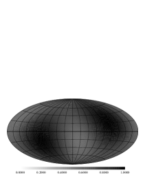
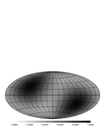
Figure 4: Maps of $f/f_{\rm max}$ in Aitoff-projected Galactic coordinates. The Galactic centre is at the centre of the maps; Galactic longitude increases from right to left. The real DMR data were used to produce the top panel; for the bottom panel, a large prominent hot spot, with an amplitude of 200$\,\mu$K and a $20^{\circ}$ radius, centred at $(l,b)=(45^{\circ},45^{\circ})$, was added to the data. The grey-scale runs from zero to one, so the low level of contrast in the top panel illustrates that $\cal D$ is not very large (i.e., that $f_{\rm min}/f_{\rm max}\equiv 1/{\cal D}$ is not very small).

4 Utility

Since the next generation of satellite experiments will produce extremely large (mega-pixel) data sets, it is important to devise statistical techniques that can be rapidly and efficiently calculated. This is an especially important concern in cases where the statistic has to be calibrated with Monte Carlo simulations. The statistic ${\cal D}$ described in this paper can be evaluated for an $N_{\rm p}$-pixel map with $O(N_{\rm p})$ calculations, which means that extensive Monte Carlo simulations will be possible even with mega-pixel maps.

The slowest step in the calculation of ${\cal D}$ is estimating the gradient map. Suppose the map has $N_{\rm p}$ pixels divided into $N_{\rm b}$ blocks, so that there are $M\equiv N_{\rm p}/N_{\rm b}$ pixels per block. Then each gradient estimate involves fitting a linear function to $M$ data points, at a cost of $O(M^{2})$ operations. The total operations count is therefore $O(M^{2}N_{\rm b})$, or $O(MN_{\rm p})$, with a prefactor of order unity. The appropriate value of $M$ in future experiments is unlikely to be much greater than the value $M=64$ used above: indeed, it may prove to be smaller, since future maps will have lower pixel noise than COBE. It should therefore be possible to estimate $\cal D$ with an operation count of order $100N_{\rm p}$. Even for data sets as large as those expected from MAP and Planck, it will be possible to calculate the statistic, and calibrate it with simulations, quite rapidly.

This statistic may also prove useful for sky maps at other wavelengths, such as x-ray and infrared maps. It can also be generalised to apply to maps of point sources by pixelizing the map in pixels large enough to contain many sources each. Thus it could be applied to galaxy or star catalogues which cover a sufficiently large solid angle.

The technique described in this paper can provide a valuable test for Galactic or zodiacal contamination in sky maps. Suppose we calculate $\cal D$ for a map from which such signals are supposed to have been removed. If $\cal D$ proves to be large, and if the maximum or minimum value of $f$ occurs in a direction close to the Galactic or ecliptic pole, then we would have good reason for suspecting residual contamination.

The $\cal D$ statistic can also naturally be applied to polarisation maps. In fact, the application to a polarisation map is even simpler than the technique described in this paper, since one can simply skip the initial gradient estimation and use the polarisation measurements themselves in place of the gradient estimates. (Note that the function $f$ depends quadratically on $\mn@boldsymbol{g}_{p}$, so the fact that a polarisation vector is defined only up to a sign does not matter.) Since the cosmic polarisation signals for MAP and Planck are expected to be rather weak, and the galactic signals fairly uncertain on large scales, the $\cal D$ statistic may prove useful in checking future polarisation maps for residual galactic contamination.

5 Conclusions

When the MAP and Planck satellites return their high-fidelity maps of the sky, they will be subjected to the full battery of available statistical tests. Specific patterns will be searched for, in order to constrain particular models, but there will also be general tests for patterns on the sky or general sorts of non-Gaussianity which might be present. Among those basic properties to search for, directionality is quite fundamental, and could be connected with various models for the structure of the Universe on the largest scales. We have discussed a general method for finding directionality, the $\cal D$ statistic, which requires no particular assumptions about the specific form of the directional pattern. This is a rather obvious statistic, being quadratic in the gradient of the temperature field, and with the only complication being the derivation of the appropriate weights to use when the map is not all-sky.

For polarisation maps, the application of the $\cal D$ statistic is even more straightforward, because the gradient does not have to be taken. And since the statistic is quite general, it could obviously be applied to maps at other wavelengths. For large-angle catalogues of discrete objects (e.g. x-ray clusters or radio galaxies) this statistic could also be utilised, after first extracting a smooth field from the catalogue. As well as providing constraints on tera-parsec scale exotica, there is a much more mundane use for the $\cal D$ statistic, namely testing for residual foreground or other systematic effects. For large maps our statistic will be particularly easy to apply, since it is straightforward and fast to calculate, a great advantage given the sizes of data set which are about to deluge us.

References

- [Barrow et al. 1997] Barrow J. D., Ferreira P. G., Silk, J., 1997, Phys. Rev. Lett., 78, 3610
- [Barrow, Juszkiewicz, & Sonoda 1985] Barrow, J. D., Juszkiewicz, R., & Sonoda, D. H., MNRAS, 213, 917
- [Bennett et al. 1996] Bennett C. L., et al., 1996, ApJ, 464, L1
- [Bond 1996] Bond J. R., 1996, in R. Schaeffer, ed., Les Houches Session LX, Theory and Observations of the Cosmic Background Radiation, Elsevier Science Press, p. 469
- [Bromley & Tegmark 1999] Bromley, B.C. & Tegmark, M., 1999, ApJ, 524, L79
- [Bunn et al. 1996] Bunn E. F., Ferreira P., Silk, J., 1996, Phys. Rev. Lett., 77, 2883
- [Bunn & White 1997] Bunn E. F., White M., 1997, ApJ, 480, 6
- [Carroll & Field 1997] Carroll S. M., Field G. B., 1997, Phys. Rev. Lett., 79, 2394
- [Cayón & Smoot 1995] Cayón, L. & Smoot, G., 1995, ApJ, 452, 487
- [Cornish et al. 1998] Cornish N. J., Spergel D. N., Starkman G. D., 1998, Phys. Rev., D57, 5982
- [de Oliveira-Costa et al. 1996] de Oliveira-Costa A., Smoot G. F., Starobinsky A., 1996, ApJ, 468, 457
- [Ferreira et al. 1998] Ferreira P. G., Magueijo J., Górski K. M., 1998, ApJ, 503, L1
- [Górski et al. 1996] Górski, K. M., et al., 1996, ApJ, 464, L11
- [Heavens 1998] Heavens, A. F. 1998, MNRAS, 299, 805
- [Hobson et al. 1998] Hobson M. P., Jones A. W., Lasenby A. N., 1998, submitted to MNRAS
- [Levin et al. 1997] Levin J., Barrow J. D., Bunn E. F., Silk J., 1997, Phys. Rev. Lett., 79, 974
- [Kogut et al. 1997] Kogut A., Hinshaw G., Banday A. J., 1997, Phys. Rev., D55, 1901
- [Lewin et al. 1999] Lewin A., Albrecht A., Magueijo J., 1999, MNRAS, 301, 131
- [Lineweaver et al. 1999] Lineweaver, C.H., Tenorio, L., Smoot, G.F., Keegstra, P., Banday, A.J.,& Lubin, P., 1996, ApJ, 470, 38
- [Magueijo 1995] Magueijo J., 1995, Phys. Rev., D52, 689
- [Novikov et al. 1999] Novikov D., Feldman H. A, Shandarin S. F., 1999, Int. J. Mod. Phys., D8, 291
- [Pando et al. 1998] Pando J., Valls-Gabaud D., Fang L.-Z., 1998, Phys. Rev. Lett., 81, 4568
- [Perivolaropoulos 1998] Perivolaropoulos L., 1998, Phys. Rev., D58, 103507
- [Smoot et al. 1992] Smoot G. F., et al., 1992, ApJ, 396, L1
- [Smoot & Scott 1998] Smoot G. F. & Scott D., 1998, in Caso C., et al., Eur. Phys. J., C3, 1, the Review of Particle Physics p.
- [Starobinsky 1993] Starobinsky A. A., 1993, JETP Lett., 57, 622
- [Souradeep et al. 1998] Souradeep T., Pogosyan D., Bond, J. R., 1998, in Tran Thanh Van, ed., Proc. XXXIII Recontres de Moriond, Fundamental Parameters in Cosmology, in press
- [Stevens et al. 1993] Stevens D., Scott D., Silk J., 1993, Phys. Rev. Lett., 71, 20
- [Tegmark & Bunn 1995] Tegmark, M. & Bunn, E.F. 1995, ApJ, 455, 1
- [Wandelt et al. 1998] Wandelt B. D., Hivon E., Górski K. M., 1998, in Tran Thanh Van, ed., Proc. XXXIII Recontres de Moriond, Fundamental Parameters in Cosmology, in press
- [White & Bunn 1995] White M., Bunn E. F., 1995, ApJ, 450, 477