On density and velocity fields and $\beta$
from the IRAS PSC$z$ survey

Abstract

We present a version of the Fourier Bessel method first introduced by Fisher, Lahav et al (1994) and Zaroubi et al (1995) with two extensions: (a) we amend the formalism to allow a generic galaxy weight which can be constant rather than the more conventional overweighting of galaxies at high distances, and (b) we correct for the masked zones by extrapolation of Fourier Bessel modes rather than by cloning from the galaxy distribution in neighbouring regions. We test the procedure extensively on $N$-body simulations and find that it gives generally unbiased results but that the reconstructed velocities tend to be overpredicted in high-density regions. Applying the formalism to the PSZ$z$ redshift catalog, we find that $\beta=0.7\pm 0.5$ from a comparison of the reconstructed Local Group velocity to the CMB dipole. From an anisotropy test of the velocity field, we find that $\beta=1$ CDM models models normalized to the current cluster abundance can be excluded with 90% confidence. The density and velocity fields reconstructed agree with the fields found by Branchini et al (1998) in most points. We find a back-infall into the Great Attractor region (Hydra-Centaurus region) but tests suggest that this may be an artifact. We identify all the major clusters in our density field and confirm the existence of some previously identified possible ones.

1 Introduction

Redshift surveys provide the only possibility for determining the three-dimensional density field of luminous matter which is crucial for studies of mass concentrations, the power spectrum, dynamical analyses to probe the relationship between dark and luminous matter and many other areas of observational cosmology. However, the relation between redshift space and real space, although given straightforwardly by Hubble’s law in the limit of large distances, is distorted on smaller scales by galaxy peculiar velocities (a full analysis of this was first given by Kaiser (1987)). Hence correcting for the distortions becomes the most important physical problem associated with redshift surveys. Several different types of these surveys are currently available, varying widely in their depth, sky coverage, and sampling density. Since this paper will be mainly concerned with analysis of the density and velocity fields, we use the recently completed PSC$z$ survey, which is ideal for our purposes because of its large number of galaxy redshift and its near-complete sky-coverage. Its depth is small enough to render effects of space curvature and galaxy evolution negligible in our calculations.

There are several methods of correcting for distortions to recover the real space density and velocity fields. These all use either linear theory or the Zel’dovich approximation, and are therefore ultimately very limited in their ability to reconstruct the high-density regions. They can roughly be separated into two types of methods:

Iterative methods: Since peculiar velocities are caused by gravitational acceleration, the velocity field can be recovered from the density field. Iterative methods use the redshift space density field to calculate a peculiar velocity field which can then be used to correct the density field distortions. The procedure is repeated until the velocity field converges – see Yahil, Strauss, et al (1991) and Kaiser, Efstathiou, Ellis et al (1991) for slightly different versions of this method.

Basis function methods: When transforming the measured redshift space density field into a combination of angular and radial basis functions, the distortion is concentrated in the radial part and its correction becomes an algebraic matrix problem. There are several different versions of this approach: Nusser and Davis (1991) transform the angular part into basis functions but express the radial part in differential equations which they then solve numerically. Their method uses the Zel’dovich approximation. Fisher, Lahav et al (1994) (FLHLZ in the following) and Zaroubi et al (1995) transform both angular and radial parts into basis functions, using a combination of spherical harmonics and spherical Bessel functions.

Other approaches include Kaiser and Stebbins (1991) and Saunders and Ballinger (1998).

Work on nonlinear corrections for the evolution of the power spectrum includes Peacock and Dodds (1994), Fisher and Nusser (1996), and Taylor and Hamilton (1996); a critical discussion of these may be found in Hatton and Cole (1998).

In this paper, we extend and apply the Fourier Bessel method which was first introduced by FLHLZ and Zaroubi et al (1995). Their treatment of dynamics using this expansion is new, but the idea of using spherical harmonics and even spherical Bessel functions goes back to Peebles (1973). It has been applied to redshift surveys by Scharf and Lahav (1993), Scharf, Hofmann, Lahav, Lynden-Bell (1992), and Fisher, Scharf and Lahav (1994). We will follow the original method closely but introduce two extensions:

• Conventionally, the weight given to each galaxy increases as the number density of galaxies decreases (as it does with radius in a flux-limited survey). We generalise the formalism to allow constant or any other weight, since we feel that care has to be taken with the conventional procedure: The purpose of this type of weighting is to exaggerate the mass of galaxies at higher radii where the sampling is poor, thereby making it possible to determine a density field. Note however, that since this also exaggerates the shot noise, the density field at high radii is subsequently considered unreliable and fluctuations are smoothed away.

• We correct for the mask by also using a basis function approach rather than the more usual cloning mechanism. The difference between these two methods is not an issue for IRAS-based surveys, which have very good sky coverage, but will be more interesting in the future with the advent of very deep surveys of small angular coverage such as the 2dF survey.

For our analysis, we use the recent PSC$z$ redshift survey. It contains approximately 15,500 galaxies (almost all) detected in the IRAS Point Source Catalog (Saunders (1996), Saunders et al (1998)) with 60 $\mu$m flux larger than 0.6 Jy. Our subsample contains 10549 PSC$z$ objects within 170 $\,h^{-1}{\rm Mpc}\$and with positive galaxy identification. Regions not surveyed by IRAS (two thin strips in ecliptic longitude and the area near the galactic plane defined by a V-band extinction of $>$ 1.5 mag) are excluded from the catalog which therefore covers $\sim$ 84 % of the sky.

The structure of the paper will be as follows: In section 2, we describe the correction for redshift space distortions using the Fourier-Bessel set of basis functions, and discuss the Wiener Filter smoothing procedure for suppressing shot noise. Details are given in the Appendices. In all of this, we mostly follow FLHLZ and Zaroubi et al (1995), but we have chosen to give derivations in full since we extended the original formalism and also changed some normalisations to render them more intuitive. In section 3 we present our method of correcting the masked areas. In section 4 we then test the method on $N$-body simulations to evaluate errors and systematic biases.

Sections 5, 6, and 7 present the analysis of the PSC$z$ redshift survey. In section 5, we recover $\beta$ from a comparison between the reconstructed velocity of the Local Group and its value known from the dipole anisotropy in the Cosmic Microwave Background (CMB). This procedure has a long tradition since the Local Group velocity is one of the few that is known accurately enough for a meaningful comparison to be made to its reconstructed value. However, the one-number-statistic nature of the procedure also makes it highly susceptible to systematic biases and we therefore take particular care to evaluate the error by analysing the scatter in the $N$-body simulations.

Section 6 analyses the magnitude of the redshift space distortions to recover another estimate of $\beta$ . It was first pointed out by Kaiser (1987) that the distortions themselves obviously depend on $\beta$ so that by analysing their magnitude, it should be possible to recover a value for that parameter. Several versions of such analyses have been done to date – ours relies on the fact that, if we correct the redshift space distortions assuming a wrong value for $\beta$ , the resulting density and velocity fields will be anisotropic, i.e., there will be a systematic difference between the radial and the other two directions. We develop a simple test for this anisotropy and estimate $\beta$ for the PSC$z$ again by comparing to the corresponding results for $N$-body simulations.

In section 7 we discuss the reconstructed density and velocity fields respectively and compare them to other recent reconstructions using the PSC$z$ and similar catalogs. Both of these fields result naturally from the reconstruction method we use if in a somewhat smoothed form due to the fact that our formalism only works in the linear regime.

2 The Fourier-Bessel method

The idea of this method is to express the overdensity as a Fourier-Bessel expansion

$$\delta(r,\hbox{\bmit\char 33\relax})=\sum_{lmn}Y_{lm}(\hbox{\bmit\char 33\relax})j_{l}(k_{ln}r)\delta_{lmn}.$$ (1)

Here ! denotes the angular coordinates, $Y_{lm}$ are spherical harmonics, $j_{l}$ are spherical Bessel functions, $k_{ln}$ are a set of wavenumbers that depend on the boundary conditions assumed, and $\delta_{lmn}$ are the expansion coefficients. Once the expansion coefficients are known,. the linear theory velocity field is easily calculated in terms of these, as

$${\bf v}(r,\hbox{\bmit\char 33\relax})=H_{0}\beta\sum_{lmn}\delta_{lmn}{\bf\nabla}\left(Y_{lm}(\hbox{\bmit\char 33\relax})\frac{j_{l}(k_{ln}r)}{k_{ln}^{2}}\right).$$ (2)

The problem is to determine the $\delta_{lmn}$ from redshift survey data, especially correcting for distortions of redshift space $(s,\hbox{\bmit\char 33\relax})$ relative to real space $(r,\hbox{\bmit\char 33\relax})$, arising from the velocity field. In this section we briefly describe how this is done, in the method introduced by FLHLZ, which we extend and apply in this paper. Full derivations are given in the Appendices.

2.1 Inverting redshift space distortions

From an all-sky redshift survey $(s_{i},\hbox{\bmit\char 33\relax}_{i})$, one can compute sums of the type

$$\rho^{S}_{lmn}=\sum_{s_{i}<R}w(s_{i})Y^{*}_{lm}(\hbox{\bmit\char 33\relax}_{i})j_{l}(k_{ln}s_{i}).$$ (3)

Here $w(s)$ is a weighting function for the galaxies, which we allow to be arbitrary. Now the $\rho^{S}_{lmn}$ seem like Fourier-Bessel expansion coefficients for the density field in redshift space (hence superscript $S$) but they depend on the selection function of the survey—denoted by $\phi(r)$—through the sum, as well as on $w(s)$. They are not the expansion coefficients unless $w(r)\phi(r)=1$. In linear theory the $\rho^{S}_{lmn}$ can be related to the sought-after $\delta_{lmn}$ by a messy but linear relation.

$${1\over\bar{\rho}}\sum_{n^{\prime}}(P_{l})^{-1}_{nn^{\prime}}\rho_{lmn^{\prime}}^{S,w}-O_{lmn}=\sum_{n^{\prime}}Z_{lnn^{\prime}}\delta_{lmn^{\prime}}^{Re}.$$ (4)

Here

$$O_{lmn}=\sqrt{4\pi}\int w\phi j_{0}(k_{ln}r)r^{2}dr$$ (5)

represents a monopole correction: initially we expand the density field. In order to transform to the overdensity field, we have to divide by the mean density $\bar{\rho}$ and subtract the $l=0$ (monopole) term from the coefficients. Note that the monopole correction does not really depend on $m$, but we have kept the index for consistency. The second step in equation 4 corrects the redshift space overdensity coefficients for the redshift space distortions expressed by

$$Z_{lnn^{\prime}} = \int w\phi j_{l}(k_{ln}r)j_{l}(k_{n^{\prime}}r)r^{2}dr$$ (6)

$$-\beta\int w\phi j_{l}(k_{ln}r)\left[\left(\frac{l(l+1)}{k_{n^{\prime}}^{2}r^{2}}-1\right)j_{l}(k_{n^{\prime}}r)+\frac{j_{l}^{\prime}(k_{n^{\prime}}r)}{k_{n^{\prime}}r}\frac{d\ln\phi}{d\ln r}\right]r^{2}dr.$$

The matrices

$$(P_{l})^{-1}_{nn^{\prime}}=\int w\phi j_{l}(k_{ln}r)j_{l}(k_{ln^{\prime}}r)r^{2}dr.$$ (7)

carry information about the weight function $w$.

Extracting $\delta_{lmn}$ from equation (4) involves solving a matrix equation for each $(l,m)$. $P_{lnn^{\prime}}$, $O_{lnn^{\prime}}$, and $Z_{lnn^{\prime}}$ depend on the weight function $w(r)$ and the selection function $\phi(r)$ but not on data.

The weight function $w(r)$ could be set to $1/\phi(r)$ to eliminate the selection function from the formulas. The correction matrices $P_{lnn^{\prime}}$ would then become diagonal and (7) would reduce to the orthogonality relation (A16) for spherical Bessel functions. The other extreme is to weight all galaxies equally $w(r)=1$, leaving the correction of the selection effect fully to the matrices $P_{lmn}$. The difference between these two approaches lies in the errors induced by shot noise. The choice $w(r)=1$ tends to extrapolate information from the well-sampled regions into less-sampled regions, while also propagating shot noise from less-sampled regions to well-sampled regions. The choice $w(r)=1/\phi(r)$ keeps the effect of shot noise more local. For the data set we have analyzed in this paper, the difference made by $w(r)$ is very small (see figure 4 below) indicating that the errors are nowhere dominated by shot noise. However, the situation is different when we encounter an analogous problem in Section 3. There the selection function is angular and becomes zero in the unobserved region; the information-propagation aspect then becomes crucial for filling in this region.

The expressions above are equivalent to FLHLZ but not identical because

• we have chosen to normalise the Fourier Bessel coefficients so that $F_{lmn}$ always have the same dimensions as $F(r,\hbox{\bmit\char 33\relax})$.

• our coefficients always refer to the Fourier Bessel basis set, whereas in FLHLZ they sometimes refer to an intermediate basis set that depends on the galaxy weight $w(r)$.

• we work entirely in the CMB rather than in the Local Group rest frame.

For this reason we have given full derivations in Appendix A.

2.2 Wiener Filter

A Fourier-Bessel expansion computed as above will contain spurious extra power from shot noise. This spurious power can be suppressed by a Wiener Filter as explained in Press et al (1992), p. 548, where the filter is

$$\Phi=\frac{\mbox{power in signal}}{\mbox{power in (signal + noise)}}.$$ (8)

The derivation of this expression, however, as given in Press et al (1992), is only valid for a scalar transfer function, whereas in our case the transfer function is $Z_{lnn^{\prime}}$. We will therefore have to derive our own Wiener Filter operator. The filter and its derivation are given in Appendix B, which mostly follows Zaroubi et al (1995). But we have presented the derivation in full since some of our normalizations are different and since we needed to preserve the arbitrariness in $w(r)$ throughout.

The Wiener Filter requires knowledge of the power spectrum $P(k)$ of the underlying density fluctuations. We do not know this in general, but since the filter is a correction, a first order error in the filter will only introduce a second order error in the full reconstruction (cf Press et al (1992), p. 548): even a fairly crude approximation of the power spectrum will make the filter work. We therefore use a CDM power spectrum with $\Gamma=0.4$, normalised to $\sigma_{8}=0.8$, as the filtering power spectrum for all our reconstructions. This resembles the spectrum fitted to data by Peacock and Dodds (1994) and all of the CDM spectra of the $N$-body simulations (see figure 1). A Wiener Filter on the basis of this power spectrum does as well in reconstructing velocities from simulated catalogs as a filter based on the power spectrum underlying the simulation in question. The advantage of using this constant filter rather than the ‘correct’ filter based on the underlying power spectrum is that the tests on the simulated catalogs will then accurately reflect the error introduced into the PSC$z$ reconstruction since we do not know the correct power spectrum in that case.

Figure 1 shows power spectra for several cosmologies, including our selected power spectrum and the one fitted to existing data by Peacock and Dodds (1994).

Figure 1: Power spectra for all models considered: SCDMC (standard CDM with $\Gamma=0.5$, $\sigma_{8}=1.1$, $\Omega=1.0$), SCDMG (standard CDM, COBE normalised with $\Gamma=0.25$, $\sigma_{8}=0.55$, $\Omega=1.0$), LCDM ($\Lambda$ CDM model with $\Gamma=0.25$, $\sigma_{8}=0.93$, $\Omega=0.3$, $\Lambda=0.7$), and PD94 (Peacock & Dodds, 1994), dashed line shows the power spectrum used for our filtering ($\Gamma=0.4$, $\sigma_{8}=0.8$)

3 Mask Correction

As mentioned above, the formalism developed in the preceding sections is only valid for a full-sky catalog. Most redshift surveys are masked in some way, so it is necessary to correct for the unobserved parts of the sky. This is done by introducing fake galaxies into the unobserved regions while trying to preserve the statistical properties of the galaxy distribution of the observed regions. The process is referred to as ‘mask correction’.

The usual method is to clone the fake from the observed galaxies by extrapolating the distribution from the observed into the unobserved regions. This works reasonably well, but has the following disadvantages:

• The joining-at-the-seams between the masked and unmasked regions has a tendency to introduce spurious power on some scales (since the correlation vanishes at the boundaries), which can contaminate the Fourier Bessel coefficients.

• The cloning method only works if the masked areas are very small compared to the unmasked areas. It is hopeless for redshift surveys with very small sky coverage such as the 2dF survey. It is therefore interesting to try out a Fourier Bessel based mask correction here for possible application with that survey. Naturally, with small sky coverage, only high-$l$ modes might be usefully constrained, but this may still extract information about density and velocity fields on scales smaller than the survey.

As mentioned in section A.3, it is in principle possible to treat the angular window function $\varphi(\hbox{\bmit\char 33\relax})$ at the same time as the selection function $\phi(r)$ but it is computationally problematic. We therefore choose to correct in two steps: we first treat the mask and then the selection function. To this end, we have to first expand the density field in such a way as to decouple the angular modes completely from the radial modes. Let $\varrho(s,\hbox{\bmit\char 33\relax})$ be the ‘raw’ redshift space density, i.e.,

$$\varrho(s,\hbox{\bmit\char 33\relax})=\phi(r)\rho^{S}({\bf s}),$$ (9)

separate the angular and radial parts and expand

$$\varrho(s,\hbox{\bmit\char 33\relax})=\sum_{lmn}\varrho_{lmn}Y_{lm}(\hbox{\bmit\char 33\relax})j_{0}(k_{0n}s).$$ (10)

Note that because only $j_{0}$ occurs in this expression, the radial and angular basis functions are truly independent and are not eigenfunctions of the Laplacian operator. They do, however, form an adequate description of the density field for the purpose of correcting for the angular mask.

We minimise

$$\int\varphi(\hbox{\bmit\char 33\relax})\left|\varrho(s,\hbox{\bmit\char 33\relax})-\sum_{lmn}\varrho_{lmn}Y_{lm}(\hbox{\bmit\char 33\relax})j_{0}(k_{0n}s)\right|^{2}d\hbox{\bmit\char 33\relax}s^{2}ds$$ (11)

to obtain

$$\int\varphi(\hbox{\bmit\char 33\relax})Y^{*}_{lm}j_{0}(k_{0n}s)d\hbox{\bmit\char 33\relax}s^{2}ds=C^{-1}_{0n}\sum_{ll^{\prime}mm^{\prime}}\varrho_{l^{\prime}m^{\prime}n}\int\varphi(\hbox{\bmit\char 33\relax})Y_{l^{\prime}m^{\prime}}(\hbox{\bmit\char 33\relax})Y^{*}_{lm}(\hbox{\bmit\char 33\relax})d\hbox{\bmit\char 33\relax}.$$ (12)

The integrals can be replaced by sums over galaxies as before. We invert the matrix on the right hand side and thereby recover $\varrho_{lmn}$ and hence $\varrho(s,\hbox{\bmit\char 33\relax})$. This recovered density field can then be sampled in the masked regions to provide the fake galaxies.

As an additional way of minimising the errors in this procedure, we invert the matrix with a conditioned inversion, i.e., after diagonalising we note all those eigenvalues which are less than 1 % of the largest eigenvalue and eliminate the corresponding eigensubspaces. The eigenvalues of the matrix will be unity for unmasked modes and small for mostly masked modes. Hence, the noise can be suppressed by suppressing the masked modes. The procedure is similar to applying a Wiener Filter and ensures that the density field is not dominated by spurious features in the masked zones.

Figure 2 shows a slice of the masked and unmasked galaxies in the $x$-$z$ plane.

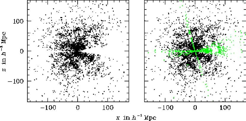
Figure 2: Projections of galaxy positions onto a plane in $x$-$z$ (where the $x$-axis points towards $l=0^{\circ}$ and the $z$-axis towards $b=90^{\circ}$; $y\mbox{ }\epsilon\mbox{ }[-20,20]$); unfilled and filled masked zones; Note how the mask correction produces voids around (70,0) and (-20,50) which appears to be extrapolations of voids in the surrounding data.

4 Tests on Simulated Catalogs

The method described above can now be tested on simulated catalogs with known selection function $\phi(r)$. We reconstruct the real space density and velocity fields as described above and then sample it at the real space galaxy positions. The $r_{i}$ of each galaxy is reconstructed from its $s_{i}$ and the radial velocity field (cf equation A23) by Newton-Raphson iteration. Reconstruction is done for a radius $R$ of 170 $\,h^{-1}{\rm Mpc}\$and a minimum radial resolution $r_{\rm min}$ of 5 $\,h^{-1}{\rm Mpc}\$. Our galaxy weight is given by $w(r)=1/\phi(r)$. We will use this to be more in line with standard procedure in all of the following reconstructions unless otherwise stated.

Figure 3 shows a comparison of real against predicted velocities in the $r,\theta,\phi$ directions for an LCDM catalog (for the parameters relating to the model abbreviations LCDM, SCDMC, and SCDMG see the caption of 1). The solid line is the line of perfect correlation and the dashed line represents a fit to the data. Note that this is not a fit in the least squares sense. We found that least squares fits have the tendency to be too easily dominated by outliers and therefore devised a more stable fitting routine (see also the discussion in Press et al (1992), p. 700). We constrain the fitted line to pass through the origin and choose the slope to be such that if we were to rotate the line by $90^{\circ}$ it would cross exactly half the points. This does not ignore the outliers but it only accounts for their numbers rather than for their distance to the line.

The figure illustrates that most of the error in the reconstruction lies in the $r$ direction, as would be expected since the redshift space distortions reside exclusively in that dimension. The error in the $\theta$ and $\phi$ directions is produced by shot noise only. In the following we will here only plot the radial velocity comparisons, since they are the most interesting in assessing the performance of the method. Note also that the reconstruction was performed using a ‘constant filter’, i.e., instead of using the correct power spectrum for this cosmology, we used the chosen power spectrum discussed in section 2.2.

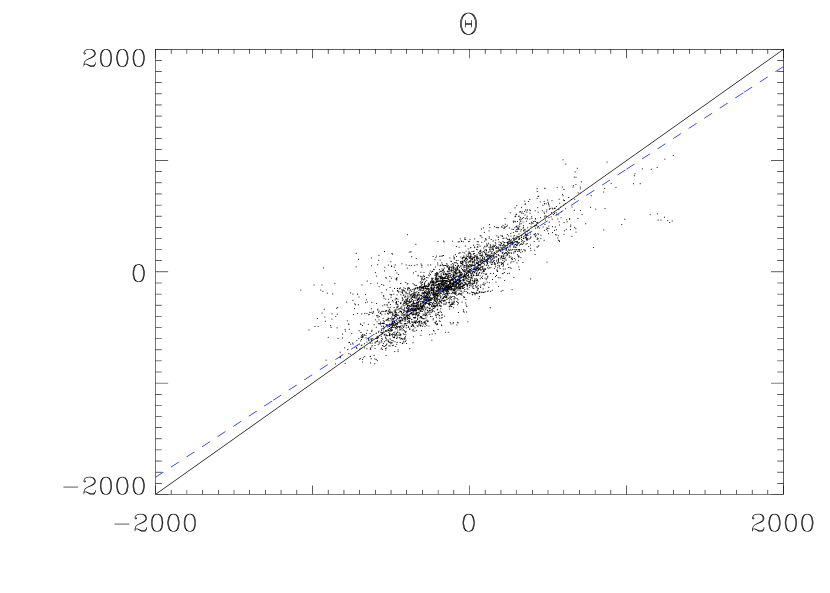
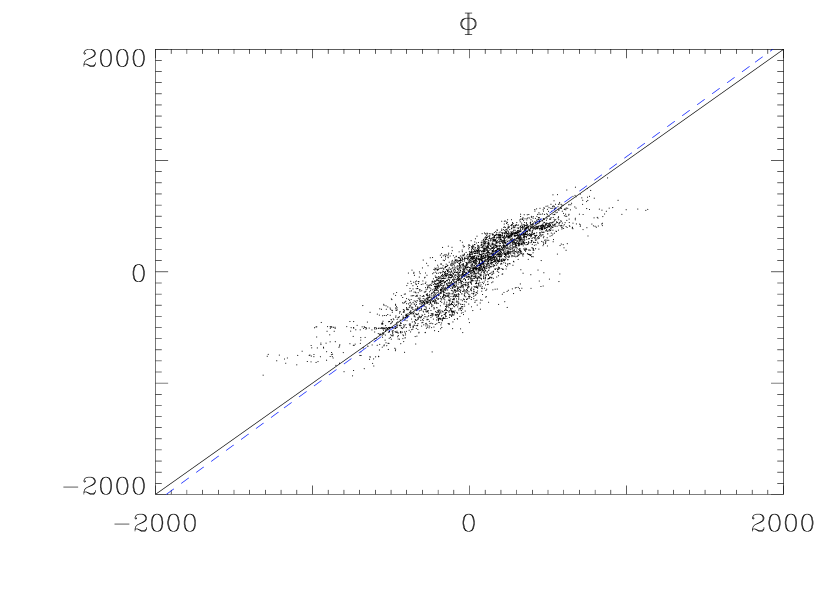
Figure 3: Real (vertical) against reconstructed (horizontal) velocities: $v_{r},v_{\theta},v_{\phi}$ for an LCDM catalog; plot galaxies out to 60 $\,h^{-1}{\rm Mpc}\$, $1/\phi$ weighting, constant filter; it is obvious that the maximum error is in $v_{r}$.

Figure 4 shows the effect of using different types of filter. The first panel shows a reconstruction for an LCDM catalog using no filter. The second panel shows the same catalog, but in this case the velocities were reconstructed with the constant filter. The variance is smaller now since most of the shot noise is smoothed away. The third panel shows exactly the same case but we have here used a constant weighting function $w(r)=1$. The result illustrates that in the case of the velocity reconstruction the results are the same whether we use an inverse selection function or a constant weighting for each galaxy.

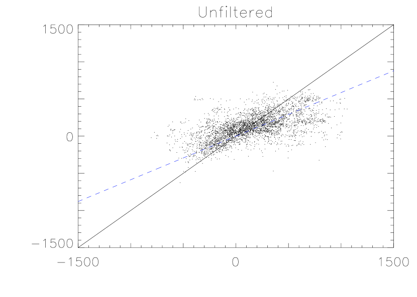
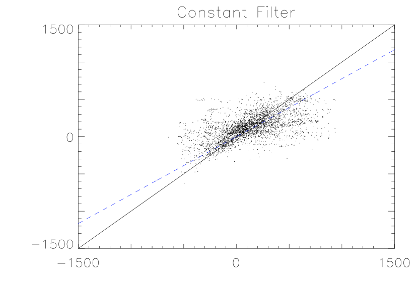
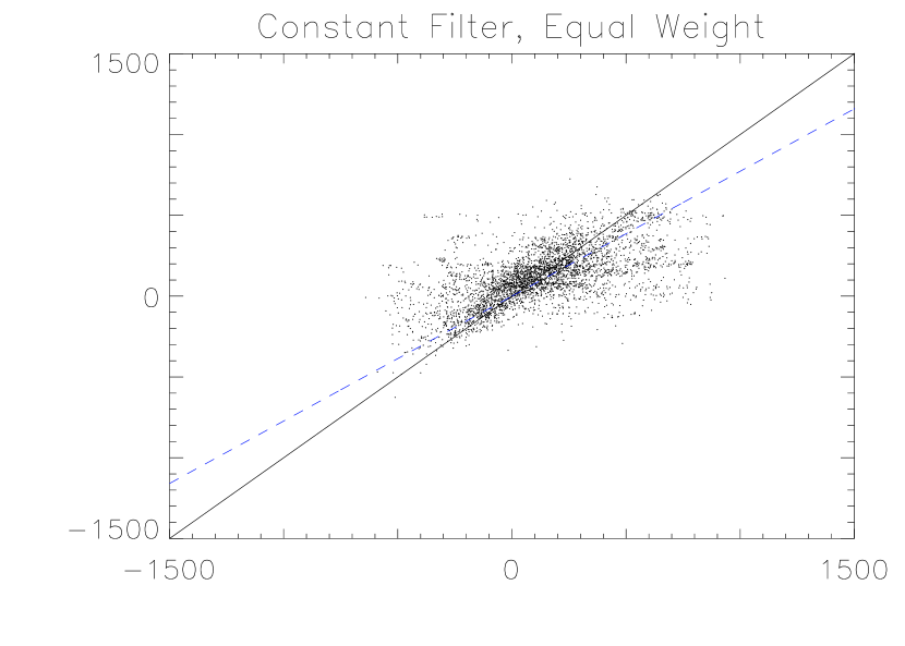
Figure 4: Real against predicted velocities for three different types of filters; LCDM catalog; plot galaxies out to 60 $\,h^{-1}{\rm Mpc}\$, $1/\phi$ weighting in all but the last panel.

Figure 5 shows the real against predicted radial velocities for one catalog of each cosmology using a constant filter reconstruction.

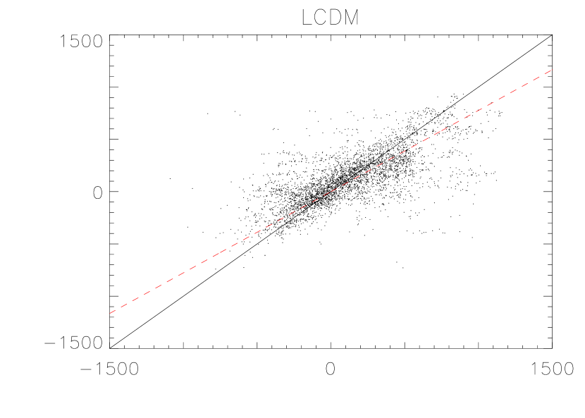
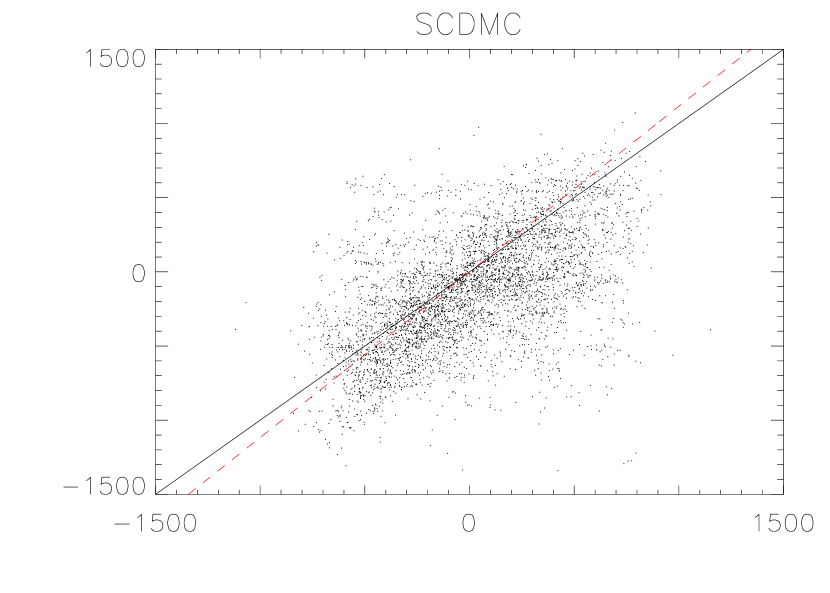
Figure 5: Real against predicted velocities for three different cosmologies; one catalog for each cosmology; plot galaxies out to 60 $\,h^{-1}{\rm Mpc}\$.

Table 1 shows the results of applying our line fitting to the constant filter reconstructions. The parameter $B$ is the slope of the line averaged over all 10 catalogs in a given cosmology, and $d$ is the average distance of a point from the line.

LCDM Results
Case	$B\pm\sigma_{B}$	$d\pm\sigma_{d}$
$r<120$	0.92 $\pm$ 0.08	244 $\pm$ 25
$r<60$	0.80 $\pm$ 0.07	220 $\pm$ 31
$60<r<120$	1.14 $\pm$ 0.22	270 $\pm$ 35
$\delta<1$	1.17 $\pm$ 0.15	233 $\pm$ 25
$\delta>1$	0.76 $\pm$ 0.34	288 $\pm$ 67
$-1<\delta<1$, $r<60$	0.95 $\pm$ 0.07	184 $\pm$ 24
SCDMG Results
$r<120$	0.90 $\pm$ 0.07	224 $\pm$ 26
$r<60$	0.82 $\pm$ 0.07	212 $\pm$ 29
$60<r<120$	1.05 $\pm$ 0.19	241 $\pm$ 40
$\delta<1$	0.99 $\pm$ 0.08	232 $\pm$ 23
$\delta>1$	0.74 $\pm$ 0.18	278 $\pm$ 52
$-1<\delta<1$, $r<60$	0.85 $\pm$ 0.07	193 $\pm$ 27
SCDMC Results
$r<120$	1.01 $\pm$ 0.11	457 $\pm$ 49
$r<60$	0.84 $\pm$ 0.12	407 $\pm$ 71
$60<r<120$	1.27 $\pm$ 0.13	517 $\pm$ 28
$\delta<1$	1.17 $\pm$ 0.16	467 $\pm$ 28
$\delta>1$	1.37 $\pm$ 1.51	751 $\pm$ 685
$-1<\delta<1$, $r<60$	0.92 $\pm$ 0.15	372 $\pm$ 77

Table 1: Parameters of fitted line and velocity dispersions for three different cosmologies and 6 different cases. All distances are in $\,h^{-1}{\rm Mpc}\$. $B$ is the slope of the fitted line, $\sigma_{B}$ the dispersion in the average over all 10 catalogs, d is the average distance of a point from the fitted line and $\sigma_{d}$ its dispersion.

A high-density selection in the Fourier Bessel case is more damaging to the correlation than a high-radius selection. Note that in the worst possible cosmology (SCDMC), the correlation practically ceases in the high density case but is comparatively normal (by the standards of that universe) for the high radius case. For all cosmologies, there is a clear tendency to overpredict velocities in high density regions.

Figure 6 again illustrates the dependence of reconstruction error on local density: for the same representative reconstructions for each cosmology as in figure 5, we plot the reconstructed density field (contours) and the difference between the reconstructed and the real velocity field (arrows).

Figure 6: $\Delta v=v_{\rm pred}-v_{\rm real}$ for three different cosmologies (same catalogs as before); Density levels indicate overdense regions only, bold line is at $\delta=0$ and the contours are evenly spaced in 13 steps from $\delta=1$ to $\delta=7$. Velocity vectors are drawn on an arbitrary scale.

The differences are most marked in the SCDMC case and in all three cases, there is a clear correlation of velocity error with overdensity. Since the arrows point towards the overdensities, the infall into clusters is overpredicted.

To test the dependence on radius, we also plot the velocity difference for the SCDMC case out to 170 $\,h^{-1}{\rm Mpc}\$(figure 7). Note that there is no indication that the greater shot noise at high radii produces a systematic effect. Even in those regions, the errors caused by overdense regions far outweigh any radius dependence. Again, this is a trend already indicated in table 1.

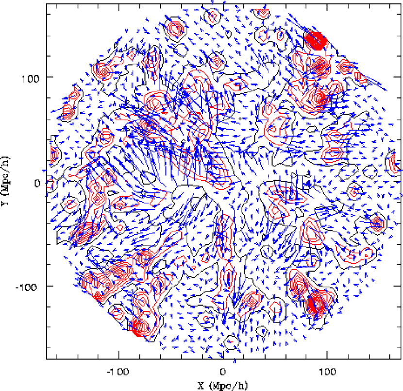
Figure 7: $\Delta v=v_{\rm pred}-v_{\rm real}$ for SCDMC; density levels indicate overdense regions only, bold line is at $\delta=0$, thin lines are overdensities from $\delta=2$ to $\delta=32$ in 16 steps; the smallest velocity difference for this plane is 18 km s^-1and the largest 1788 km s^-1.

5 Local Group Velocity and $\beta$

The velocity field reconstructed by the above method is of particular interest at the origin: by comparing the reconstructed velocity, ${\bf v}(0)$, of the Local Group (LG) to the Local Group velocity, ${\bf v}_{LG}$, measured from the dipole in the CMB we can recover $\beta$ .

Since only the dipole contributes to the velocity ${\bf v}(0)$ (cf equation A30), we can set $l_{\rm max}=1$ for this particular calculation. We also increase $r_{\rm min}$ to 10 $\,h^{-1}{\rm Mpc}\$to increase the stability of the reconstructed LG velocity. If the resolution is too high, the calculated velocity tends to be too easily influenced by small but nearby density fluctuations.

Figure 8 shows the measured LG velocity amplitudes for reconstructions using $\beta$ = 0.3 to 1.0 (steps of 0.1) rescaled to $\beta$ = 1. We plot this against the angle between the reconstructed LG velocity direction and the CMB dipole direction (misalignment angle).

Figure 8: Dipole amplitude and misalignment against different $r_{\rm max}$ for the PSC$z$; note that the velocity is rescaled to $\beta$ = 1 in the upper panel.

Note that the reconstructed velocity does not seem overly sensitive to the $\beta$ assumed in the reconstruction. The rescaled amplitudes are all in the range between 1000 km s^-1and 1100 km s^-1and hence we can conclude that $\beta\simeq 0.7$. The very good alignment between the reconstructed velocity and the CMB dipole indicates that we are satisfactorily sampling the matter that causes the acceleration. Note also that the convergence of the dipole amplitude is very good. The Fourier Bessel method works entirely in the CMB frame and we therefore do not have any signature from the Kaiser rocket effect (discussed, for example, in Strauss et al (1992)).

Instead of performing a likelihood analysis, in this case we evaluate systematic effects by calculating the LG velocity for all 30 catalogs to look at the scatter in

$$({\bf v}(0)-{\bf v}_{LG})^{2}.$$ (13)

We render this dimensionless and define

$$\mu^{2}=\left(\left(\frac{v}{v_{LG}}\right)^{2}-2\cos\vartheta\frac{v}{v_{LG}}+1\right),$$ (14)

where $\vartheta$ is the misalignment angle. This method may be less sophisticated than a likelihood analysis (e.g., Schmoldt, et al (1998)) but it makes fewer assumptions about the underlying cosmology. It works on the simple basis of comparing real data against results from simulated catalogs.

Figure 9 plots the quantity $v/v_{LG}$ against the misalignment angle for all simulated catalogs and the PSC$z$ together with contour lines of the surface equation 14. The LG velocity for the PSC$z$ was reconstructed using $\beta=0.7$ as was indicated by the above result. The inner contour encloses 2/3 of the simulation points and hence it defines our 68 % confidence limits on $\beta$ . Therefore, we recover $\beta=0.7\pm 0.5$. This result seems a lot less restrictive than the one quoted in Schmoldt, et al (1998) but it has to be noted that in that work the results separate the high and low normalisation cases. In this case, we consider all simulations at the same time – drawing together the two different values for $\beta$ in Schmoldt, et al (1998) would give a similarly ill-constrained result.

Figure 9: Dipole determinations for all catalogs: triangle = PSC$z$, + = SCDMC, * = SCDMG, square = LCDM.

It is interesting to note that most of the velocity ratios are close to unity but that the misalignment angle can get quite large. This is particularly the case for the SCDMC catalogs, which are (as already mentioned) dominated by large fluctuations at small radii. This seems to affect the misalignment much more than it does the amplitude.

6 Velocity Anisotropy and $\beta$

The density field $\delta^{Re}$ should in general be perfectly isotropic, i.e., there should be nothing special about the radial direction. The radial redshift space distortions in the density field $\delta^{S}$, however, depend on $\beta$ so that $\beta$ can in principle be recovered from analysing those distortions.

We recover the full $\delta^{Re}$ in our method, and if we do so with the correct $\beta$ , the density field should be isotropic. Therefore, we simply devise an anisotropy test which will detect radial anisotropies caused by a reconstruction of the density field using the wrong $\beta$ . Note that this method tests reconstructed real space velocities and not the redshift space density field. In order to avoid problems caused by a small sample (i.e., in order to improve the chance that the normal anisotropies will average out in the volume considered) we restrict the analysis to regions where $\delta<1$.

Increasing $\beta$ in $Z_{lnn^{\prime}}$ (in equation 4) suppresses structure in the radial direction (since the redshift space distortions create such structure artificially). If our assumed $\beta$ is too high, then the recovered $v_{r}$ will be too low. We therefore define the parameter

$$\eta=\frac{1}{3}\frac{\langle{\bf v}^{2}\rangle-\langle{\bf v}\rangle^{2}}{\langle v_{r}^{2}\rangle-\langle v_{r}\rangle^{2}},$$ (15)

where the averages are weighted by the local density $(1+\delta)$. We expect $\eta$ to pass through unity at the correct $\beta$ .

To calculate the value of $\eta$ for different catalog reconstructions, we sample the velocity field in a radius of 60 $\,h^{-1}{\rm Mpc}\$of the origin with a collection of 800 random points having $\delta<1$. (We exclude regions with $\delta>1$ since our reconstructions have larger errors there.) In figure 10, we plot $\eta$ against various trial $\beta$ for 10 SCDMG and 10 LCDM catalogs. We have discounted the SCDMC catalogs for this test because of their unrealistically large density fluctuations on small scales (much larger than observed clustering) and partly because of the high variance in the predicted velocities (see table 1). An anisotropy test on SCDMC would be too noisy to give useful results.

In general, the scatter is too large for a clear statement about the $\beta$ at which the lines cross unity. However, we can recognise some trends. Generally, the SCDMG points ($\beta$ = 1) are lower, i.e., they cross unity later than the LCDM points ($\beta$ = 0.5) as would be expected. This suggests treating $\eta$ as a statistic, and the values obtained from the 10 SCDMG and 10 LCDM catalogs as samples of the distribution of $\eta$ in the respective cosmologies. We find (cf 10) that, for all trial $\beta$ , the value of $\eta$ from PSC$z$ exceeds at least 9 (usually all 10) of the values from PSC$z$. This is not the case for LCDM. We therefore conclude that SCDM is excluded at the 90% confidence level.

It is worth noting that not all $\beta$ =1 models can be rejected on the basis of this result, since models with more large-scale power will also have more cosmic variance, increasing the scatter in $\eta$.

Figure 10: Plot of $\eta$ for different trial $\beta$ from PSC$z$, and from 10 SCDM and 10 LCDM catalogs. The PSC$z$ line lies among the LCDM values but is almost completely disjoint from the SCDMG values.

7 Local Density and Peculiar Velocity Fields

Figures 11 and 12 show the PSC$z$ velocity and density field in the supergalactic plane out to 70 and 170 $\,h^{-1}{\rm Mpc}\$respectively. The general features agree very well with the velocity field reconstructed in Branchini et al (1998). We recover the same continuous flow from the northern end of the Perseus-Pisces cluster to the GA region. However, we also find a back-infall into this region, which was not observed in Branchini et al (1998). This is more apparent in figure 12: there is a clear division between the back-infall into Hydra-Centaurus and the subsequent infall into the Shapley cluster (-100,90). The highest velocity for any of the back-infalling galaxies is 494 km s^-1and therefore above the dispersion level given in table 1. However, table 1 also indicates that the infall into high density regions will in general be overpredicted. Likewise, comparing the real and predicted velocity maps of the simulated catalogs, we find that the overpredicted infall makes for a more sharply peaked velocity field in the reconstructions and hence in about half of the maps for the SCDMG catalogs, for example, it is easy to identify regions where the reconstructions show a back-infall into a cluster that does not exist in the real velocity field. We cannot therefore consider the evidence conclusive.

Figure 11: Velocity field of the PSC$z$ survey: radius out to 70 $\,h^{-1}{\rm Mpc}\$. Contour lines denote density field (fat line = zero density contrast, broken lines = underdensities, thin solid lines = overdensities).

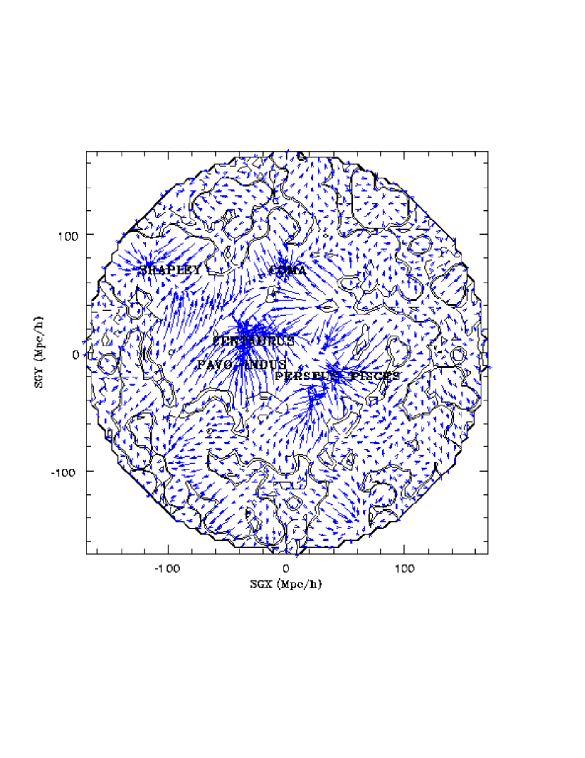
Figure 12: Velocity field of the PSC$z$ survey: radius out to 170 $\,h^{-1}{\rm Mpc}\$.

Figure 13 presents the PSC$z$ density field. We have plotted all those galaxies, for which the local density $\delta({\bf r})$ as determined from the density coefficients is higher than the threshold $\delta=1.0$ and which are within a radius of 130 $\,h^{-1}{\rm Mpc}\$of the observer.

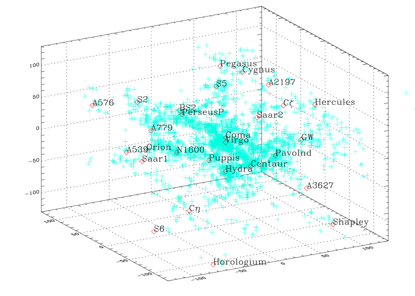
Figure 13: Clusters in the PSC$z$ survey: Density level at 1.0.

We labelled all the known superclusters as before. The same structures are identified and it is particularly interesting to note the extension to Hydra.

8 Conclusions

We have corrected the redshift space distortions in the PSC$z$ survey via the Fourier-Bessel method of FLHLZ with two extensions: a generic galaxy weight and a matrix correction for the masked zones. The method was tested extensively on mock catalogs extracted from $N$-body simulations. It was shown not to have any systematic biases except for an overprediction of velocities in high density regions. We find

• an LG velocity that well reproduces the CMB dipole for $\beta$ = 0.7. We estimate the error on this value from the scatter in the simulations as $\pm$ 0.5.

• that an $\Omega=1.$, cluster normalised and standard CDM cosmology is ruled out with a confidence of 90 % from a new anisotropy test.

• a flow field in the supergalactic plane that is consistent with the results of Branchini et al (1998) apart from an observed back-infall into the Hydra-Centaurus region. However, we treat this result with caution since the simulations show spurious features of this type.

• a density field that shows all the usual clusters and confirms two of the ones identified by Webster, Lahav, and Fisher (1997). There is a possible conincidence of Saar2, a structure identified in the PSC$z$ by Saar (1996), and the C$\zeta$ cluster of Webster, Lahav, and Fisher (1997) and likewise of Saar1 with the Orion and A539 clusters. We also confirm the existence of A3627 and identify an extension to the Hydra-Centaurus supercluster.

Appendix A Dynamical Theory

This appendix derives the equations in section 2 that express the express the real-space overdensity and velocity fields under linear theory from survey data via a Fourier Bessel expansion.

We will first introduce the mathematics associated with the distortion correction. These are independent of the choice of basis functions so it is only after the derivation that we motivate our particular set of functions (spherical harmonics and spherical Bessel functions) by the observation that they are eigenfunctions of the Laplacian operator and therefore render the velocity calculations particularly easy. We then present the form of the distortion correction for this basis function set.

A.1 Redshift Space Distortions

The transformation between redshift space ${\bf s}$ and real space ${\bf r}$ is given by

$${\bf s}={\bf r}+\hbox{\bmit\char 33\relax}u({\bf r}),$$ (A1)

where $u({\bf r})$ is the radial peculiar velocity at a point ${\bf r}$ and ! is the angular unit vector, i.e., $\hbox{\bmit\char 33\relax}=\hat{{\bf r}}$.

Consider some function $f({\bf s})$ of the galaxy positions ${\bf s}$ in redshift space given by a survey. Summing over that function at the galaxy positions will be equal to the integral over all space of the function multiplied with the the sampling function of the galaxies, i.e.,

$$\sum_{s_{i}<R}f({\bf s}_{i})=\int_{4\pi}d\hbox{\bmit\char 33\relax}\int_{0}^{R}f(s,\hbox{\bmit\char 33\relax})\rho^{S}(s,\hbox{\bmit\char 33\relax})\phi(r)s^{2}ds,$$ (A2)

where $\rho^{S}(s,\hbox{\bmit\char 33\relax})$ is the redshift space density field, $\phi(r)$ is the selection function (note that it depends on $r$, not $s$, since a galaxy’s inclusion into a flux-limited survey depends on its position in real space) and $R$ is the maximum radius of the survey in redshift space. To a zeroth order approximation, this sum will be equal in redshift and in real space. In the following, we will work out a first order correction to that approximation by finding the analogous sum in real space.

We now hold ! constant since the effect of redshift space distortions is isolated in the radial component. Mass conservation requires that

$$\rho^{S}(s)s^{2}ds=\rho^{Re}(r)r^{2}dr,$$ (A3)

where $\rho^{Re}$ is the real space density field, so we can rewrite the right hand side of equation A2

$$\int_{0}^{R}f(s)\phi(r)\rho^{S}(s)s^{2}ds=\int_{0}^{R-u}f(s)\phi(r)\rho^{Re}(r)r^{2}dr.$$ (A4)

Note that the boundaries on the integrals have changed. The maximum radius $R$ is defined in redshift space and therefore also has to be transformed to real space. We then expand $f(s)$ in a Taylor series of the form

$$f(r+u(r))=f(r)+uf^{\prime}(r)+\ldots$$ (A5)

and drop all second order terms, so that

$$\int_{0}^{R}f(s)\rho^{S}(s)\phi(r)s^{2}ds=\int_{0}^{R-u}f(r)\rho^{Re}(r)\phi(r)r^{2}dr+\int_{0}^{R-u}uf^{\prime}(r)\rho^{Re}(r)\phi(r)r^{2}dr.$$ (A6)

The first integral on the right hand side has to be split into two parts

$$\int_{0}^{R-u}f\phi\rho^{Re}r^{2}dr=\int_{0}^{R}f\phi\rho^{Re}r^{2}dr+\int_{R}^{R-u}f\phi\rho^{Re}r^{2}dr$$ (A7)

since it is a zeroth-order term and the integral between $R$ and $(R-u)$ cannot be neglected (note that we have ceased to give the dependence on $r$ in all the functions to make the equations neater). The last term in equation A7 is first-order, so we can replace $\rho^{Re}$ by its average value $\bar{\rho}$, multiply the integrand with $u$, and evaluate the functions at $R$.

The second integral in equation A6 is a first-order term, so we can again replace $\rho^{Re}$ by $\bar{\rho}$ and integrate by parts. Simplifying, we get

$$\int_{0}^{R}f(s)\rho^{S}(s)\phi(r)s^{2}ds=\int_{0}^{R}f\phi\rho^{Re}r^{2}dr-\bar{\rho}\int_{0}^{R}f\frac{d}{dr}\left(u\phi r^{2}\right)dr$$ (A8)

Here the first term is the real space expression (analogue of the redshift space sum in equation A2) that we were looking for and the second term represents the redshift space distortions. We can gain some insight into the nature of these distortions by rewriting this term as

$$\bar{\rho}\int_{0}^{R}f\phi r^{2}\left[u^{\prime}+\left(\frac{d\ln\phi}{d\ln r}+2\right)\frac{u}{r}\right]dr,$$ (A9)

where the terms in the square brackets now describe the various contributions to the distortions, i.e.,

• the galaxies’ peculiar velocities: the velocity field at a real space position ${\bf r}$ will be different from the field at ${\bf s}$ – hence the $u^{\prime}$ term.

• the selection function: there is a change in the selection function between $r$ and $s$ – hence the $d\ln\phi/d\ln r$ term.

• the volume change: a shell at $r$ has a different volume from a shell at $s$ – hence the $2u/r$ term.

These were first pointed out by Kaiser (1987). Note that of the two kinds of redshift space distortion discussed in that paper, this expression only treats the second, linear kind and hence a redshift space correction on the basis of this expression will only work in the linear regime.

Now, putting back the !-dependence, we have

$$\sum_{s_{i}<R}f({\bf s}_{i})=\int d\hbox{\bmit\char 33\relax}\left[\int_{0}^{R}f(r,\hbox{\bmit\char 33\relax})\phi(r)\rho^{Re}(r,\hbox{\bmit\char 33\relax})r^{2}dr-\right.$$

$$\left.\bar{\rho}\int_{0}^{R}f(r,\hbox{\bmit\char 33\relax})\frac{\partial}{\partial r}\left(u(r,\hbox{\bmit\char 33\relax})\phi(r)r^{2}\right)dr.\right]$$ (A10)

This represents the general equation for the correction of the redshift space distortions. We shall find a more specific expression after deciding on the form of $f$.

A.2 Peculiar Velocities

In linear theory, the velocity is the gradient of the gravitational potential (see Peebles (1993), p. 116)

$${\bf v}=-\frac{2}{3}\frac{f(\Omega_{0})}{\Omega_{0}H_{0}}\nabla\psi.$$ (A11)

Note that ${\bf v}$ is, as usual, a comoving peculiar velocity at the present time of which $u$ in equation A1 is the radial part. Poisson’s equation states that

$$\nabla^{2}\psi=\frac{3}{2}\Omega_{0}\delta_{\rm matter}H_{0}^{2}.$$ (A12)

We use the standard approximation $f(\Omega_{0})\simeq\Omega_{0}^{0.6}$, convert the density contrast $\delta_{\rm matter}$ to the galaxy density contrast $\delta$, assuming constant bias. The velocity therefore becomes

$${\bf v}=H_{0}\beta{\bf\nabla}(\nabla^{-2}\delta),$$ (A13)

A.3 Fourier Bessel Expansion

Since peculiar velocities are our main interest, we want to render the solution of equation A13 as easy as possible. It is obvious that the calculation of ${\bf v}$ will be trivial if we can find an expansion for $\delta$ that is an eigenfunction of the Laplacian operator. We also require the expansion to be in spherical coordinates : firstly because a separation of the angular and radial parts will concentrate the redshift space distortions in only one dimension, but also because the decreasing selection function of a redshift survey will tend to render its volume spherical. We therefore choose the Fourier Bessel expansion

$$F(r,\hbox{\bmit\char 33\relax})=\sum_{lm}F_{lm}(k)Y_{lm}(\hbox{\bmit\char 33\relax})\int j_{l}(kr)dk.$$ (A14)

Since the volume of the redshift survey is finite, we approximate the integral on the right hand side by the sum

$$F(r,\hbox{\bmit\char 33\relax})=\sum_{lmn}F_{lmn}Y_{lm}(\hbox{\bmit\char 33\relax})j_{l}(k_{ln}r),$$ (A15)

i.e., we confine ourselves to $k$-values satisfying certain boundary conditions on the survey range $R$. There will then be an orthogonality relation

$$\int_{0}^{R}j_{l}(k_{ln}r)j_{l}(k_{ln^{\prime}}r)r^{2}dr=\delta^{K}_{nn^{\prime}}C^{-1}_{ln},$$ (A16)

where $\delta^{K}$ denotes a Kronecker $\delta$. The $Y_{lm}(\hbox{\bmit\char 33\relax})$ are of course orthonormal. The values of $C_{ln}$ and $k_{ln}$ depend on the precise boundary conditions. We follow one common choice, which is to require $\delta=0$ at $r>R$ with $\delta$ allowed to be discontinous at $r=R$, but the logarithmic derivative of the gravitational potential $d\ln\psi/d\ln r$ required to be continous at that boundary. In this case,

$$k_{ln}\mbox{ are zeroes of }j_{l-1}(kR)$$ (A17)

$$C_{ln}^{-1}=\frac{1}{2}R^{3}\left(j_{l}(k_{ln}R)\right)^{2}.$$ (A18)

For a discussion of other possible boundary conditions see FLHLZ, appendix A.

If $F({\bf r})$ was known everywhere, we could simply invert equation A15 using orthogonality to obtain

$$F_{lmn}=C_{ln}\int_{V_{R}}Y^{*}_{lmn}(\hbox{\bmit\char 33\relax})j_{l}(k_{ln}r)F({\bf r})d^{3}{\bf r}$$ (A19)

However, $F(r,\theta,\phi)$ is known only with some position-dependent accuracy $W({\bf r})$ (such as, for example, the selection function combined with an angular mask). We then estimate $F_{lmn}$ in a least-squares sense by minimising

$$\int_{V_{R}}\left|F({\bf r})-\sum_{l^{\prime}m^{\prime}n^{\prime}}F_{l^{\prime}m^{\prime}n^{\prime}}Y_{l^{\prime}m^{\prime}}(\hbox{\bmit\char 33\relax})j_{l^{\prime}}(k_{l^{\prime}n^{\prime}}r)\right|^{2}W({\bf r})d^{3}{\bf r}.$$ (A20)

Differentiating with respect to the $F^{*}_{lmn}$ and setting the result to zero, we obtain

$$\int_{V_{R}}F({\bf r})Y^{*}_{lm}j_{l}(k_{ln}r)W({\bf r})d^{3}{\bf r}=\sum_{l^{\prime}m^{\prime}n^{\prime}}F_{l^{\prime}m^{\prime}n^{\prime}}\int_{V_{R}}W({\bf r})Y_{l^{\prime}m^{\prime}}Y^{*}_{lm}j_{l^{\prime}}(k_{l^{\prime}n^{\prime}}r)j_{l}(k_{ln}r)d^{3}{\bf r}.$$ (A21)

This is the most general possible expression. We can recover the $F_{lmn}$ (corrected for the function $W({\bf r})$) by calculating and inverting the matrix on the right hand side. However, since the angular part will have $(2l_{\rm max}+1)^{2}$ elements and the radial part $n_{\rm max}(l)$, the matrix will become huge and computationally difficult to invert. This problem can be alleviated if $W$ depends on $r$ only. In the following, $W(r)=\phi(r)w(r)$, where $w(r)$ is some weight function. In that case, the integral over $Y_{lm}Y^{*}_{l^{\prime}m^{\prime}}$ will reduce to Kronecker deltas because of the orthogonality condition (spherical harmonics are orthonormal on a sphere) and we obtain

$$\int_{V_{R}}F({\bf r})Y^{*}_{lm}j_{l}(k_{ln}r)\phi(r)w(r)d^{3}{\bf r}=\sum_{n^{\prime}}F_{lmn^{\prime}}\int_{0}^{R}\phi(r)w(r)j_{l}(k_{ln^{\prime}}r)j_{l}(k_{ln}r)r^{2}dr.$$ (A22)

We can recover the $F_{lmn}$ by multiplying by $P_{lnn^{\prime}}$ on the left hand side, where the inverse of $P_{lnn^{\prime}}$ is defined in (7). This will enable us to correct for the selection function but not for any angular mask. Mask treatment is discussed in section 3.

A.4 Application of Expansion

We now use the Fourier Bessel expansion (1) and calculate the version of equation A10 valid for this choice of basis functions. Note that equation 1 is just a version of equation A15 with the density contrast field $\delta$ as the function $F$. Equation 1 together with equation A13 leads to

$$u(r,\hbox{\bmit\char 33\relax})=H_{0}\beta\sum_{lmn}\frac{j_{l}^{\prime}(k_{ln}r)}{k_{ln}}Y_{lm}(\hbox{\bmit\char 33\relax})\delta_{lmn},$$ (A23)

and

$$\frac{\partial u}{\partial r}+\frac{2u}{r}=H_{0}\beta\sum_{lmn}\left(\frac{l(l+1)}{k_{ln}^{2}r^{2}}-1\right)j_{l}(k_{ln}r)Y_{lm}(\hbox{\bmit\char 33\relax})\delta_{lmn}.$$ (A24)

For the last step, we have used the Bessel equation to eliminate $j^{\prime\prime}(k_{ln}r)$.

We now choose the function $f(r,\hbox{\bmit\char 33\relax})$ in equation A10 as

$$f(r,\hbox{\bmit\char 33\relax})=w(r)j_{l}(k_{ln}r)Y^{*}_{lm}(\hbox{\bmit\char 33\relax}),$$ (A25)

where $w(r)$ is a weight function (e.g. $1$ or $1/\phi(r)$ or anything else as discussed above). Substituting $\rho=\bar{\rho}(1+\delta)$ with $\delta$ given by equation 1 into equation A10, we obtain

$$\frac{1}{\bar{\rho}}\sum_{s_{i}<R}w(s_{i})j_{l}(k_{ln}s_{i})Y_{lm}(\hbox{\bmit\char 33\relax}_{i})-\sqrt{4\pi}\int w\phi j_{0}(k_{ln}r)r^{2}dr=$$

$$\sum_{n^{\prime}}\delta_{lmn^{\prime}}\int w\phi j_{l}(k_{ln}r)j_{l}(k_{ln^{\prime}}r)r^{2}dr$$

$$-\beta\sum_{n^{\prime}}\delta_{lmn^{\prime}}\int w\phi j_{l}(k_{ln}r)\left[\left(\frac{l(l+1)}{k_{ln^{\prime}}^{2}r^{2}}-1\right)j_{l}(k_{ln^{\prime}}r)+\frac{j_{l}^{\prime}(k_{ln^{\prime}}r)}{k_{ln^{\prime}}r}\frac{d\ln\phi}{d\ln r}\right]r^{2}dr.$$ (A26)

Here we have moved the $l=0$ terms to the left hand side. In a shorter notation, this becomes equation (4).

A.5 The Local Group Velocity

The procedure outlined above will allow the reconstruction of the entire velocity field, but of particular interest to us is the velocity of the Local Group. However, our methodology uses polar coordinates which are not defined at the origin. To solve this problem, we could either simply use points close to the origin or evaluate the limit by explicitly adding up the contributions to the acceleration from the surrounding density field. We have chosen the latter method and our treatment follows closely that of FLHLZ.

The LG peculiar velocity is given by

$${\bf v}(0)=\frac{H_{0}\beta}{4\pi}\int_{V_{R}}d^{3}{\bf r}^{\prime}\delta({\bf r}^{\prime})\frac{{\bf r}^{\prime}}{r^{\prime 3}}.$$ (A27)

Substituting a Fourier Bessel expansion for the density field in the usual way (cf equation A15), we obtain

$${\bf v}(0)=\frac{H_{0}\beta}{4\pi}\sum_{lmn}\delta_{lmn}^{Re}\int_{0}^{r_{\rm max}}dr^{\prime}j_{l}(k_{ln}r^{\prime})\int_{4\pi}d\hbox{\bmit\char 33\relax}^{\prime}\hbox{\bmit\char 33\relax}^{\prime}Y_{lm}(\hbox{\bmit\char 33\relax}^{\prime}),$$ (A28)

where $r_{\rm max}$ is the radius out to which the density field is considered for the calculation of the LG velocity. We can evaluate the last integral by noting that

$$\hbox{\bmit\char 33\relax}\cdot\int_{4\pi}d\hbox{\bmit\char 33\relax}^{\prime}\hbox{\bmit\char 33\relax}^{\prime}Y_{lm}(\hbox{\bmit\char 33\relax}^{\prime})=\frac{4\pi}{3}\delta_{l1}^{K}\sum_{m=-1,0,1}Y_{lm}(\hbox{\bmit\char 33\relax}),$$ (A29)

(see FLHLZ) where $\delta^{K}$ denotes the Kronecker delta. Hence, only the dipole term $l=1$ survives. Our choice of boundary conditions implies $k_{1n}=\frac{n\pi}{R}$, and we can do the first integral analytically to obtain

$${\bf v}(0) = \frac{H_{0}\beta}{\sqrt{12\pi}}\sum_{n}\left(-\sqrt{2}\Re(\delta_{11n})\hat{{\bf x}}+\sqrt{2}\Im(\delta_{11n})\hat{{\bf y}}+\Re(\delta_{10n})\hat{{\bf z}}\right)$$ (A30)

$$\frac{R}{n\pi}\left(1-\frac{R}{n\pi r_{\rm max}}\sin\left(\frac{n\pi r_{\rm max}}{R}\right)\right)$$

where $\Re$ and $\Im$ refer to the real and imaginary parts of a complex number respectively.

A.6 Computational Comments

In the code, we calculate the $Y_{lm}$ and $j_{ln}$ in the standard way using Numerical Recipes (Press et al (1992)) routines. The first derivative of the $Y_{lm}$ can be calculated using recursion relations from Abramowitz and Stegun (1965), equation 8.5.4. Since $Y_{l,-m}=Y^{*}_{lm}$ we need to store the coefficients $F_{lmn}$ only for $m\geq 0$.

Appendix B The Wiener Filter

As shown in Appendix A, the real coefficients $\delta_{lmn}^{Re}$ and the measured coefficients, say $\zeta_{lmn}$, are in principle connected in a relationship of the type

$$\zeta_{lmn}=\sum_{n^{\prime}}Z_{lnn^{\prime}}\delta_{lmn^{\prime}}^{Re},$$ (B1)

where $\zeta_{lmn}$ is a shorthand for the left hand side of equation 4. However, in the real case, we still have the shot noise to deal with, i.e., the relationship above has to be amended to

$$\zeta_{lmn}=\sum_{n^{\prime}}Z_{lnn^{\prime}}\left(\delta^{Re}_{lmn^{\prime}}+\mu_{lmn^{\prime}}\right),$$ (B2)

where $\mu_{lmn}$ are the Fourier Bessel coefficients of the shot noise.

As a first step, we can simplify things by noting that there is no coupling between different $(l,m)$. Therefore, for a given $(l,m)$, we can write equation B2 more concisely as

$$\hbox{\bmit\char 16\relax}={\bf Z}(\hbox{\bmit\char 14\relax}+\hbox{\bmit\char 22\relax}),$$ (B3)

where $\hbox{\bmit\char 16\relax},\hbox{\bmit\char 14\relax},\hbox{\bmit\char 22\relax}$ are column vectors of size $n_{\rm max}(l)$ and ${\bf Z}$ is a $n_{\rm max}(l)\times n_{\rm max}(l)$ matrix (we have dropped the indices $l$ for clarity).

We now want to derive an operator ${\bf T}$ which will allow us to get a good estimate $\hbox{\bmit\char 14\relax}_{\rm est}$ of the real ffi

$$\hbox{\bmit\char 14\relax}_{\rm est}={\bf T}\hbox{\bmit\char 16\relax}.$$ (B4)

As always, we minimise the difference between the $\hbox{\bmit\char 14\relax}_{\rm est}$ and the real ffi, i.e., we minimise

$$\langle(\hbox{\bmit\char 14\relax}-{\bf T}\hbox{\bmit\char 16\relax})^{{\dagger}}(\hbox{\bmit\char 14\relax}-{\bf T}\hbox{\bmit\char 16\relax})\rangle.$$ (B5)

In this and the rest of this section, angular brackets indicate an average over different realisations of the noise instead of the usual spatial average. Differentiating with respect to ${\bf T}$ and setting the result to zero, we obtain

$${\bf T}=\langle\hbox{\bmit\char 14\relax}{\bf\hbox{\bmit\char 16\relax}^{{\dagger}}}\rangle\langle\hbox{\bmit\char 16\relax}{\bf\hbox{\bmit\char 16\relax}^{{\dagger}}}\rangle^{-1}.$$ (B6)

We know that $\langle\hbox{\bmit\char 22\relax}\rangle=\langle\hbox{\bmit\char 22\relax}^{{\dagger}}\rangle=0$ since the noise averages to zero, and so, from equation B3 we have

$$\langle\hbox{\bmit\char 14\relax}\hbox{\bmit\char 16\relax}^{{\dagger}}\rangle=\langle\hbox{\bmit\char 14\relax}\hbox{\bmit\char 14\relax}^{{\dagger}}\rangle{\bf Z}^{{\dagger}}$$ (B7)

and

$$\langle\hbox{\bmit\char 16\relax}\hbox{\bmit\char 16\relax}^{{\dagger}}\rangle={\bf Z}\left[\langle\hbox{\bmit\char 14\relax}\hbox{\bmit\char 14\relax}^{{\dagger}}\rangle+\langle\hbox{\bmit\char 22\relax}\hbox{\bmit\char 22\relax}^{{\dagger}}\rangle\right]{\bf Z}^{{\dagger}}.$$ (B8)

We call $\langle\hbox{\bmit\char 14\relax}\hbox{\bmit\char 14\relax}^{{\dagger}}\rangle$ the signal matrix ${\bf S}$ (recognising the normal correlation function) and $\langle\hbox{\bmit\char 22\relax}\hbox{\bmit\char 22\relax}^{{\dagger}}\rangle$ the noise matrix ${\bf N}$. Hence

$${\bf T} = {\bf S}{\bf Z}^{{\dagger}}\left[{\bf Z}\left({\bf S}+{\bf N}\right){\bf Z}^{{\dagger}}\right]^{-1}$$ (B9)

$$= {\bf S}\left({\bf S}+{\bf N}\right)^{-1}{\bf Z}^{-1},$$

which is the form of the Wiener Filter in (8).

The signal and noise matrices are given by

$${\bf S}+{\bf N}=\langle(\hbox{\bmit\char 14\relax}+\hbox{\bmit\char 22\relax})^{{\dagger}}(\hbox{\bmit\char 14\relax}+\hbox{\bmit\char 22\relax})\rangle$$ (B10)

We return to index notation and therefore obtain

$$S_{lmnn^{\prime}}+N_{lmnn^{\prime}}=\langle\hat{\delta}_{lmn}^{Re}\hat{\delta}_{lmn^{\prime}}^{Re}\rangle,$$ (B11)

where $\hat{\delta}_{lmn}^{Re}$ includes shot noise. Now, consider our estimate of the real space density coefficients

$$\hat{\delta}_{lmn}^{Re}=\int_{V_{R}}\phi(r)w(r)\hat{\delta}^{Re}(r,\hbox{\bmit\char 33\relax})j_{l}(k_{ln})Y_{lm}^{*}(\hbox{\bmit\char 33\relax})P_{ln}.$$ (B12)

We also know that the expectation value for density fluctuations with the shot noise taken into account is given by (cf Bertschinger (1992))

$$\langle\hat{\delta}^{Re}({\bf r_{1}})\hat{\delta}^{Re}({\bf r_{2}})\rangle=\xi(\mid{\bf r_{1}}-{\bf r_{2}}\mid)+\frac{1}{\bar{\rho}\phi(r)}\delta_{D}^{(3)}({\bf r_{1}}-{\bf r_{2}}),$$ (B13)

where $\delta_{D}^{(3)}$ describes a three-dimensional Dirac delta function. The first term in this expression describes the signal, whereas the second part describes the noise. $\xi(\mid{\bf r_{1}}-{\bf r_{2}}\mid)$ is the correlation function of the density field. It depends on distance only, since we assume isotropy of direction. Note that the cross-term in equation B13 was dropped since we assume that signal and noise are uncorrelated.

Using equation B12 to calculate the expectation value equation B11 and substituting equation B13, we can isolate the signal and noise matrices as

$$S_{lmnn^{\prime}} = \sum_{n_{1}n_{2}}\int_{V_{R}}d^{3}{\bf r_{1}}d^{3}{\bf r_{2}}\phi(r_{1})\phi(r_{2})w(r_{1})w(r_{2})j_{l}(k_{ln_{1}}r_{1})j_{l}(k_{ln_{2}}r_{2})Y^{*}_{lm}(\hbox{\bmit\char 33\relax}_{1})Y_{lm}(\hbox{\bmit\char 33\relax}_{2})$$ (B14)

$$\xi(\mid{\bf r_{1}}-{\bf r_{2}}\mid)P_{ln_{1}n}P_{ln_{2}n^{\prime}}$$

$$N_{lmnn^{\prime}} = \sum_{n_{1}n_{2}}\int_{V_{R}}drr^{2}\phi w^{2}j_{l}(k_{ln_{1}}r)j_{l}(k_{ln_{2}}r)P_{ln_{1}n}P_{ln_{2}n^{\prime}}.$$ (B15)

The noise matrix can then be worked out explicitly. It does not depend on $m$.

The signal matrix can be simplified further by first noting that it cannot depend on $\phi$ or $w(r)$ since it describes the signal only. We are therefore free to choose any weight function without loss of generality and set $w(r)\phi(r)=1$ in the following. Additionally, consider the relation between the correlation function $\xi(\mid{\bf r_{1}}-{\bf r_{2}}\mid)$ and the power spectrum $P(k)$

$$\xi(\mid{\bf r_{1}}-{\bf r_{2}}\mid)=\frac{1}{(2\pi)^{3}}\int d^{3}{\bf k}P(k)e^{-i{\bf k}\cdot({\bf r_{1}}-{\bf r_{2}})}$$ (B16)

and the Rayleigh expansion of the exponential in spherical waves (cf Arfken (1985), p 665)

$$e^{i{\bf k}\cdot{\bf r}}=4\pi\sum_{lm}i^{l}j_{l}(kr)Y^{*}_{lm}(\hbox{\bmit\char 33\relax})Y_{lm}(\hbox{\bmit\char 33\relax}_{k}).$$ (B17)

This yields

$$S_{lmnn^{\prime}} = \frac{2}{\pi}\int_{0}^{\infty}dkk^{2}P(k)\int_{0}^{R}dr_{1}r_{1}^{2}j_{l}(k_{ln}r_{1})j_{l}(kr_{1})$$ (B18)

$$\int_{0}^{R}dr_{2}r_{2}^{2}j_{l}(k_{ln^{\prime}}r_{2})j_{l}(kr_{2})C_{ln}C_{ln^{\prime}}$$

since the spherical harmonics are orthogonal. The last integral on the right hand side can be approximated when the upper limit is set to $\infty$ (i.e., we assume that the volume inside $R$ is representative of the universe as a whole), and hence

$$\int_{0}^{\infty}dr_{2}r_{2}^{2}j_{l}(k_{ln^{\prime}}r_{2})j_{l}(kr_{2})C_{ln}C_{ln^{\prime}}=\left[\frac{\pi}{2}\frac{1}{k^{2}}\delta_{D}^{1}(k-k_{ln^{\prime}})\right].$$ (B19)

We therefore have

$$S_{lmnn^{\prime}}\simeq\frac{2}{\pi}\int_{0}^{\infty}dkk^{2}P(k)\int_{0}^{R}dr_{1}r_{1}^{2}j_{l}(k_{ln}r_{1})j_{l}(kr_{1})\left[\frac{\pi}{2}\frac{1}{k^{2}}\delta_{D}^{1}(k-k_{ln^{\prime}})\right]$$ (B20)

which can then be reduced to

$$S_{lmnn^{\prime}}=C_{ln}P(k_{n^{\prime}}),$$ (B21)

and again does not depend on $m$.

References

- Abramowitz and Stegun (1965) Abramowitz M. & Stegun, I.A. (eds) 1965, Handbook of Mathematical Functions, Dover Publications, New York
- Arfken (1985) Arfken, G., 1985, Mathematical Methods for Physicists, Academic Press.
- Bertschinger (1992) Bertschinger, E. 1992, in New Insights into the Universe, eds V.J. Martinez, M. Portilla & D. Saez (New York: Springer-Verlag), p.65
- Branchini et al (1998) Branchini, E., Teodoro, L, Schmoldt, I. et al. 1999, MNRAS, 304, 893
- Fisher, Scharf and Lahav (1994) Fisher, K., Scharf, C., Lahav, O., 1994, MNRAS, 266,219
- Fisher, Lahav et al (1994) Fisher, K., Lahav, O., Hofmann, Y., Lynden-Bell, D., and Zaroubi, S., 1994, MNRAS, 272, 885
- Fisher and Nusser (1996) Fisher, K., and Nusser, A., 1996, MNRAS, 279, L1
- Hatton and Cole (1998) Hatton, S., and Cole, S., 1998, MNRAS, 296, 10
- Kaiser (1987) Kaiser, N., 1987, MNRAS, 227,1
- Kaiser, Efstathiou, Ellis et al (1991) Kaiser, N., Efstathiou, G., Ellis, R., Frenk, C. and others, 1991, MNRAS, 252,1
- Kaiser and Stebbins (1991) Kaiser, N., Stebbins, A., 1991, in Large-scale structure and peculiar motions in the Universe, ASP Conference Series, Vol 15, 1991, p. 111
- Nusser and Davis (1991) Nusser, A., Davis, M., 1991, ApJ, 421,L1
- Peacock and Dodds (1994) Peacock, J., Dodds, D., 1994, MNRAS, 267, 1020
- Peebles (1973) Peebles, P.J.E., 1973, ApJ, 185,413
- Peebles (1989) Peebles, P.J.E., 1973, ApJ, 344, L53
- Peebles (1993) Peebles, P.J.E., 1993, Principles of Physical Cosmology, Princeton University Press
- Press et al (1992) Press, W., Teukolsky, S., Vetterling, W. and Flannery, B., 1992 Numerical Recipes in C: 2nd edition, Cambridge University Press
- Saar (1996) Saar, V., Oxford University internal report, available on request from the authors
- Saunders (1996) Saunders, W., 1996, PSC web site: http://www-astro.physics.ox.ac.uk/wjs/pscz.html
- Saunders et al (1998) Saunders, W., Efstathiou, G., Frenk, et al, 1998,MNRAS, in preparation
- Saunders and Ballinger (1998) Saunders, W., Ballinger, B., 1998, in preparation
- Scharf and Lahav (1993) Scharf, C., Lahav, O., 1993, MNRAS, 264,439
- Scharf, Hofmann, Lahav, Lynden-Bell (1992) Scharf, C., Hofmann, Y., Lahav, O., Lynden-Bell, D., 1992, MNRAS, 256, 229
- Schmoldt, et al (1998) Schmoldt, I., et al, 1999, MNRAS, in press
- Sharpe et al (1999) Sharpe, J., et al, submitted to MNRAS
- Strauss et al (1992) Strauss, M. and others, 1992, ApJ, 397, 395
- Taylor and Hamilton (1996) Taylor, A.N., and Hamilton, A.J.S., 1996, MNRAS, 282, 767
- Webster, Lahav, and Fisher (1997) Webster, M., Lahav, O., Fisher, K., 1997, MNRAS, 287,425
- Yahil et al (1977) Yahil, A. et al., 1977, ApJ, 217, 903
- Yahil, Strauss, et al (1991) Yahil, A., Strauss, M. and others, 1991, ApJ, 372, 380
- Zaroubi et al (1995) Zaroubi, S. et al., 1995 ApJ, 449, 446