Abstract

Methods for the determination of star formation rates (SFR) from integrated populations are reviewed. We discuss the assumptions and underlying uncertainties (e.g. IMF slope, $M_{\rm up}$, metallicity, SF history etc.) used in the calibrations of UV, FIR, $\rm H{\alpha}$, and [O ii] $\lambda$3727 indicators. The “universality” of empirically calibrated indicators such as [O ii] is examined. We also present preliminary results from a theoretical study with the aim to understand the systematics of forbidden line indicators and to provide new SFR indicators including optical to far-IR lines.

DETERMINING STAR FORMATIONS RATES: METHODS AND UNCERTAINTIES

¹ Observatoire Midi-Pyrénées, F-31400 Toulouse, France. (schaerer@obs-mip.fr)

1 Introduction

Determinations of the past and current rate of star formation are important for the understanding of a wide variety of astrophysical problems ranging for example from studies of physical processes in “local” objects, over the origin of the Hubble sequence of galaxies, to different scenarios for the formation of galaxies and cosmological structures. Correspondingly the observables used to determine a star formation rate (SFR) vary greatly from local measures (e.g. color-magnitude diagrams of resolved populations), over integrated spectra of galaxies, to an average luminosity density representative of the cosmic history of star formation. In the present review we cover only methods based on the analysis of light from integrated populations, which are of interest for the study of distant objects. Many interesting results have also been obtained in the recent years from analysis of the stellar content and the star formation history in resolved objects. For an overview of this subjects and references to different techniques the reader is e.g. referred to the review of Mateo (1998).

Essentially four basic and widely used methods can be identified serving determinations of the star formation rate from integrated observations (see also review of Kennicutt 1998a): 1) UV continuum methods, 2) Far-IR and radio continuum methods, 3) analysis based on recombination lines, and 4) forbidden lines. These will be discussed individually below. In general, these direct methods, can be applied to individual star forming regions, and observations of individual galaxies, as well as to populations of galaxies. For the latter, and in particular for studies aiming to derive the global star formation history of the universe, obviously numerous additional constraints exist (e.g. luminosity functions, cosmic background, SN rates, $\gamma$-ray bursts etc.). Since amply discussed in other contributions to this conference, these more indirect techniques, which generally also depend on additional parameters, will not be discussed here.

The outline of this review is as follows. The general procedure and basic assumptions common to all four methods are summarized in Sect. 2. These methods are then discussed individually in Sects. 3 to 6. New results from a theoretical study of various line indicators are presented in Sect. 7. A summary and conclusions are presented in Sect. 8.

2 General assumptions and procedure

All SFR determinations rely on a calibration relating the energy output in the considered wavelength range to the total stellar mass. This is usually done using predictions from an evolutionary synthesis model. The basic input parameters of these models are: 1) the metallicity of the stars, 2) the star formation history, 3) a description of the IMF, 4) stellar tracks, and 5) stellar atmospheres. These input parameters and all related uncertainties affect directly all SFR calibrations.

To which degree the SFR calibrations depend on parameters 3-5 will be illustrated by performing test calculations using sets of standard and “alternate” input parameters. For this purpose we have used the synthesis models of Schaerer & Vacca (1998) and the recent Starburst99 models of Leitherer et al. (1999). The results are shown in the subsequent sections. The complete set of parameters used is given in Table 1. Since all observables used here are only sensitive to stars with masses  $>$$\sim$ 2-5 M_⊙, the lower mass cut-off $M_{\rm low}$ affects only the absolute normalisation of the SFR (see below). $M_{\rm up}$=30 M_⊙ is used to examine cases with a lack of massive stars, as suggested for some cases in the literature (e.g. Rieke et al. 1980, Goldader et al. 1997). $\alpha=2.7$ is the slope of the Scalo (1986) IMF derived for $M>2{M_{\odot}}$. It allows us to study the effect of an IMF steeper than Salpeter.

For sound comparisons between different SF indicators it is necessary to make sure that the assumptions made for their calibration are consistent. This requires in particular the use of the same IMF, which is not always the case in the literature. To facilitate this task we adopt a Salpeter IMF from 0.1 to 100 M_⊙ for convenience and for direct comparison with the review of Kennicutt (1998a, hereafter K98). However, it is important to note that SFRs derived with this assumption are overestimated typically by a factor of 2.6–5.5 compared to SFR determinations taking the flattening of the IMF below 1 M_⊙ into account . For detailed discussions on the IMF the reader is referred to the recent conference volume by Gilmore et al. (1998).

Before theoretical SFR calibrations can be used the observational data must of course be corrected for extinction. The importance of this “correction”, especially for UV observations, is well recognised and many different procedures have been established (cf. below; see also Calzetti, these proceedings).

Table 1: Input parameters of synthesis models used to illustrate dependence of SFR calibrations on the IMF (slope, $M_{\rm up}$) and metallicity.

IMF	$M_{\rm low}$	$M_{\rm up}$	Metallicity	Symbol/color
Salpeter ($\alpha=2.35$)	0.1	100	solar	solid/black (“standard model”)
idem	0.1	100	1/20 Z⊙	dotted/black
idem	0.1	100	2 Z⊙	long-dashed/black
idem	0.1	30	solar	dash-dotted/green
$\alpha=2.35$ ($M\leq 1{M_{\odot}}$)
$\alpha=2.7$ ($M>1{M_{\odot}}$)	0.1	100	solar	short-dashed/red

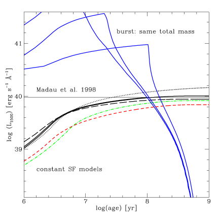
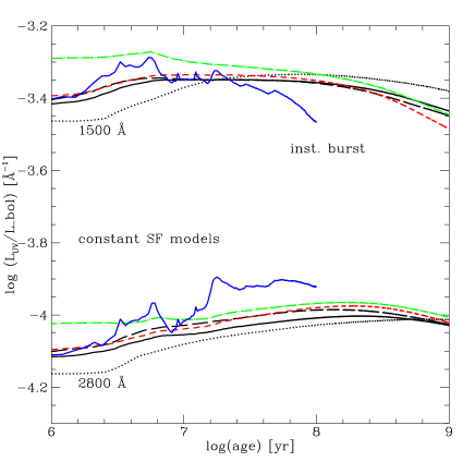
Figure 1: Left: Temporal evolution of $L_{1500}$ for models with constant SF ($SFR=1$ M_⊙ yr^-1, see Table 1 for symbols), and burst models. The SFR(UV) calibration from Madau et al. (1998, our Eq. 1) is shown by the horizontal line. Right: $L_{\rm UV}$/$L_{\rm Bol}$ for 1500 and 2800 Å for const SF and instantaneous burst models.

3 SFR from the UV continuum

The UV continuum generally probes emission from young stars so that it is a reasonable measure of ongoing star formation. The exception are elliptical galaxies and spiral bulges showing the “UV upturn” phenomenon, likely due to so-called AGB-manqué stars (e.g. Dorman et al. 1995). The optimal wavelength range is $\sim$ 1250-2500 Å, longward of the Ly$\alpha$ forest but at wavelengths short enough to minimize the contribution from older stellar populations. References to UV observations are e.g. found in the review of K98.

Many different calibrations of the SFR from the UV flux have been published (e.g. Buat et al. 1989, Deharveng et al. 1994, Meurer et al. 1995, Cowie et al. 1997, Madau et al. 1998) for $\lambda\sim$ 1500-2800 Å. According to K98 these calibrations differ by up to $\sim$ 0.3 dex when converted to a common wavelength and IMF, and differences stem from the use of various stellar libraries and different assumptions of the star formation timescales. The latter effect seems to be dominant (cf. below).

For a Salpeter IMF from 0.1 to 100 M_⊙ the calibration of Madau et al. (1998) yields

$${\rm SFR}({M_{\odot}}\,{\rm yr}^{-1})=1.4\times 10^{-28}L_{\nu}({\rm erg\,s^{-1}\,Hz^{-1}})$$ (1)

according to K98. This expression is valid for wavelengths $\sim$ 1500-2800 Å, since the resulting UV spectrum is nearly flat in $L_{\nu}$ (cf. K98). It has been obtained from the latest Bruzual & Charlot (1998) models and represents the asymptotic UV flux obtained for a exponentially decreasing SFR (cf. Madau et al. 1998).

To illustrate the dependence on metallicity, IMF, and star formation history we show in Fig. 1 (left) the temporal evolution of the UV luminosity $L_{1500}$ obtained from different models (see Table 1 for parameters and symbols used). After an initial increase the UV luminosity of the constant SF model reaches an asymptotic value at ages  $>$$\sim$ 10^8-9 yr, which is essentially identical to the one from Eq. 1 obtained for SFR $\propto\exp^{-t/\tau}$. This relatively long “equilibrium timescale” ($\tau_{\rm UV}\sim$ 1 Gyr) implies in particular that at very high redshift (typically $z~{}\hbox to0.0pt{$>$\hss}{\lower 4.30554pt\hbox{$\sim$}}$4) this situation may not be reached yet. For younger bursts producing less UV light for a given star formation rate, the SFR derived from $L_{\rm UV}$ would be higher than given by Eq. 1. The calculations for metallicities between 1/20 and 2 Z_⊙ show typically differences of 0.2 dex. Decreasing the upper mass cut-off to 30 M_⊙ or using a steeper IMF slope changes the $L_{\rm UV}$–SFR relation by a similar amount. We identify the spread between all constant SF models at equilibrium ($\sim$ 1 Gyr) as a “typical uncertainty” due to the metallicity dependence, and the slope and $M_{\rm up}$ of the IMF. For SFR($L_{\rm UV}$) this is found to be $\sim$ 0.4 dex.

In Fig. 1 (left) we also show three burst models with a duration of 5, 20, and 100 Myr forming the same mass of stars (i.e. $10^{9}$ M_⊙) as the constant SF models over 1 Gyr. Obviously such scenarios show a very different temporal evolution of the UV light, and no simple $L_{\rm UV}$-SFR relation holds. However, if the observations include a sufficiently large number of such SF regions sampling all ages, Eq. 1 yields again the correct total SFR.

The right panel in Fig. 1 shows the ratio of $L_{\rm UV}$/$L_{\rm Bol}$ for instantaneous (delta) bursts and constant SF. A fairly tight relation is expected between these quantities, quite independently of the SF history. This property may be used for SFR cross calibrations between the IR and UV (see Sect. 4).

As mentioned earlier, extinction is a major issue regarding the determination of SFRs from the UV. Although justice cannot be given to this subject here, it is, however, useful to recall a particular feature of the UV spectrum which enables such corrections in an efficient way. Indeed, a fairly narrow range of values of the UV slope $\beta$ is expected, at least for constant SF (e.g. Meurer et al. 1995, 1997). Together with the finding of empirical correlations between $\beta$ and the extinction from the Balmer decrement (Calzetti et al. 1994, 1996) and $\log(F_{\rm FIR}/F_{2200})$ which shows that dust absorption correlates with UV reddening (Meurer et al. 1995, 1997), this can be used to correct, at least in a statistical sense, for extinction. This method has been successfully applied to starburst galaxies by Meurer et al. (1997, 1999). Other methods have e.g. been used by Buat and coworkers (e.g. Buat 1992, Buat & Xu 1996, Buat & Burgarella 1998). Additional information and a summary of studies related to star formation rates using UV methods is found in K98.

Summary: From the above we conclude that the most important assumptions entering the calibration of SFR from the UV continuum are: the SF history, the IMF slope and $M_{\rm up}$, the latter two being approximately of the same importance. The “typical uncertainty” (as “defined” by the test calculations shown above) due to metallicity, IMF slope, and $M_{\rm up}$  is $\sim$ 0.4 dex. Extinction corrections, treated as “external” in this context, are obviously of prime importance for this SFR indicator.

4 SFR from the far-IR and radio continuum

4.1 Far-IR methods

At the basis for the use of the far-IR (FIR) continuum as a measure of star formation are the facts that 1) a significant fraction of the bolometric luminosity of a galaxy is absorbed by interstellar dust and re-emitted in the thermal IR, and 2) the absorption cross section of dust strongly peaks in the UV which traces young stellar populations.

The most simple assumption used for calibrations with synthesis models is that the FIR luminosity (as e.g. measured from 8-1000 $\mu$m) represents the total bolometric luminosity, or in other words that the dust is optically thick in the SF regions. This may e.g. be the case in IR luminous galaxies. In general the physical situation is, however, more complex. Different dust components (warm dust, cirrus) can be found, old stars and AGN may contribute to the heating of dust, and the optical thickness (or equivalently the reprocessing or transfer efficiency) may vary (see e.g. references in K98). No accurate universal SFR(IR) indicator can thus be expected.

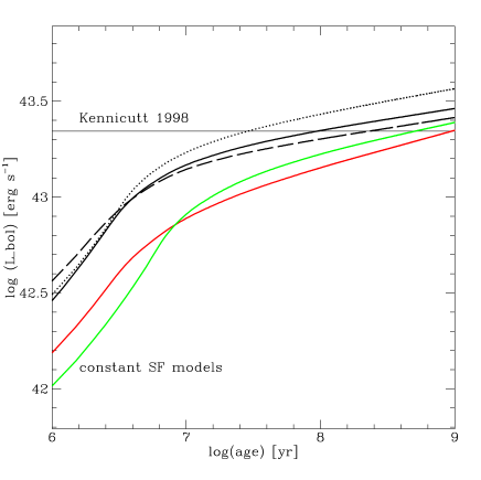
Figure 2: Same as Fig. 1 (left) for models with $SFR=1$ M_⊙ yr^-1. The Kennicutt (1998a) relation is shown by the horizontal line.

Various calibrations based on synthesis models have been published (e.g. Hunter et al. 1986, Meurer et al. 1997, Kennicutt 1998b). With the assumption $L_{\rm FIR}$=$L_{\rm Bol}$ and using the same IMF as in Eq. 1

$${\rm SFR}({M_{\odot}}\,{\rm yr}^{-1})=4.5\times 10^{-44}L_{\rm FIR}({\rm erg\,s^{-1}})$$ (2)

is obtained by K98 from the mean $L_{\rm Bol}$ for 10-100 Myr continous bursts at solar metallicity according to the Leitherer & Heckman (1995) models. Although according to K98 most other published calibrations lie within $\pm$ 30 % of this equation, e.g. the frequently used value of Thronson & Telesco (1986) is a factor of 3.8 larger for the same IMF. Most important, and larger than this, is in any case the uncertainty due to the adoption of an appropriate age for the stellar population. This is also illustrated in Fig. 2 which shows the temporal evolution of $L_{\rm Bol}$ for different models of constant SF. For obvious reasons the bolometric luminosity evolves on longer timescales than e.g. $L_{\rm UV}$, and an “equilibrium value” is not reached before $~{}\hbox to0.0pt{$>$\hss}{\lower 4.30554pt\hbox{$\sim$}}10^{10}$ yr. An assumption on the typical age or an appropriate mean age has thus to be adopted. As estimated from the model calculations illustrated in Fig. 2 the typical uncertainty due to the metallicity, IMF slope, and $M_{\rm up}$ is $\sim$ 0.3 dex.

Whereas Eq. 2 should be quite appropriate for starbursts with ages  $<$$\sim$ 10⁸ yr, the relation will be more complicated in normal star forming galaxies: a contribution from old stars to dust heating will lower the coefficient in Eq. 2, whereas the lower dust optical depth will increase this value. In this case one may refer to indirect calibrations (“cross calibrations”). E.g. for galaxies of Sb types and later one obtains ${\rm SFR}=1.1^{+1.2}_{-0.4}\times 10^{-43}L_{\rm FIR}$ (same units as Eq. 2) from the work of Buat & Xu (1996) based on a comparison of IRAS and UV flux measurement and appropriate extinction corrections, after a consistent UV calibration (Eq. 1) is applied. In a similar vein Roussel et al. (these proceedings) provide a SFR calibration for measurements using IR filters aboard ISO based on a cross calibration with an $\rm H{\alpha}$ calibration. Their spatial analysis in particular also allows one to distinguish contributions from old stars and/or AGN in the central regions.

Summary: The most important assumptions entering SFR(IR) calibrations are: the SF history or “mean age” of the population and a large dust optical depth. The “typical uncertainty” due to metallicity, IMF slope and $M_{\rm up}$  is $\sim$ 0.3 dex. One of the main advantages of this method is obviously the negligible effect of dust extinction.

4.2 SFR from radio measurements

The existence of a tight correlation between the radio (1.49 GHz) and FIR luminosity for normal galaxies has in particular motivated studies of the star formation rate from radio observations (see the review of Condon 1992). Possible AGN contamination must be accounted for. Based on the observed relationship between the radio luminosity and the supernova rate (cf. Condon & Yin 1990), Condon (1992) has derived a SFR-$L_{\rm radio}$ calibration. See e.g. Cram et al. (1998) for a recent discussion of uncertainties related to this calibration. Synthesis models including radio emission are e.g. Mas-Hesse & Kunth (1981) and Lisenfeld et al. (1996).

The above studies include in general non-thermal and thermal radio emission, the former dominating in most cases (cf. Condon 1992). From a measurement of the thermal component (if possible) the ionizing photon flux can be derived in a fairly straightforward way. Its relation to the SFR is discussed in Sect. 5.

Cram et al. (1998) present an interesting comparison of SFR indicators from FIR, radio, $\rm H{\alpha}$, and the U-band based on fairly large sample of objects. Recent examples of applications of observations to studies of the star formation history of objects up to $z~{}\hbox to0.0pt{$<$\hss}{\lower 4.30554pt\hbox{$\sim$}}1$ are e.g. found in Serjeant et al. (1998) and Mobasher et al. (1999).

5 SFR from recombination lines

Nebular lines re-emit effectively the radiation emitted shortward of the Lyman limit, and are hence a direct probe of the massive star population. In particular the hydrogen recombination lines measure directly the total ionizing photon flux. E.g. for Case B recombination the $\rm H{\alpha}$ luminosity is given by $L($$\rm H{\alpha}$)$=1.3610^{-12}f_{\gamma}\,Q_{0}$, where $f_{\gamma}$ is the fraction of photons absorbed by gas and $Q_{0}$ the total number of Lyman continuum photons ([$s^{-1}$]). This expression depends only weakly on electron temperature and density ($T_{e}=$10000 K assumed here). Corresponding expressions for other H recombination lines are readily derived.

Again, numerous calibrations based on synthesis models are found; e.g.  Kennicutt (1983, 1998ab) Gallagher et al. (1984), Leitherer & Heckman (1995), Gallego et al. (1996), Madau et al. (1998). According to K98 the calibrations are typically within  $<$$\sim$ 30 % when placed on the same IMF scale and assuming SF equilibrium (see below). Differences reflect usually changes in stellar and atmosphere models. An exception is the calibration by Alonso-Herrero et al. (1996), used e.g. in the study of Guzman et al. (1998), which yields SFRs lower by a factor 2.5. The difference appears to be due to difficulties with the former version of the Bruzual & Charlot (1993) models used by these authors (Alonso-Herrero 1999, private communication); although its origin is not yet clear, this difference is not present in their latest model version (cf. Madau et al. 1998).

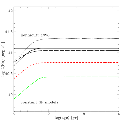
Figure 3: Left: same as Fig. 2 for $\rm H{\alpha}$. Right: Variation of the SFR($\rm H{\alpha}$) calibration (in arbitrary units) with the upper mass cut-off for a Salpeter and Scalo (1986) IMF.

Again using the same IMF as earlier, K98 obtains the following calibration:

$${\rm SFR}({M_{\odot}}\,{\rm yr}^{-1})=\frac{7.9\times 10^{-42}}{f_{\gamma}}\frac{{L_{\rm H\alpha}}}{\rm erg\,s^{-1}}\,A({\rm H{\alpha}})=\frac{1.08\times 10^{-54}}{f_{\gamma}}\,Q_{0}\,A(H\alpha)$$ (3)

where $A({\rm H{\alpha}})$ stands for the extinction at $\rm H{\alpha}$. This value is derived from a constant SF model at “equilibrium”, which is reached on a very short timescale ( $<$$\sim$ 10 Myr, see Fig. 3) due to the short lifetime of massive stars ( $>$$\sim$ 20 M_⊙) responsible for the ionizing flux. This relation may also be valid for an ensemble of burst populations of finite duration, provided enough populations of all ages up to $t_{\rm eq}$ are sampled. As shown in Fig. 3 variations by typically a factor 2 are obtained for metallicities $Z$ between 1/20 and 2 Z_⊙. E.g. at lower $Z$ a given population produces more ionizing flux, i.e. the SFR should be corrected downwards. Note that this difference is predominantly due to changes in the evolutionary tracks which are predicted to be hotter on average; changes in atmosphere models are of minor importance (e.g. Mas-Hesse & Kunth 1991).

Due to the strong increase of the ionizing luminosity with stellar mass which largely overwhelms the lifetime decrease, SFR indicators based on a measure of the Lyman continuum flux depend strongly on $M_{\rm up}$ and the slope of the upper end of the IMF. This fact which is rarely appreciated, is illustrated in both panels of Fig. 3 (see also Leitherer 1990). In particular the right panel shows the sensitivity of the $\rm H{\alpha}$ indicator on $M_{\rm up}$ for a Salpeter and Scalo (1986) IMF. E.g. a decrease e.g. $M_{\rm up}$ from 100 to 60 M_⊙ implies an increase of the SFR by a factor of $\sim$ 2 for a Salpeter IMF.

Extinction taken apart, other potential difficulties affecting the SFR($\rm H{\alpha}$) indicator are the possible escape of ionizing photons from the observed region/galaxy and the existence of dust inside the Hii regions. From studies of individual Hii regions and diffuse ionized gas in nearby galaxies (e.g. Oey & Kennicutt 1997, Ferguson et al. 1996, and references in K98) escape fractions of up to $\sim$ 15–50 % are found. Regarding the escape from the entire galaxy this value is probably lower (e.g. Leitherer et al. 1995, Deharveng et al. 1997). The quantity of dust inside Hii regions competing for the absorption of ionizing photons is not well known. Often quoted value are $\sim$ 25 % from Smith et al. (1975). New results from ISO observations should hopefully become available in the near future.

Summary: The most important assumptions entering SFR($\rm H{\alpha}$) calibrations are: the upper mass cut-off and the slope of the upper end of the IMF. This method has the shortest equilibrium timescale ( $<$$\sim$ 10 Myr) and is therefore independent on the SF history except for very “local” applications. The “typical uncertainty” due to metallicity, IMF slope, and $M_{\rm up}$  is $\sim$ 0.7 dex.

6 SFR from forbidden lines

In contrast to recombination lines, the emission of forbidden and fine-structure lines is not directly coupled to the ionizing luminosity, but depends on the ionization parameter (reflecting a combination of the ionizing luminosity, gas density, filling factor, and geometry) and the chemical composition of the gas. Therefore one usually resorts to empirical calibrations. The strong [O ii] $\lambda$3727 forbidden-line doublet discussed next is frequently used, in particular since it is accessible to optical observations over a wide range of redshifts. The potential use of other lines, including IR fine-structure lines, and results from theoretical calibrations are presented in Sect. 7.

6.1 [O ii]

Three empirical “cross” calibrations of the [O ii] $\lambda$3727 indicator through $\rm H{\alpha}$ are found in the literature. Gallagher et al. (1989) find the empirical relation $f(OII)=3.2f(H\beta)$ from a sample of irregular galaxies. For a sample of normal and peculiar galaxies Kennicutt (1992) obtains: [O ii]/([N ii]+$\rm H{\alpha}$)=0.31 and [N ii]/$\rm H{\alpha}$=0.5. From the Terlevich et al. (1991) sample of Hii galaxies Guzmán et al. (1997) find: $\langle{L_{\rm H\alpha}}A({\rm H{\alpha}})/{L_{\rm OII}}\rangle=7.42\pm 1.23$. The first two relations represent the mean values uncorrected for extinction; the last expression includes individual extinction corrections. Adopting for consistency a common $\rm H{\alpha}$ calibration (Eq. 3 with $f_{\gamma}=1$) one obtains:

$${\rm SFR}({M_{\odot}}\,{\rm yr}^{-1}) = 8.9\times 10^{-42}\,\frac{L(OII)}{{\rm erg\,s^{-1}}}\,A(H\alpha)$$ (4)

$$= 1.7\times 10^{-41}\,\frac{L(OII)}{{\rm erg\,s^{-1}}}\,A(H\alpha)=4.7\times 10^{-41}\,\frac{L(OII)}{{\rm erg\,s^{-1}}}$$ (5)

$$= 5.9\times 10^{-41}\,\frac{L(OII)}{{\rm erg\,s^{-1}}}$$ (6)

for the Gallagher et al., Kennicutt (1992) and Terlevich et al. samples respectively. K98 suggests the use of an average of Eqs. 4 and 5 with a coefficient $c=1.4\pm 0.4\times 10^{-41}$. As an example Eq. 5 is also given applying the average extinction correction of 1.1 mag derived for nearby spirals (Kennicutt 1983, 1992). Note, however, that such a correction is only consistent if derived from the entire sample used to establish the empirical [O ii]-$\rm H{\alpha}$ relation.

What is the origin of the differences between the above calibrations ? The higher SFR obtained for the Terlevich et al. (1991) sample could be due to a breakdown of the SF equilibrium assumption entering Eq. 3. Indeed it is well known that these objects are mostly of bursting nature as opposed to long lasting star formation (e.g. Stasińska & Leitherer 1996). This fact and a bias for preferentially young objects could explain why a larger SFR is obtained. Other possible explanations are mentioned below.

Some of the uncertainties of the [O ii] SFR indicator are discussed in K98. First the calibrated properties ([O ii] $\lambda$3727/$\rm H{\alpha}$, [N ii]/$\rm H{\alpha}$) show a considerable scatter in the samples used. Second, [O ii] may be enhanced by contribution from the diffuse ionized gas in starburst galaxies. More generally, however, one must make sure that the samples used for the above calibration are indeed representative for the considered application. From a comparison of $L_{\rm UV}$ and $L_{\rm OII}$, Cowie et al. (1997) find a reasonable agreement with the Gallagher et al. calibration including a modest extinction correction. Indirect evidence that the Kennicutt (1992) relation (Eq. 5) including $A({\rm H{\alpha}})=$ 1.1 mag may not apply to the CFRS sample (redshifts 0 $\leq z\leq$ 1.3) has been found by Hammer et al. (1997), although the excess of the present stellar mass density found by these authors could also simply be due to the neglect of the flattening of the IMF at low masses (see Sect. 2). Clear evidence for considerable variations of the relation between [O ii] and $\rm H{\alpha}$ emission is found by Jansen (these proceedings) in their “Nearby Field Galaxy Survey” (Jansen et al. 1999). The properties of galaxies from the Stromlo-APM survey are discussed by Loveday (these proceedings) and Tresse et al. (1999).

As K98 we conclude that [O ii] $\lambda$3727 provides a very useful estimate of the SFR in distant galaxies, and is especially useful for a consistency check on other SFR indicators. With the help of more complete samples, systematics of the [O ii] indicator will be better understood and the accuracy of calibrations improved. New calibrations, based e.g. on correlations with $L_{\rm UV}$ (e.g. Cowie et al. 1997, Hammer & Flores 1997, Fig. 1) might also be used. Alternatively, new insight can be gained from theoretical modeling. Such an approach is presented below.

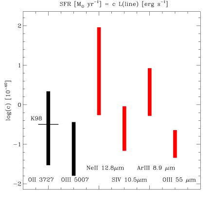
Figure 4: Left: Emission line ratio diagram for representative models with $Z=$0.004 (circles, squares, triangles) and 0.02 (solar; plus, asterisk, cross, star) and increasing ionization parameter. The solid line indicates the sequence of Baldwin et al. (1981). Right: Range of $\log c$ (in units of $10^{-40}$, for a 0.1-100 M_⊙ Salpeter IMF) predicted for various forbidden optical and IR fine-structure lines from models in the left panel. The empirical [O ii] calibration (excluding extinction) of K98 is also indicated.

7 A new approach to forbidden and fine-structure lines

To study the behaviour of [O ii] $\lambda$3727 and other potential SFR indicators from optical and IR lines we have calculated extensive grids of photoionization models for starbursts covering different SF scenarios, various metallicities, and variations of the ionization parameter, gas density, and nebular geometry. Ionizing fluxes are calculated using the synthesis models of Schaerer & Vacca (1998). We here present preliminary results (see Schaerer & Stasińska, in preparation; cf. Charlot 1998 for a similar approach).

Fig. 4 (left) illustrates an emission line diagram for representative models with constant SF, metallicities $Z=$0.004 and 0.02 (solar), and varying ionization parameter. As expected theoretically, no simple dependence of $L_{\rm OII}$ on SFR is found. For $SFR=c\,{L_{\rm OII}}$, $c$ is primarily a strong function of metallicity and the ionization. For a given metallicity $c$ increases towards models of higher excitation, reflecting the decreasing fraction of nebular luminosity emitted by the [O ii] $\lambda$3727 line. Over the parameter space explored by the models of Fig. 4 the “calibration constant” $c$ varies by a factor of up to 70 (cf. right panel)! This covers probably a parameter space larger than that populated by “real objects”. For a more realistic estimate of the uncertainty of SFR([O ii]) or theoretical calibrations various observational constraints must be taken into account.

Many other nebular lines could in principle serve as SFR indicators (cf. Sodré & Stasińska 1999). In particular the use of IR fine structure lines probing the youngest stellar populations could be of interest for objects where the IR hydrogen recombination lines cannot be measured or as an alternative or complement to IR continuum methods, whose calibration depends strongly on the SF history (Sect. 4). As for [O ii] $\lambda$3727, the expected range for $c$ for some of the strongest metal lines in the optical and IR ([O iii] $\lambda$5007, [Ar iii] 8.9 $\mu$m, [Ne ii] 12.8 $\mu$m, [S iv] 10.5 $\mu$m, [O iii] 52 $\mu$m) are shown in Fig. 4 (right). Work is underway to understand the behaviour of these potential indicators. In addition to the complexity of the parameter space of these models which must be taken into account for such “calibrations”, the IR lines are in particular affected by uncertainties related to atomic data of Ne, Ar, and S (cf. Oliva et al. 1996, Schaerer & Stasińska 1999). More detailed work on the modeling of IR lines is urgently needed to allow reliable quantitative studies of the massive star content from IR spectra (cf. Lutz et al. 1998, Schaerer & Stasińska 1998).

8 Summary and conclusions

We have reviewed the major SFR indicators (UV, FIR, $\rm H{\alpha}$, [O ii] $\lambda$3727) as well as the methods, assumptions, and uncertainties underlying these tools. All indicators rely on a calibration with evolutionary synthesis models, which depend in turn on assumptions on the IMF, the SF history, metallicity $Z$, stellar tracks and atmospheres. Extinction, which in particular strongly affects UV studies, is not discussed here. To quantify a “typical uncertainty” related to assumptions on $Z$, the IMF slope and $M_{\rm up}$ test calculations have been presented (parameters given in Table 1). Uncertainties defined in this way are $\sim$ 0.3 dex or larger for all cases.

The FIR method show the strongest dependence on the assumed SF history. Measurements related to UV light do so to a lesser degree, since the associated timescales are shorter ($\sim 10^{8-9}$ yr). The $\rm H{\alpha}$ indicator (and in principle also [O ii]) measuring the ionizing continuum produced by massive stars provide the best measure of instantaneous ( $<$$\sim$ 10 Myr) SF. However, the tradeoff of these methods is a much stronger dependence on the upper end of the IMF (slope, $M_{\rm up}$), which per se is only a bad tracer of the total mass, mostly locked up in low mass stars.

Empirical “cross” calibrations of SFR indicators from the IR, radio, and the forbidden [O ii] $\lambda$3727 lines have also been summarised. For the latter we have in particular discussed the dependence on the calibration sample. Using theoretical starburst and photoionization models we have illustrated expected variations in calibrations of forbidden lines and pointed out the interest of IR fine-structure lines for SFR determinations.

The accuracy of SFR determinations can obviously be improved by the use of multi-wavelength observations which allow to constrain and test at least some of the assumptions made in the calibrations. Sound comparisons should consider different SF indicators for the same object. Work in this direction has begun (e.g. Meurer et al. 1995, Cram et al. 1998, Pettini et al. 1998, Glazebrook et al. 1999, and references in Sect. 6). Although relative comparisons of the SFR in different environments, at different redshifts etc. can reasonably be made at present times, the slope and cut-off of the IMF at low masses remains the major uncertainty in determinations of absolute star formation rates. Both theoretical and observational progress should allow to improve our knowledge on the IMF and possible variations of it, and to study the process of star formation from the distant to the local universe.

Acknowledgments Jonathan Braine, Claus Leitherer, Gerhard Meurer and Grazyna Stasinska provided useful comments on an earlier version of the manuscript.

References

- [1] Alonso-Herrero, A., et al., 1996, MNRAS 278, 417
- [2] Baldwin, J., Philips, M., Terlevich, R., 1981, PASP 93, 5
- [3] Bruzual, G., Charlot, S., 1993, Astrophys. J. 405, 38
- [4] Bruzual, G., Charlot, S., 1998, in preparation
- [5] Buat, V., 1992, Astr. Astrophys. 264, 444
- [6] Buat, V., Burgarella, D., 1998, Astr. Astrophys. 334, 772
- [7] Buat, V., Deharveng, J.M., Donas, J., 1989, Astr. Astrophys. 223, 42
- [8] Buat, V., Xu, C., 1996, Astr. Astrophys. 306, 61
- [9] Calzetti, D., Kinney, A.L., Storchi-Bergmann, T., 1994, Astrophys. J. 429, 582
- [10] Calzetti, D., Kinney, A.L., Storchi-Bergmann, T., 1996, Astrophys. J. 458, 132
- [11] Charlot, S., 1998, in NGST - Science Drivers & Technonogical Challenges, 34th Liege Astrophysics Colloquium, eds. Benvenuti, P. et al., ESA-SP 429, p. 135
- [12] Condon, J.J., 1992, ARA&A 30, 575
- [13] Cram, L., et al., 1998, Astrophys. J. 507, 155
- [14] Cowie, L.L, et al., 1997, Astrophys. J. 481, L9
- [15] Deharveng, J.M., et al., 1994, Astr. Astrophys. 289, 715
- [16] Deharveng, J.M., et al., 1997, Astr. Astrophys. 325, 1259
- [17] Dorman, B., O’Connell, R.W., Rood, R.T., 1995, Astrophys. J. 442, 105
- [18] Ferguson, A.M.N., et al., 1996, Astron. J. 111, 2265
- [19] Gallagher, J.S., Bushouse, H., Hunter, D.A., 1989, Astron. J. 97, 700
- [20] Gallagher, J.S., Hunter, D.A., Tutukov, A.V., 1984, Astrophys. J. 284, 544
- [21] Gallego, J., et al., 1995, Astrophys. J. 455, L1
- [22] Gilmore, G., Parry, I., Ryan, S., (Eds.), 1998, ASP Conf. Series 142
- [23] Glazebrook, K., et al., 1999,MNRAS in press, (astro-ph/9808276)
- [24] Goldader, J.D., et al., 1997, Astrophys. J. 474, 104
- [25] Guzmán, R., et al., 1997, Astrophys. J. 489, 559
- [26] Hammer, F., Flores, H., 1998, in Dwarf Galaxies and Cosmology, XVIIIth Moriond astrophysics meeting, in press, (astro-ph/9806184)
- [27] Hammer, F., et al., 1997, Astrophys. J. 481, 49
- [28] Hunter, D.A., et al., 1986, Astrophys. J. 303, 171
- [29] Jansen, R.A., et al., 1999, Astrophys. J. Suppl. Ser. submitted,
- [30] Kennicutt, R.C., 1983, Astrophys. J. 272, 54
- [31] Kennicutt, R.C., 1992, Astrophys. J. 388, 310
- [32] Kennicutt, R.C., 1998a, ARA&A 36, 189 (K98)
- [33] Kennicutt, R.C., 1998b, Astrophys. J. 498, 541
- [34] Kroupa, P., 1998, ASP Conf. Series 134, 483
- [35] Kroupa, P., et al., 1993, MNRAS 262, 545
- [36] Leitherer, C., 1990, Astrophys. J. Suppl. Ser. 73, 1
- [37] Leitherer, C., Heckman, T.M., 1995, Astrophys. J. Suppl. Ser. 96, 9
- [38] Leitherer, C., et al., 1997, Astrophys. J. 454, L19
- [39] Leitherer, C., et al., 1999, Astrophys. J. Suppl. Ser. in press, (astro-ph/9902334)
- [40] Lisenfeld, U., Völk, H.J., Xu, C., 1996, Astr. Astrophys. 314, 745
- [41] Lutz, D., et al., 1998, ASP Conf. Series 132, 89
- [42] Madau, P., Pozetti, L., Dickinson, M., 1998, Astrophys. J. 498, 106
- [43] Mas-Hesse, J.M., Kunth, D., 1991, Astr. Astrophys. Suppl. Ser. 88, 399
- [44] Mateo, M.L., 1998, ARA&A 36, 435
- [45] Meurer, G., et al., 1995, Astron. J. 110, 2665
- [46] Meurer, G., et al., 1997, Astron. J. 114, 54
- [47] Meurer, G., et al., 1999, Astrophys. J. in press, (astro-ph/9903054)
- [48] Mobasher, B., et al., 1999, MNRAS in press, (astro-ph/9903293)
- [49] Oey, M.S., Kennicutt, R.C., 1997, MNRAS 291, 827
- [50] Oliva, E., Pasquali, A., Reconditi, M., 1996, Astr. Astrophys. 305, L21
- [51] Pettini, M., et al., 1998, Astrophys. J. 508, 539
- [52] Reid, I.N., Gizis, J., 1997, Astron. J. 113, 2246
- [53] Rieke, G.H., et al., 1980, Astrophys. J. 238, 24
- [54] Scalo, J., 1986, Fund. Cosm. Phys. 11, 1
- [55] Scalo, J., 1998, ASP Conf. Series 142, 201
- [56] Schaerer, D., 1998, ASP Conf. Series 131, 310
- [57] Schaerer, D., Stasińska, G., 1998, in The Universe as seen by ISO, Eds. P. Cox, M.F. Kessler, ESA Special Publications series (SP-427),in press, (astro-ph/9812068)
- [58] Schaerer, D., Stasińska, G., 1999, Astr. Astrophys. 345, L17
- [59] Schaerer, D., Vacca, W. D., 1998, Astrophys. J. 497, 618
- [60] Serjeant, S., Carlotta, C., Oliver, S., 1998, MNRAS in press, (astro-ph/9808259)
- [61] Smith, L.F., Biermann, P., Mezger, P.G., 1978, Astr. Astrophys. 66, 65
- [62] Sodré Jr., L., Stasińska, G., 1999, Astr. Astrophys. in press, (astro-ph/9903130)
- [63] Stasińska, G., Leitherer. C., 1996, Astrophys. J. Suppl. Ser. 107, 66
- [64] Terlevich, R., 1991, Astr. Astrophys. Suppl. Ser. 91, 285
- [65] Tresse, L., et al., 1999, MNRAS in press, (astro-ph/9905384)
- [66] Thronson, H.A., Telesco, C.M., 1986, Astrophys. J. 311, 98