The emission line – radio correlation for radio sources using the 7C Redshift Survey

Abstract

We have used narrow emission line data from the new 7C Redshift Survey to investigate correlations between the narrow-line luminosities and the radio properties of radio galaxies and steep-spectrum quasars. The 7C Redshift Survey is a low-frequency (151 MHz) selected sample with a flux-density limit about 25-times fainter than the 3CRR sample. By combining these samples, we can for the first time distinguish whether the correlations present are controlled by 151 MHz radio luminosity $L_{151}$ or redshift $z$. We find unequivocal evidence that the dominant effect is a strong positive correlation between narrow line luminosity $L_{\mathrm{N}LR}$ and $L_{151}$, of the form $L_{\mathrm{N}LR}\propto L_{151}^{0.79\pm 0.04}$. Correlations of $L_{\mathrm{N}LR}$ with redshift or radio properties, such as linear size or 151 MHz (rest-frame) spectral index, are either much weaker or absent. We use simple assumptions to estimate the total bulk kinetic power $Q$ of the jets in FRII radio sources, and confirm the underlying proportionality between jet power and narrow line luminosity first discussed by Rawlings & Saunders (1991). We make the assumption that the main energy input to the narrow line region is photoionisation by the quasar accretion disc, and relate $Q$ to the disc luminosity, $Q_{\mathrm{p}hot}$. We find that $0.05\raisebox{-2.58334pt}{$\,\stackrel{{\scriptstyle\raisebox{-0.60275pt}{$\textstyle<$}}}{{\sim}}\,$}Q/Q_{\mathrm{p}hot}\raisebox{-2.58334pt}{$\,\stackrel{{\scriptstyle\raisebox{-0.60275pt}{$\textstyle<$}}}{{\sim}}\,$}1$ so that the jet power is within about an order of magnitude of the accretion disc luminosity. Values of $Q/Q_{\mathrm{p}hot}\sim 1$ require the volume filling factor $\eta$ of the synchrotron-emitting material to be of order unity, and in addition require one or more of the following: (i) an important contribution to the energy budget from protons; (ii) a large reservoir of mildly-relativistic electrons; and (iii) a substantial departure from the minimum energy condition in the lobe material. The most powerful radio sources are accreting at rates close to the Eddington limit of supermassive black holes ($M_{\mathrm{B}H}\raisebox{-2.58334pt}{$\,\stackrel{{\scriptstyle\raisebox{-0.60275pt}{$\textstyle>$}}}{{\sim}}\,$}10^{9}M_{\odot}$), whilst lower power sources are accreting at sub-Eddington rates.

1 Introduction

Despite all the observational effort which has gone into researching extragalactic radio sources, we are still uncertain as to how these objects are powered and the relationship between the active nuclei, host galaxies and larger-scale environments. The current favoured models of powering extragalactic radio sources involve gas accretion onto a supermassive black hole ($M_{\mathrm{B}H}\gg 10^{6}M_{\odot}$), but details more precise than this remain controversial.

There is a strong positive correlation between the extended radio luminosities and narrow emission line luminosities of 3C radio sources (Baum & Heckman 1989; Rawlings et al. 1989; McCarthy 1993; Tadhunter et al. 1998). Rawlings & Saunders (1991, hereafter RS91) argued that by making an estimate of the bulk kinetic power in the jet from the observed low radio-frequency luminosity, it was possible to tighten this correlation (see also Falcke, Malkan & Biermann 1995). This implies that the energy source of the narrow lines is inextricably linked to the source of the radio emission. The accretion rate and/or black hole mass of the central engine are possible candidates for the connection between both types of emission. A correlation between the optical and extended-radio luminosities of steep-spectrum quasars has recently been confirmed (Serjeant et al. 1998; Willott et al. 1998a), and appears to argue strongly against alternative models in which radio and narrow-line luminosities are controlled mainly by the environment, rather than the central engine (e.g. Dunlop & Peacock 1993).

There is considerable and mounting evidence that radio galaxies and radio-loud quasars are the same objects viewed at different angles to the radio jet axis (Scheuer 1987; Barthel 1989; Antonucci 1993). A dusty torus perpendicular to the jet axis, with a high optical depth, obscures the central emission regions if the jet is roughly in the plane of the sky and a radio galaxy is observed. For objects where our line-of-sight is within the radiation cone defined by the torus, we see a luminous continuum source and broad emission lines, and the object is called a quasar. This simple model of unification by orientation appears to work remarkably well. Scattered broad emission lines have been observed in several radio galaxies (e.g. 3C 234, Antonucci 1984; 3C 324, Cimatti et al. 1996; 3C 265, Dey & Spinrad 1996; Cygnus A, Ogle et al. 1997), in accordance with the unified schemes. Near- and thermal-infrared studies (e.g. Hill, Goodrich & DePoy 1996; Simpson, Rawlings & Lacy 1999) of radio sources have revealed quasar nuclei obscured by rest-frame visual extinctions $A_{\mathrm{V}}$ in the range $0<A_{\mathrm{V}}<15$.

The narrow-line region (NLR) in radio sources is extended over several kpc, beyond the putative dusty torus, and therefore the narrow-line emission is believed to be (largely, and perhaps entirely) independent of the jet axis orientation. Similar distributions of narrow-line luminosities in samples of radio galaxies and quasars, matched in extended radio luminosity, have been suggested as a fundamental test of the unified schemes (e.g. Barthel 1989). At low redshift ($z<0.8$), there have been claims that quasars are observed to have [OIII] line luminosities a factor of 5-10 greater than radio galaxies of similar radio luminosities (Baum & Heckman 1989; Jackson & Browne 1990; Lawrence 1991). However, the [OII] luminosities of radio galaxies and quasars at low redshift are indistinguishable (Browne & Jackson 1992; Hes et al. 1993). This has been explained as partial obscuration of [OIII] emission in radio galaxies, because [OIII] is emitted from a region closer to the nucleus than [OII], due to its higher ionisation state. However, Jackson & Rawlings (1997; JR97) have investigated the [OIII] luminosities of $z>1$ radio galaxies and quasars and find their distributions indistinguishable. A possible resolution of these perceived difficulties with the unified schemes has recently been given by Simpson (1998).

Much has been learnt about radio sources from the bright 3CRR radio catalogue (Laing, Riley & Longair 1983 - LRL, see Section 2.2). However, due to the tight luminosity–redshift correlation present in a single flux-limited sample, it is impossible to distinguish whether the differences observed between 3CRR objects at high and low redshifts are correlations with redshift, or a consequence of the different radio luminosities of the sources. The best way to disentangle luminosity and redshift effects is to study a fainter radio sample and combine it with the 3CRR sample. To minimise selection effects the selection frequency of the faint sample should be close to or slightly lower than that of 3CRR (178 MHz). As discussed in detail by Blundell, Rawlings & Willott (1999a, hereafter BRW99), samples selected at significantly higher frequencies have significantly different features: namely, (i) preferential selection of Doppler-boosted objects whose radio axes are not randomly oriented with respect to the line-of-sight; and (ii) decreased sensitivity to orientation-independent steep-spectrum lobe emission. The latest published work on the radio–optical correlation in a large complete sample of radio sources (Tadhunter et al. 1998) has neither the benefits of going to fainter radio fluxes than 3CRR (for steep-spectrum objects), nor those of selecting at low radio frequencies. Allington-Smith, Peacock & Dunlop (1991) have made a limited study of emission line strengths in a 408 MHz-selected sample containing, at a given redshift, steep-spectrum objects which are slightly less radio-luminous than 3CRR objects.

We have measured the redshifts and emission line fluxes of $>90\%$ of the 77 radio sources in two of the three regions of sky which comprise the 7C Redshift Survey. A brief description of this new survey is given in Section 2.1. At a given redshift, 7C sources are a factor of $\sim 25$ times lower in luminosity than 3CRR sources. Hence, we can now for the first time clearly distinguish between redshift- and luminosity-dependent effects. In this paper we use the emission line luminosities of the 7C sources, in combination with 3CRR data from the literature, to investigate correlations between radio and emission-line properties of radio galaxies and quasars. The convention for radio spectral index, $\alpha$, is that $S_{\nu}\propto\nu^{-\alpha}$, where $S_{\nu}$ is the flux density at frequency $\nu$. We assume throughout that $H_{\circ}=50~{}{\rm km~{}s^{-1}Mpc^{-1}}$, $q_{0}=0.5$. The quantitative results are slightly different if one assumes $q_{0}=0$, as discussed in the text.

2 The complete samples

2.1 7C Redshift Survey

Only brief details of the 7C Redshift Survey are given here; full details will appear elsewhere (see also Rawlings et al. 1998, Willott et al. 1998a, 1998b, BRW99, Blundell et al. 1999b). The 7C-I and 7C-II regions contain a total of 77 radio sources which have all been identified with an optical/near-IR counterpart. These samples were selected to include all sources with flux-densities $S_{151}\geq 0.5$ Jy at 151 MHz over 0.013 sr. Spectroscopic redshifts have been obtained for all but 6 of these sources (Willott et al., in prep.). For these 6 objects, which are expected to be at $z>1$ from their $K$-band magnitudes, we have undertaken near-infrared photometry and spectroscopy in order to constrain their redshifts (Rawlings et al., in prep.). For 5 of these 6 objects, their spectral energy distributions (SEDs) are well-fitted by model elliptical galaxies with redshifts in the range $1<z<2$. The other object (5C7.47) has an unusual SED, and its redshift is firmly constrained only by the lack of a Lyman-limit cutoff in its spectrum, yielding $z<4$, but for reasons discussed in Section 2.4 we take $z=1.5$. As a result of the low selection frequency of the 7C sample, only one object (5C7.230) lies above the sample flux limit only because its core flux is Doppler boosted; this object is excluded from the analysis presented in this paper. One of the 7C sources is also in the 3CRR sample (3C 200), so excluding this too, the final 7C sample comprises 75 sources.

2.2 3CRR sample

The bright radio sample used is the 3CRR sample of LRL, which has complete redshift information for all 173 sources, selected with $S_{178}\geq 10.9$ Jy. 3C 345 and 3C 454.3 are flat-spectrum quasars which are excluded on the grounds of Doppler-boosting raising their fluxes above the selection limit. 3C 231 (M82) is excluded because it is a very nearby starburst galaxy and not a radio-loud AGN. Hence our revised 3CRR sample consists of 170 sources.

2.3 Optical classification of radio-loud AGN

Historically, quasars were defined as luminous objects with unresolved ‘stellar’ IDs and strong, broad (FWHM $>2000$ km s^-1) emission lines. In contrast, radio galaxies have a resolved optical appearance and narrow (FWHM $\approx 500$ km s^-1) or absent emission lines. However, it is now apparent that this simple classification scheme is inadequate: for example, weak quasars with host galaxies visible may be classified as broad-line radio galaxies (BLRGs). As mentioned in the introduction, spectropolarimetry of some radio galaxies has revealed broad lines scattered into our line-of-sight. It is also clear that some quasars have been reddened by dust so that the quasar is significantly dimmed in the UV (e.g. 3C 22: Rawlings et al. 1995; 3C 41: Simpson et al. 1999). Therefore the simple classification that quasars have broad emission lines must be treated with caution because, even with small amounts of reddening, this becomes dependent on redshift and whether near-infrared data is available.

For these reasons we define quasars as objects with an unresolved nuclear source which itself has absolute magnitude $M_{B}<-23$ ($q_{0}=0.5$) after eliminating light from any host galaxy and/or other diffuse continuum (such as radio-aligned emission, e.g. McCarthy et al. 1987). Some objects with broad lines have nuclei fainter than this limit. These objects will be defined in this paper simply as weak quasars (WQs). The weak quasars can be split further into three groups with sufficient polarimetric/near-infrared data; dust-reddened quasars with $A_{\mathrm{V}}\approx 1-2$, traditional broad-line radio galaxies which have intrinsically weak AGN, and radio galaxies with scattered broad lines. Two 3CRR sources have been reclassified since the classifications given in Willott et al. (1998a). 3C 318 has been found to be a quasar at $z=1.574$, not a broad-line radio galaxy at $z=0.752$ (Willott, Rawlings & Jarvis 1999). 3C 343 does not have broad emission lines in the spectrum of Lawrence et al. (1996) and is clearly resolved in the HST imaging of Lehnert et al. (1999). Therefore it is classified as a radio galaxy, not a quasar.

There are 23 quasars and 2 WQs in the 7C sample. The 3CRR sample contains 40 quasars and 13 WQs. Therefore, there are a total of 78 FRII quasars/WQs in our combined sample. There are 50 radio galaxies in the 7C sample of which only 5 have FRI structures, the rest being FRIIs or possible FRIIs (objects with a defined angular size; DAs in the notation of BRW99). To avoid confusing the issue we will hereafter refer to all objects which are not FRIs as FRIIs. In 3CRR there are 117 radio galaxies (93 FRIIs and 24 FRIs).

2.4 Narrow-line luminosities

The 245 radio sources in our combined (7C + 3CRR) sample have redshifts in the range $0<z<3$, so it is not possible to measure the flux of the same emission line in each object via optical spectroscopy. The [OII] $\lambda 3727$ line has been used for all sources where it was observed, since it is the most frequently observed narrow line in the quasars and radio galaxies in the combined sample. In cases where [OII] was not observed, other narrow lines such as [OIII] $\lambda 5007$, H$\alpha$ (RGs only), and Ly$\alpha$ (RGs only) were measured instead and converted to the expected [OII] flux using the average line ratios quoted by McCarthy (1993). Note that this method is imperfect because there exists significant scatter in the line ratios measured for radio galaxies, and evidence for some systematic changes in excitation-sensitive line ratios (like [OII]/[OIII]) with radio luminosity (Saunders et al. 1989; Tadhunter et al. 1998); it is also possible that the McCarthy line ratios are biased towards exceptionally radio luminous objects over some spectral, and hence redshift, ranges. Line fluxes and redshifts for 7C quasars and weak quasars are in Willott et al. (1998a). The spectra and line measurements of the 7C radio galaxies will be presented elsewhere (Willott et al., in prep.). The line luminosities for 3CRR sources were taken primarily from the compendia of JR97 and Hirst, Jackson & Rawlings (1999), with additional data from R. Laing (priv. comm.) and J. Wall (priv. comm.). The complete updated list of 3CRR line luminosities and their references are available on the worldwide-web at http://www.iac.es/galeria/cjw/3crr.html.

Figure 1: [OII] emission line luminosity, $L_{\mathrm{[}OII]}$, against (rest-frame) 151 MHz radio luminosity $L_{151}$ for the 7C (triangles) and 3CRR (circles) complete samples. The radio flux densities and spectral indices needed to calculate $L_{151}$ are tabulated in Blundell et al. (1999b). The sources from each sample are classified into four groups: quasars (solid symbols), weak quasars (open with a cross), FRII radio galaxies (open) and FRI radio galaxies (open with a dot). The solid lines show the power-law fits to (from top at left) (i) all the quasars and weak quasars, (ii) all sources classified as FRII, (iii) all sources classified as FRII radio galaxies.

FRI radio sources are known to have a different radio-optical correlation from FRIIs (Zirbel & Baum 1995). Of the 24 FRI radio galaxies in 3CRR, there are no emission line data in the literature for 11 of them. Therefore, we can only calculate line luminosities for about half of the 28 FRI galaxies in the combined sample. This is probably a biased subset of the true FRI population because objects with brighter lines are more likely to have had line fluxes published. Due to this incompleteness, we do not attempt to use the observed sources to investigate the FRI radio–optical correlation.

For quasars at redshifts $z\raisebox{-2.58334pt}{$\,\stackrel{{\scriptstyle\raisebox{-0.60275pt}{$\textstyle>$}}}{{\sim}}\,$}1.3$, the [OII] line passes out of the wavelength region of our optical spectra. There are few other prominent narrow quasar emission lines below the wavelength of [OII], so for most of the high-$z$ quasars, the only narrow line fluxes measured are those from the near-infrared spectrophotometry of JR97, Hirst et al. (1999) and Willott et al. (in prep.). For other high-redshift quasars the [OII] flux was estimated by calculating the continuum level at the wavelength of [OII] from the magnitudes in Willott et al. (1998a) and LRL (for 7C and 3CRR, respectively) and assuming that the rest-frame equivalent width of the [OII] line is 10Å , a typical value for ‘naked’ quasars (Miller et al. 1992). A total of 12 out of the 78 quasars in the combined sample have [OII] fluxes estimated in this way. They have a similar distribution of $L_{\mathrm{[}OII]}$ to the quasars with measured narrow lines. Use of this method, which again introduces some scatter because of the finite spread in [OII] equivalent widths for quasars, means we can include all the quasars and weak quasars in our analysis.

There are no line fluxes (or limits) in the literature for 5 of the 3CRR FRII radio galaxies. This is such a small fraction of the total number of sources that their exclusion should not significantly affect our results.

For 8 FRII radio galaxies in 7C and 2 FRIIs in 3CRR, only upper limits to the emission line luminosities are known. Where there is only an upper limit available for a line luminosity, we assume that the line luminosity is equal to this limit. One quasar from each sample has a line limit fainter than that calculated assuming an equivalent width of 10 Å, so the limit is adopted in these cases as well. There are 6 FRII radio galaxies in the 7C sample which do not have spectroscopic redshifts. For the 5 objects with redshifts well-constrained by SED fitting, we can set a limit on their H$\alpha$ fluxes from our near-IR spectra. These objects have estimated redshifts which are in the range which is traditionally difficult to measure, because no strong lines (e.g. Ly$\alpha$, [OII]) appear in the observed optical spectrum. For these objects the H$\alpha$ limits from near-infrared spectroscopy lie within the spread of the $L_{\mathrm{[}OII]}-L_{151}$ correlation, so there is no reason to expect them to have significantly weaker lines than other sources, their lack of observed emission lines being a simple consequence of their redshifts. For the object 5C7.47, we assume its redshift lies in the difficult range ($1.3\leq z\leq 1.8$), and set a limit on its line strength from our optical spectrum, associating this limit with the MgII $\lambda 2798$ line.

Sample	N	Correlated	rAB	rAB,C	signif
		variables: A,B			$\sigma$
All FRIIs	211	$L_{151},L_{\mathrm{[}OII]}$	0.784	0.635	10.78
All FRIIs	211	$z,L_{\mathrm{[}OII]}$	0.679	0.405	6.18
All FRIIs	211	$L_{151},z$	0.613	0.176	2.56
Quasars & WQs	78	$L_{151},L_{\mathrm{[}OII]}$	0.651	0.579	5.68
Quasars & WQs	78	$z,L_{\mathrm{[}OII]}$	0.539	0.427	3.92
Quasars & WQs	78	$L_{151},z$	0.366	0.023	0.19
FRII RGs	133	$L_{151},L_{\mathrm{[}OII]}$	0.794	0.617	8.18
FRII RGs	133	$z,L_{\mathrm{[}OII]}$	0.699	0.376	4.49
FRII RGs	133	$L_{151},z$	0.665	0.253	2.94

Table 1: Spearman partial rank correlation analysis of the correlations present between $L_{151},L_{\mathrm{[}OII]}$ and $z$ for various subsets of the data. This method (e.g. Macklin 1982) assesses the statistical significance of correlations between the two named variables in the presence of the third. r_AB is the rank correlation coefficient of the two variables and r_AB,C the partial rank correlation coefficient. The significance of the partial rank correlation is equivalent to the deviation from a unit variance normal distribution if there is no correlation present.

Figure 2: $L_{\mathrm{[}OII]}$ versus $z$ for all the $z>0.1$ sources only. Symbols as for Fig. 1. Note the vertical separation between 3CRR (circles) and 7C (triangles) sources, which is direct evidence that $L_{\mathrm{[}OII]}$ correlates primarily with $L_{151}$.

In conclusion, we have line luminosities or limits for 211 FRII sources out of a total of 216 FRIIs in 7C and 3CRR. We do not expect to be significantly biased in any way by the exclusion of the missing few sources, or by the 5% of cases where we have only upper limits. Using statistical techniques which account for upper limits make negligible differences to the results of this paper.

Figure 3: Emission line flux against radio flux-density for sources in the combined 7C+3CRR sample. All 229 sources are shown except 3C 274 (also known as the FRI radio galaxy M87 - excluded from this plot because its radio and [OII] fluxes are much greater than any other sources in the sample). Symbols are as for Fig. 1. The solid line goes through the median emission line and radio fluxes for each of the two samples.

3 Correlation of narrow-line and radio properties

3.1 $L_{\mathrm{[}OII]}$ versus radio luminosity, $L_{151}$

In Figure 1 we plot the [OII] line luminosity against low-frequency radio luminosity for the sample of 211 FRII sources (the 18 FRIs for which we have emission line data are also plotted). The strong correlation discussed in Section 1 is clearly apparent. The line luminosities of the 3CRR and 7C sources are about the same at radio luminosities at which the samples overlap, despite their vastly different redshifts. The best-fit power-law solutions for this correlation are plotted for several subsets of the sample (calculated by minimising the sum of the squares of the residuals). The slope of the relation for all FRII sources is $0.81\pm 0.04$ ($0.85\pm 0.04$ for $q_{0}=0$), whilst that for just the quasars and weak quasars is $0.65\pm 0.07$ ($0.72\pm 0.07$ for $q_{0}=0$). We discuss this marginally significant difference between radio galaxies and quasars in another paper (Willott et al. 1999), noting here the possibility that it is at least partly an artefact of the way in which quasars and radio galaxies are discriminated (Section 2.3; see also Simpson 1998). There is considerable scatter about the best-fit correlation of Fig. 1. This scatter is approximately gaussian in terms of $\log_{10}L_{\mathrm{[}OII]}$, with a standard deviation of 0.5.

Figure 2 plots $L_{\mathrm{[}OII]}$ against redshift for the same data. There is a clear separation between the 3CRR and 7C points, with each sample showing its own $L_{\mathrm{[}OII]}-z$ correlation which Fig. 1 shows is primarily due to the $L_{\mathrm{[}OII]}-L_{151}$ correlation rather than to an inherent $L_{\mathrm{[}OII]}-z$ correlation for radio sources. The Spearman partial rank correlation method (Macklin 1982) was used to check this result, and Table 1 shows the results of this analysis. For the combined sample, the correlation between line luminosity and radio luminosity is much stronger than the correlation of either property with $z$. However, note that there are still significant correlations between $L_{\mathrm{[}OII]}$ and $z$, independent of $L_{151}$, and $L_{151}$ and $z$, independent of $L_{\mathrm{[}OII]}$. The correlation between $L_{151}$ and $z$ is a selection effect, caused by using flux-limited samples.

The emission line flux – radio flux-density relation for the 3CRR and 7C complete samples is shown in Figure 3. It is clear that the brighter radio sources also have brighter emission lines. The median [OII] flux for 3CRR FRII sources is $2.2\times 10^{-18}$ Wm^-2. The median for 7C FRII sources (which are approximately 25 times fainter in radio flux-density than 3CRR) is $2.4\times 10^{-19}$ Wm^-2. The ratio of the median [OII] flux and the median radio flux density for the two samples implies a slope of 0.63, as plotted in Fig. 3. Given the broadly similar redshift distributions of the 3CRR and 7C samples, this is incontrovertible evidence that $L_{\mathrm{[}OII]}$ is predominantly correlated with radio luminosity, not redshift.

3.2 $L_{\mathrm{[}OII]}$ versus linear size, $D$

Figure 4: Residual emission-line luminosity (after subtraction of best-fit $L_{\mathrm{[}OII]}-L_{151}$ power-law) against projected linear size. Only FRII radio sources are plotted here. Symbols are as for Fig. 1.

We next investigate whether there is any dependence of the line luminosity on the size of the radio source, independent of the correlation with low-frequency radio luminosity. In Figure 4, we have subtracted the power-law fit of $L_{\mathrm{[}OII]}-L_{151}$ for all FRII sources from their [OII] luminosities and plot the residual against projected linear size. There is a weak anti-correlation here ($r_{DL_{\mathrm{[}OII]res}}=-0.18$, with significance 99.1%). A power-law fit gives a slope of $-0.14\pm 0.05$. Possible causes of this weak correlation and the large scatter will be discussed in Section 4.3. It is interesting to note that virtually all the relatively weak lined objects [$\Delta\log_{10}(L_{\mathrm{[}OII]})<-0.5$] have $D\stackrel{{\scriptstyle>}}{{{}_{\sim}}}100$ kpc.

3.3 $L_{\mathrm{[}OII]}$ versus low-frequency radio spectral index, $\alpha_{151}$

Figure 5: Residual emission-line luminosity against rest-frame low-frequency (151 MHz) spectral index, $\alpha_{151}$. Only FRII sources are plotted. Symbols are as for Fig. 1. The two sources with negative spectral indices (5C6.291 and 3C286) are not plotted for clarity.

Figure 5 plots the residual [OII] luminosity (after subtraction of the line–radio luminosity correlation, as in Sec. 3.2) against the rest-frame 151 MHz spectral index, $\alpha_{151}$, for all FRIIs in the sample. The Spearman rank correlation co-efficient is $r_{\alpha_{151}L_{\mathrm{[}OII]res}}=-0.105$, with significance 87%. Hence we find no evidence for a correlation between spectral index and emission line luminosity, independent of radio luminosity.

4 Discussion

4.1 The physical meaning of extended radio luminosity

4.1.1 Minimum energy formalism

For most FRII radio sources only a small fraction of the total kinetic power of the jets is released as synchrotron radiation in the lobes and hotspots. A much greater fraction is stored in the lobes and/or lost to the environment via work done by the expanding radio source (Scheuer 1974). We will define the time-averaged jet power $\bar{Q}$ as the total energy transported from the central engine by both jets divided by the age of the radio source. We reserve the symbol $Q_{o}$ to refer to the instantaneous power transported by one jet, and the symbol $Q=2Q_{o}$ for the instantaneous power of both jets, noting that these quantities might vary with time. An estimate of $\bar{Q}$ can be obtained from the minimum stored energy required in the lobes to produce the observed synchrotron luminosity, the age of the radio source, and consideration of the efficiency with which $Q$ is converted into the internal energy of the observable synchrotron-emitting population.

We first review the calculation of the minimum energy density $u_{\mathrm{m}in}$ in the lobes of a radio source (see also Leahy 1991). We will introduce various factors (denoted by $f$ and $g$) to allow for systematic uncertainties, and define these so that their values lie above unity. Cylindrical symmetry is assumed so the source has a volume, $V=\pi(D/2R_{T})^{2}D/\sin\theta$, where: $D$ is the projected linear size of the source; $R_{T}$ is the axial ratio, the ratio of the total measured length to the total measured width as defined by Leahy & Williams (1984) and Leahy, Muxlow & Stephens (1989); and $\theta$ is the angle the jet-axis makes with the line of sight. In subsequent calculations we make the approximation that $R_{T}=5$, and that $\theta=60^{\circ}$, the appropriate average value for a randomly distributed sample of radio sources; source-to-source variations in $R_{T}$ and $\theta$ will produce some scatter, but negligible systematic effects. The minimum energy density is given by (e.g. Miley 1980)

$$u_{\mathrm{m}in}=3.10^{-11}~{}\times$$

$$\left[\frac{S(1+k)\nu^{\alpha}\left(\nu_{\mathrm{l}ow}^{\frac{1}{2}-\alpha}-\nu_{\mathrm{h}igh}^{\frac{1}{2}-\alpha}\right)(1+z)^{3+\alpha}}{\sigma\eta L\left(\alpha-\frac{1}{2}\right)\sin^{3/2}\phi}\right]^{4/7}{\mathrm{J}\,m^{-3}},$$ (1)

where: $S/\sigma$ is the source surface brightness in Jy arcsec^-2; $k$ is the reciprocal of the ratio of the energy in synchrotron-radiating particles (i.e. relativistic electrons and/or positrons) to the energy in other particles (e.g. hot and/or cold protons); $\nu$, the observing frequency in GHz; $\alpha$, the radio spectral index; $z$, the redshift of the source; $\phi$, the angle between the magnetic field direction and the line-of-sight, which we set to $90^{\circ}$, and introduce a factor $f_{\rm geom}$ to account for systematically-lower values; $\eta$ is the volume filling factor; $L$ is the line-of-sight depth through the source in kpc which in our assumed geometry equals $D/(R_{T}\sin 60^{\circ})$; and $\nu_{\mathrm{h}igh}$ and $\nu_{\mathrm{l}ow}$ are the upper and lower cut-off frequencies of the synchrotron spectrum. For $\alpha>0.5$ in the radio lobes, inspection of eqn. 1 shows that $u_{\mathrm{m}in}$ is fairly insensitive to the upper cut-off frequency (we take 100 GHz), but does depends critically on the lower frequency cut-off. The true value of $\nu_{\mathrm{l}ow}$ for FRII sources is unknown because observations are not possible from the Earth for $\nu\raisebox{-2.58334pt}{$\,\stackrel{{\scriptstyle\raisebox{-0.60275pt}{$\textstyle<$}}}{{\sim}}\,$}10$ MHz. To account for this uncertainty, which is ultimately due to our ignorance of the energy density of mildly relativistic particles, we adopt a cut-off at a rest-frame frequency 10 MHz, and introduce the factor $f_{\mathrm{l}owE}$ to account for systematically-lower values of $\nu_{\mathrm{l}ow}$; note that $f_{\mathrm{l}owE}$ is a strong function of the shape of the energy spectrum of relativistic electrons, and is thus likely to vary systematically with $\alpha$. We use the symbol $u_{\mathrm{b}ase}$ to denote the evaluation of equation 1 with these assumed cut-off frequencies, with $\phi=90^{\circ}$, with $k=0$, and with $\eta=1$. This means that

$$u_{\mathrm{m}in}=\left[(1+k)f_{\rm geom}f_{\rm lowE}/\eta\right]^{4/7}u_{\mathrm{b}ase}.$$ (2)

The value of $u_{\mathrm{b}ase}$ can be calculated for a given source (of known $z$) by estimating the surface brightness at the observed frequency $\nu$ from the total monochromatic flux density at that frequency divided by the solid angle subtended by the source, again assuming a projected cylindrical geometry.

The time-averaged power of both jets $\bar{Q}$ is then given by

$$\bar{Q}=g_{\mathrm{e}xp}g_{\mathrm{k}e}\left(\frac{\left[(1+k)f_{\mathrm{g}eom}f_{\mathrm{l}owE}/\eta\right]^{4/7}f_{\mathrm{m}in}u_{\mathrm{b}ase}\eta V}{t}\right)$$ (3)

where $f_{\mathrm{m}in}$ is a factor which accounts for deviations from the minimum energy condition which corresponds to the energy density of the lobe magnetic field being about 75 per cent of the energy density of the relativistic particles. In addition to internal energy density in the lobes, we have also accounted for energy delivered by the jet, but converted into other forms: $g_{\mathrm{e}xp}$ is a factor which accounts for energy lost via the expansion work done by the radio source; and $g_{\mathrm{k}e}$ accounts for the bulk and turbulent kinetic energy of the lobe plasma. As has been known since the work of Longair, Ryle & Scheuer (1973), it is safe to neglect the gravitational potential energy of the lobe material. We have also neglected radiative losses, a point we will return to in Section 4.1.3. If we define $U_{\mathrm{b}ase}$ as $u_{\mathrm{b}ase}$ times the volume of the radio source, and absorb all the unknown factors into $f$, we obtain

$$\bar{Q}=\frac{fU_{\mathrm{b}ase}}{t},$$ (4)

The most uncertain factor in equation 3 is the value of $k$. If we assume that the material in the lobes originated in the jet, that is we assume that the radio lobes push back, and therefore exclude, any ambient material, as has been argued fairly convincingly in the case of Cygnus A (Carilli, Perley & Harris 1994), determining the value of $k$ is equivalent to determining the composition of the jet. If the jet material and hence the synchrotron-emitting lobe plasma is entirely electrons and positrons then $k=0$, whereas $k$ could, in principle, be very much higher for an electron-proton plasma: the simplest theories for particle acceleration via the shock-Fermi process suggest $k\sim 10$ (Bell 1978), and higher values are plausible (see Eilek & Hughes 1991 for a review). For this reason, we consider two models: in model A we assume that the lobe material consists entirely of electrons and positrons; in model B, protons make a significant, and perhaps dominant contribution to the energy density of the lobes. Model A is favoured by the recent detection of circular polarization in the radio cores of powerful radio sources (Wardle et al. 1998), as well as by an older dynamical argument concerning the requirements necessary for light jets to inflate lobes (e.g. Williams 1991).

It is possible to make an explicit estimate of the combined effects of the factors $g_{\mathrm{e}xp}$ and $g_{\mathrm{k}e}$. If, as is normally assumed, the material that fills the lobes passed through the hotspot regions, the points where the jets terminate, then it must have expanded from regions characterised by typical hotspot pressures $p_{\mathrm{h}s}$ to typical lobe pressures $p_{\mathrm{l}obe}\approx\frac{u_{\mathrm{m}in}}{3}$. For an adiabatic expansion, the value of $(p_{\mathrm{h}s}/p_{\mathrm{l}obe})^{x}$, with $x\approx-1/4$, measures the ratio of the internal energy of a volume element in the hotspot to that in the lobe (equation 18 of BRW99). If the ratio of these pressures scales with the radio surface brightness (see equation 1) then observations of typical hotspot and lobe surface brightnesses in FRIIs, implies that of order 50 per cent of the energy is retained as lobe internal energy, the remainder being converted to kinetic energy and/or lost as work done by the expanding lobes; since the exponent $x$ is such a small fraction, this assumption is insensitive to even fairly major departures from the minimum energy condition in one or both of the hotspot/lobe regions (Leahy 1991 and Bicknell, Dopita & O’Dea 1997 reach similar conclusions using similar arguments). We thus take $g_{\mathrm{e}xp}g_{\mathrm{k}e}\sim 2$.

In the case of model A we can further argue that kinetic energy makes such a small contribution to the energy budget that the internal energy lost is converted almost entirely into work done on the ambient material, that is $g_{\mathrm{e}xp}\sim 2$ and $g_{\mathrm{k}e}\sim 1$. Radio-emitting lobe plasma is known to be undergoing an ordered backflow from the hotspot region (e.g. Miller 1985), and spatially-resolved estimates of the ages of the lobe electrons suggest backflow speeds of up to $V_{\mathrm{b}f}\sim 0.2c$ (e.g. Liu, Pooley & Riley 1992). The kinetic energy density of this bulk flow is $\frac{1}{2}\rho V_{\mathrm{b}f}^{2}\approx\frac{2}{9}u_{\mathrm{m}in}M_{\mathrm{b}f}^{2}$ (assuming a Mach number $M_{\mathrm{b}f}$, and a relativistic equation of state for the lobe material). In model A the sound speed will be $\sim c/\sqrt{3}$, so the backflow is at most transonic ($M_{\mathrm{b}f}\sim 1$), and its kinetic energy density a small, and for our purposes negligible, fraction of $u_{\mathrm{m}in}$.

Values significantly greater than unity for most of the other unknown factors(most importantly $f_{\mathrm{l}owE}$, $1+k$ and $f_{\mathrm{m}in}$) would lead to significant increases in internal energy density, and hence pressure, from the base value of $u_{\mathrm{b}ase}$. A general, if not water-tight, argument (e.g. Leahy 1991) suggests that one can put limits on their combined effect by making a quantitative comparison of lobe pressures derived from application of equation 1 with external pressures derived by independent, typically X-ray based, techniques. In radio components bounded by weak subsonic shocks one expects that these pressures should be roughly equal, so the observation (Feretti et al. 1995) that $u_{\mathrm{b}ase}/3$ can drop to $\sim 10$ per cent of the external pressure in the tails of  head-tail’ radio sources suggests that

$$[(1+k)f_{\rm geom}f_{\rm lowE}/\eta]^{4/7}f_{\mathrm{m}in}\raisebox{-2.58334pt}{$\,\stackrel{{\scriptstyle\raisebox{-0.60275pt}{$\textstyle<$}}}{{\sim}}\,$}10.$$ (5)

The limit in this equation follows from the observation that, due perhaps to the uncertainties introduced by entrainment, the minimum pressure in the relaxed radio structures of FRI radio sources are often significantly closer to external X-ray derived pressures than those in the study of Feretti et al. (e.g. Doe et al. 1995). If one adopts a similar upward correction to the internal pressures of the lobes of classical doubles, then they are typically at a much higher pressure than their undisturbed environments: this is in keeping with the expectation that the lobes are confined by an expanding sheath of shocked gas in ram-pressure balance with the external medium (Scheuer 1974), and thus in quantitative agreement with simple models for the lobes of Cygnus A (Arnaud et al. 1984).

We can speculate further on some of the constituent parts of equation 5.

• $f_{\mathrm{g}eom}$. If the magnetic field direction is randomly distributed with respect to the line of sight, $f_{\mathrm{g}eom}\sim 1.4$.

• $f_{\mathrm{l}owE}$. The circular polarization results of Wardle et al. (1998) suggest that the distribution of electron energies extends all the way down to mildly-relativistic ($\gamma\sim 1$) energies, so that the imposition of a low-frequency cut-off at 10 MHz (corresponding to $\gamma\sim 600$ for a lobe magnetic field $B\sim 1~{}\rm nT$) leads to a significant under-estimate of the energy density in relativistic electrons. The value of $f_{\mathrm{l}owE}$ depends critically on the slope $p$ of the electron energy distribution, and, recalling that $p=2\alpha+1$, on the radio spectral index: for a $p$ of about 2, $f_{\mathrm{l}owE}\propto\ln(\nu_{\mathrm{h}igh}/\nu_{\mathrm{l}ow})$, which extrapolating to the $\gamma\sim 1$ population implies $f_{\mathrm{l}owE}\sim 2$; for $p=3$, $f_{\mathrm{l}owE}\propto\nu_{\mathrm{l}ow}^{-0.5}$, so that $f_{\mathrm{l}owE}\sim 10$ becomes plausible. The former value is likely to be appropriate unless there is evidence for a steep slope in the energy distribution from the low-frequency spectral index. We will return to this point in Section 4.3.

• $f_{\mathrm{m}in}$. Harris, Carilli & Perley (1994) argue that the most likely explanation of X-ray emission from the hotspots of Cygnus A is synchrotron self-Compton (ssC) emission, which with $k=0$ (Model A) gives magnetic field strengths very close to those estimated from the minimum energy arguments. Details of the expansion process from hotspots to lobes are required to see if this equipartition of energy densities between the particles and the magnetic field is preserved in the lobe. For a randomly oriented field and a relativistic equation of state the ratio will be preserved exactly, but if the magnetic field is ordered with respect to the flow lines then the diverging flow from the hotspot, together with flux freezing, could cause the energy density of the magnetic field to drop well below that of the particles, and $f_{\mathrm{m}in}\sim 10$ becomes plausible (Alexander & Pooley 1995), although it is not clear whether such a situation is stable. If $k\gg 0$ (Model B) then the correspondence between the X-ray flux expected from the ssC process in an equipartition magnetic field, and that observed from the hotspots of Cygnus A must be coincidental, and $f_{\mathrm{m}in}$ is unconstrained.

• $\eta$. As emphasised by Leahy (1991), there are no hard constraints on the volume filling factor. Observations of filamentary structure in the lobes of Cygnus A have been used to argue for $\eta\sim 0.1$ (Perley, Dreher & Cowan 1984; but see Tribble 1993).

Putting these considerations together for model A, equation 5 can always be satisfied for $\eta\sim 1$ if the magnetic field and particle energy densities diverge as a result of the expansion from hotspot to lobe, and/or if there is a large energy reservoir (such that $f_{\mathrm{l}owE}\sim 40$) in mildly-relativistic electrons. For $\eta\sim 0.05$ both equipartition and a low value for $f_{\mathrm{l}owE}\sim 2$ are perfectly acceptable. In the former case, combination of all the relevant factors in equation 3 suggests $f\sim 20$, whereas in the latter case $f\sim 1$. These probably bracket the uncertainties in model A.

For model B, values of $k\stackrel{{\scriptstyle>}}{{{}_{\sim}}}20$ are ruled out by equation 5 (and would require a more contrived explanation for the X-rays from the hotspots of Cygnus A) so that possible combinations of $k$, $\eta$, $f_{\mathrm{l}owE}$ and $f_{\rm min}$ again lead to the conclusion that $1<f\stackrel{{\scriptstyle<}}{{{}_{\sim}}}20$. In this case the lower bound corresponds to $k\sim 1$, $\eta\sim 0.1$, $f_{\mathrm{l}owE}\sim 2$ and $f_{\rm min}\sim 1$, and the upper bound to $k\sim 20$, $\eta\sim 1$, $f_{\mathrm{l}owE}\sim 2$ and $f_{\mathrm{}}\sim 1$. Note that the range of allowed values of $f$ is the same in both models A and B: in either model large values of $f$ require well-filled lobes, and additionally in model A the lobe plasma must either be far from equipartition or dominated by low-energy electrons. Note that RS91 took $f\approx 2$ in equation 4, which on the basis of the discussion of this section, remains a reasonable estimate.

Finally, we briefly consider ways in which $\bar{Q}$ might systematically under- or over-estimate $Q$, the instantaneous jet power of the source. Assuming a time-independent $Q$, BRW99 have presented a model for the development of an FRII radio source which suggests that $p_{\rm hs}/p_{\rm lobe}$ increases with source age, and hence with $D$, so that the ratio of work done to energy stored, and hence $Q$ to $\bar{Q}$ (as calculated with a fixed $g_{exp}\sim 2$ in equation 3), also increases systematically with $D$. However, the low value of the exponent in equation 18 of BRW99 ensures that this remains a relatively modest effect: adopting the BRW99 model $\bar{Q}/Q$ might be expected to drop by at most an order of magnitude over the range of ages, and hence $D$, spanned by FRII sources in complete samples. However, there is also a plausible mechanism for increasing $\bar{Q}/Q$ systematically with age. In a simple model in which the ratio of work done to energy stored remains constant but $Q$ decreases monotonically with source age, $\bar{Q}$ would tend to over-estimate $Q$.

4.1.2 Radio source environments

Physical models for FRII radio sources predict that sources of fixed $Q$ evolve differently with time in different gaseous environments (Scheuer 1974; Falle 1991). Any quantitative study of the FRII population must attempt to account for this effect. Unfortunately, the nature of the environments of FRII radio sources cannot be straightforwardly deduced from any existing observational data. Even at very low redshifts ($z\sim 0.1$), X-ray observations currently lack both the sensitivity and resolution to map the thermal emission from the gaseous haloes of FRII radio galaxies with the exception of a few, possibly atypical, sources like Cygnus A (Reynolds & Fabian 1996). Other probes of the environmental density, including galaxy counting (e.g. Hill & Lilly 1991), weak gravitational lensing (e.g. Bower & Smail 1997), and studies of radio polarization (e.g. Garrington & Conway 1991), are inherently indirect. We will discuss these various observational constraints in detail elsewhere (Rawlings, Willott & Blundell, in prep, hereafter RWB), and here merely state, and subsequently employ, various assumptions about typical FRII environments at both low and high redshift.

Following Falle (1991) and Kaiser & Alexander (1997) we will characterise the electron number density profile $n(r_{100})$ of the radio source environment by a power-law,

$$n(r_{100})=n_{100}r_{100}^{-\beta},$$ (6)

where $r_{100}$ is the radial distance from the active nucleus, measured in units of $100~{}\rm kpc$, and $n_{\mathrm{1}00}$ is the electron number density when $r_{100}=1$. The normalisation radius of $100~{}\rm kpc$ will be denoted as $a_{\rm o}$ in subsequent calculations. This profile is a good approximation only at radii $\sim 100~{}\rm kpc$ since the true gas density profile is likely to be concave (e.g. Navarro, Frenk & White 1997); a detailed discussion, and arguments for a generic $\beta$ value of $1.5$, will be presented in RWB; here, we simply note that this profile is a good fit to the $n(r)$ functions derived for the clusters embedding the luminous radio sources Cygnus A and 3C 295 (Reynolds & Fabian 1996; Neumann 1999).

Estimation of the normalisation parameter $n_{\mathrm{1}00}$ in equation 6 is more problematic. At low redshift ($z\sim 0.1$) FRII radio galaxies are found to be associated almost exclusively with isolated elliptical galaxies and/or poor groups of galaxies, that is environments less rich than Abell clusters (e.g. Prestage & Peacock 1988, 1989). This suggests a typical value of $n_{100}\sim 400~{}\rm m^{-3}$, but to account for low-redshift environments as poor as an isolated elliptical, and as rich as 3C 295, it can seemingly lie anywhere in the range $10^{2}\raisebox{-2.58334pt}{$\,\stackrel{{\scriptstyle\raisebox{-0.60275pt}{$\textstyle<$}}}{{\sim}}\,$}n_{100}\raisebox{-2.58334pt}{$\,\stackrel{{\scriptstyle\raisebox{-0.60275pt}{$\textstyle<$}}}{{\sim}}\,$}10^{4}~{}\rm m^{-3}$.

At higher redshifts ($z\sim 0.5-0.8$) galaxy-counting experiments (Yates, Miller & Peacock 1989; Hill & Lilly 1991; Allington-Smith et al. 1993; Roche et al 1999) show that FRIIs, covering a wide range of radio luminosity, are typically associated with rich groups, environments alternatively known as poor clusters. The significant fraction of X-ray detections amongst $z\sim 1$ 3C radio sources (Crawford & Fabian 1996), X-ray emission which in some cases is clearly extended and probably thermal, suggests that this gradual increase in environmental density persists to $z\sim 1$. This trend with redshift provides the most straightforward explanation for the systematic increase in the depolarisation of the lobes of radio quasars from redshift $z\sim 0$ to $z\sim 1$ (e.g. Garrington & Conway 1991). These results suggest a value of $n_{100}\sim 3000~{}\rm m^{-3}$ as a typical normalisation value at $z\sim 1$. Taken at face value the small scatter in the depolarisation data at high redshifts implies a fairly small spread about this value of, say, $\pm 0.25$ dex, but since the published depolarisation work is largely confined to the brightest (e.g. 3C) sources, this may be in part a selection effect. The analysis of Section 4.1.3. is, however, confined to this same bright population, and so $n_{100}=3000~{}\rm m^{-3}$ should be an appropriate normalisation factor; the consequences of systematic changes in environment with redshift will be discussed in Section 4.3.

4.1.3 Ages and head advance speeds

To determine jet powers and their relationship with the ages and sizes of radio sources, we follow the dimensional analysis of Falle (1991). He showed that the quantities $Q$, $\rho_{100}a_{\mathrm{o}}^{\beta}$ (where $\rho_{100}$ is the mass density at 100 kpc equivalent to electron density $n_{100}$), and Ṁ_J (the jet mass flux) can define a characteristic length scale, $L_{\mathrm{o}}$,

$$L_{\mathrm{o}}=\left(\frac{\left(\rho_{100}a_{\mathrm{o}}^{\beta}\right)^{2}Q}{2\dot{M}_{\mathrm{J}}^{3}}\right)^{\frac{1}{2\beta-4}}.$$ (7)

For typical FRII source parameters, $L_{\mathrm{o}}\sim 10$ pc, which is small compared to the size of radio jets. At distances much greater than $L_{\mathrm{o}}$, the mass in the bow shock is dominated by material swept up by the jet, so Ṁ_J is unimportant. This leads to a bow-shock which is self-similar, the future dynamics of which can be determined by a simple dimensional analysis. Kaiser & Alexander (1997) argued that the self-similar growth also applies to the cocoon excavated by the jet. BRW99 present a model in which the cocoon does not grow self-similarly ($R_{T}$ and $g_{\mathrm{e}xp}$ are slow functions of source age). In all these models, the evolution of the projected linear size of the radio source, $D$, is given by

$$\frac{D}{\sin\theta}=2c_{1}a_{\mathrm{o}}t^{\frac{3}{5-\beta}}\left(\frac{Q}{2a_{\mathrm{o}}^{5}\rho_{100}}\right)^{\frac{1}{5-\beta}},$$ (8)

where the factors of 2 come in because the linear size is the separation between the ends of each jet of power $Q/2$. $c_{1}$ is a constant unconstrained by the dimensional analysis. Re-arranging this expression to make $t$ the subject tells us how the age of a radio source is related to $D,Q$ and its environment;

$$t=\left(\frac{D}{2\sin\theta c_{1}a_{\mathrm{o}}}\right)^{\frac{5-\beta}{3}}\left(\frac{2a_{\mathrm{o}}^{5}\rho_{100}}{Q}\right)^{1/3}.$$ (9)

To constrain the constant $c_{1}$ we now consider the instantaneous head advance speeds of FRII radio sources. Using a method based on the length asymmetry between the two lobes of radio sources, Scheuer (1995) showed that radio source advance speeds derived by synchrotron ageing methods (e.g. Alexander & Leahy 1987, Liu et al. 1992) are over-estimated due to large contributions to the derived flow speeds by backflow. The samples of objects investigated by Scheuer are of the most powerful radio sources known: they have a mean radio luminosity of $\log_{10}(L_{151}$ / WHz^-1sr${}^{-1})=28.0$ and a median projected linear size of 110 kpc. Since they are mostly quasars, we take a typical angle to the line-of-sight of 45^∘. This gives a median de-projected linear size of 160 kpc – the same as that of the whole 3CRR and 7C sample. The mean head advance speed $V_{\mathrm{h}ead}$ derived by Scheuer is $0.03c$, with a firm upper-bound of $0.15c$. We adopt the typical ‘high-redshift’ environment for an FRII discussed in Section 4.1.2.

Differentiating equation 8 with respect to time (keeping $Q$ constant), we obtain the advance speed of the radio source, $v$,

$$2v=\frac{dD}{dt}=2\sin\theta c_{1}a_{\mathrm{o}}\left(\frac{3}{5-\beta}\right)t^{\left(\frac{\beta-2}{5-\beta}\right)}\left(\frac{Q}{2a_{\mathrm{o}}^{5}\rho_{100}}\right)^{\frac{1}{5-\beta}}.$$ (10)

Note the $t$-dependence of the advance speed. This shows that the advance speed is constant throughout a source’s lifetime only in a $\beta=2$ environment. For $\beta=1.5$, we find that $v\propto t^{-1/7}$, i.e. the source decelerates, albeit slowly, as it grows. Substituting $D$ for $t$ from equation 9 gives us an expression relating $v$ and $D$ for a particular value of $Q$. We find $v\propto D^{(\beta-2/3)}$ which is $v\propto D^{-1/6}$ for $\beta=1.5$. Therefore, if we know the current hotspot advance speed (inferred from Scheuer 1995), we can determine $v$ throughout the source’s lifetime and hence calculate the age of the source. We find that for $v=0.03c$ and $v=0.15c$, the typical ages of these sources are $7.4\times 10^{6}$ and $1.5\times 10^{6}$ years, respectively. Equation 10 shows that, for a given $c_{1}$, $v$ and $D$, there is a degeneracy between $Q$ and $t$. However, this degeneracy can be broken because equation 4 contains another relationship between $Q$ and $t$.

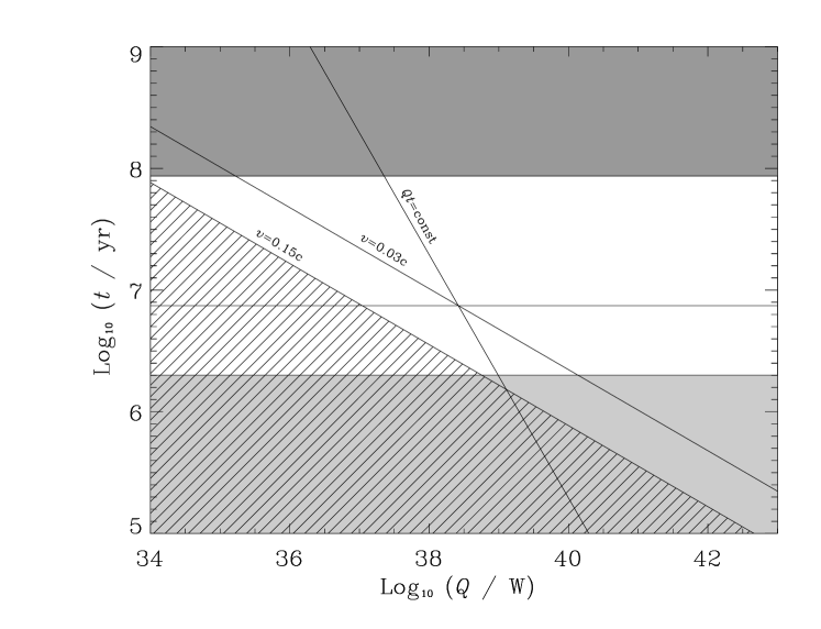
Figure 6: $Q$ versus the age of the powerful FRII sources investigated by Scheuer (1995). The line labelled $Qt$ is the energy conservation requirement of equation 4. The lines labelled $v=0.03c$ and $v=0.15c$ are from equation 10, with values of $c_{1}$ such that they intersect the $Qt$ line at the ages derived in the text. The pale shaded region shows the limit on $t$ set by the observations of Liu et al. (1992). The dark shaded region shows the limit on $t$ from the requirement that the jet be supersonic throughout its lifetime. The diagonal line shaded region is disallowed by the observations of Scheuer (1995). The intersection of the $Qt$ and $v=0.03c$ lines give our best estimate of the typical ages and jet powers of the sources used by Scheuer; $t\approx 10^{7}$ years and $Q\approx 3\times 10^{38}$ W. This diagram fixes the value of the unknown constant $c_{1}$.

Inserting the ages calculated above into equation 4 gives a unique value of $Q$ for a source of a particular age. Figure 6 plots $Q$ against $t$ from equation 4. Equation 4 is simply an energy conservation line from the minimum energy assumption. The two lines labelled $v=0.03c$ and $v=0.15c$ in Figure 6 are from equation 10, given that they intersect the line from equation 4 at the ages calculated above. They therefore each give a value of the unknown constant $c_{1}$. The region to the lower-left of the line labelled $v=0.15c$ is ruled out by the upper limit to the hotspot advance speed (Scheuer 1995).

We also have two further constraints on the regions allowed in the $Q$–$t$ plane. Spectral ages of powerful FRIIs have been determined by Liu et al. (1992). The mean age for their most powerful sources [$\log_{10}(L_{151}$ / WHz^-1sr${}^{-1})\geq 27.5$ and $D\approx 100$ kpc] is $2\times 10^{6}$ yrs. Note that this is a lower limit to their actual ages because of the arguments about the importance of backflow put forward by Scheuer (1995). An upper limit to the ages of FRII radio source comes from the requirement that the head of the radio source advances supersonically throughout its lifetime. We calculate the sound speed of the IGM assuming $T=2$ keV, an appropriate value for a rich group. Assuming that the head advance speed equals the sound speed throughout its lifetime, we derive an upper limit to the age of $10^{8}$ yrs. Note that this is a strict upper limit because we have already shown that the jet decelerates as it propagates. These upper and lower age limits are shown in Fig. 6.

The intersection of the $Qt$ and $v=0.03c$ lines give our best estimate of the typical ages and jet powers of the sources used by Scheuer. Ages of $\approx 10^{7}$ years are consistent with our strict upper and lower age limits derived above. Note that if the current hotspot advance speeds are as high as $v=0.15c$, then the calculated ages would be below the lower limit from spectral ageing. The derived jet powers are $Q\approx 3\times 10^{38}$ W. From the intersection of the $Qt$ and $v=0.03c$ lines we derive a value of the constant, $c_{1}$. This clearly depends critically on the value taken for $f$ in equation 4: for $f=1$, $c_{1}=5.4$ and for $f=20$, $c_{1}=2.3$.

Now that we have estimated $c_{1}$, it is trivial to estimate the jet power. Substituting $t$ from equation 9 into equation 4 gives

$${Q}=\left({fu_{\mathrm{m}in}V}\right)^{3/2}\left(\frac{D}{2\sin\theta c_{1}a_{\mathrm{o}}}\right)^{\frac{\beta-5}{2}}\left(2a_{\mathrm{o}}^{5}\rho_{100}\right)^{-1/2}.$$ (11)

Since $u_{\mathrm{m}in}\propto L_{151}^{4/7}$ from equation 1, we find that $Q\propto L_{151}^{6/7}$ (at fixed $D$). Hence this model predicts a relationship between the jet power and the observed extended radio luminosity which is slightly less steep than linear. $u_{\mathrm{m}in}V\propto D^{9/7}$, which gives $Q\propto D^{-4/7+\beta/2}$ (for sources with the same $L_{151}$) . Hence, for $\beta=1.5$, this gives a very weak expected $D$ dependence of $Q\propto D^{\frac{5}{28}}$. Note that very small changes in $\beta$ determine whether the derived $Q$ goes up or down with $D$ at a fixed $L_{151}$, but for realistic values of $\beta$, $Q$ is not a strong function of $D$. Therefore we find the relationship between $Q$ and $L_{151}$ in the adopted environment is given by

$$Q\simeq 3\times 10^{38}L_{151}^{6/7}~{}{\rm W},$$ (12)

where $L_{151}$ is in units of $10^{28}$ W Hz^-1 sr^-1.

We can now check one of our previous assumptions – that radiation losses are negligible compared to the time-averaged bulk kinetic power of the jet. We calculate the total energy radiated by sources with parameters similar to those investigated by Scheuer (1995). These sources have $\log_{10}(L_{151}$ / WHz^-1sr${}^{-1})\approx 28.0$ and $D=110$ kpc. The evolutionary track of a source with these parameters on the $L_{151}$-$D$ plane is approximated by a power-law, $L_{151}\propto D^{\frac{-5}{24}}$, for $\beta=1.5$ and a constant $Q$. To get a maximum value of the synchrotron energy radiated, we assume a steep spectral index ($\alpha=1$), integrate the spectrum over a (rest-frame) frequency range 10 MHz to 100 GHz, and then integrate over the source age. Note that it is possible that the synchrotron spectrum extends to lower frequencies than those observable, but that for each decade in frequency that the spectrum extends beyond this, the total energy radiated is increased only by a quarter. We find that the total synchrotron energy radiated over the sources lifetime is of the order of a few per cent of $Qt$. We are therefore clearly justified in our assumption that radiation losses make a negligible contribution to the total energy budget. This is not a surprising result because the synchrotron lifetimes of the low-energy electrons, where the bulk of the lobe particle energy is stored, are much larger than the ages over which a radio source with a typical evolutionary track keeps above the flux density limit of a complete sample (BRW99).

4.2 The physical meaning of narrow emission line luminosity

4.2.1 The excitation mechanism for the narrow emission lines

Even though the extreme ultraviolet luminosities of certain high-redshift radio galaxies are most plausibly explained by continuum emission from young hot stars, the high-excitation emission line spectra seen even in these cases demonstrate that the narrow emission lines are overwhelmingly excited by the central engine (e.g. Dey et al. 1997, and see McCarthy 1993 for a general review). There are still, however, at least four distinct physical ways in which the central engine can excite emission lines.

1. Quasar illumination. A broad (half-opening angle $\approx 50^{\circ}$) radiation cone from a central quasar ionises and heats ambient material which cools via narrow-line radiation. In the ionisation-bounded case, where individual optically-thick clouds absorb and re-radiate all the incident flux, the narrow-line luminosity is proportional to the photoionising quasar luminosity $Q_{\rm phot}$ modulo a covering factor $CF$. The small spread in the equivalent width of narrow emission lines in low-redshift quasars (e.g. Miller et al. 1992) suggest a narrow range in $CF$ and no systematic variations of $CF$ with $Q_{\rm phot}$.

2. Blazar illumination. A narrow (half-opening angle $\approx 10^{\circ}$) beam of Doppler-boosted optical/UV synchrotron emission ionises and heats material which cools via narrow-line emission. Such beams pointed towards Earth explain most of the properties of the objects known as blazars.

3. Jet-cloud collisions. Jets collide with ambient clouds transferring some fraction of their mechanical power to thermal energy via shocks driven into the clouds. Subsequent cloud cooling produces narrow line emission.

4. Bow-shock excitation. Expanding lobes of FRII radio sources do work on the ambient material mediated by a strong bow shock. If any of the material passing through this shock has sufficient time to cool to $\sim 10^{7}~{}\rm K$ then the bow shock can become radiative, so that some fraction of the power delivered to the bow-shock can emerge as bremsstrahlung and line emission. This radiation excites a proportional amount of narrow emission line luminosity provided the densest material in the bow shock has cooled to $T\sim 10^{4-5}~{}\rm K$.

We will hereafter neglect mechanisms (ii) and (iii) for exciting narrow emission lines because the bulk of the narrow emission lines in radio galaxies come typically either from nuclear regions, or from extended regions which viewed from the active nucleus cover a solid angle far larger than it is possible to achieve via mechanisms (ii) and (iii). Nevertheless, there are individual radio galaxies in which one or both of these ‘narrow-beam’ mechanisms are likely to be in operation, and which contribute significantly to the total narrow-line emission: the extranuclear emission line filaments in Centaurus A have been ascribed to both blazar illumination (Morganti et al. 1991) and jet-cloud collisions (Sutherland, Bicknell & Dopita 1993); mechanisms (ii) and (iii) have also been invoked for 3C 356 (Lacy & Rawlings 1994) and PKS2152-699 (di Serego Alighieri et al. 1989).

Deciding between mechanisms (i) and (iv) is complicated by the realisation that fast shocks produce a local photoionising source which can mimic the ionisation/heating effects of a quasar power law (e.g. Binette, Dopita & Tuohy 1985), especially when only optical line diagnostics are available (e.g. Allen, Dopita & Tsvetanov 1998). Nevertheless, there is good observational evidence that mechanism (i) is normally dominant: the major arguments are as follows.

• Accounting for differential reddening between the continuum/broad-line region and the narrow-line region, powerful steep-spectrum radio-loud quasars have the same small spread in their (rest-frame) narrow-line equivalent widths as radio-quiet quasars (Miller et al. 1992). Amongst the steep-spectrum quasars there is no evidence for any dependence of equivalent width on quasar luminosity (Jackson & Browne 1991), on redshift (at least out to $z\sim 2$; JR97), or on radio source size (Hirst et al. 1999). It thus seems hard to escape the conclusion that the quasar continuum luminosity is the principal factor which controls the narrow emission line luminosity.

• Many powerful radio galaxies show polarimetric and spectropolarimetric evidence for hidden quasar cones impinging on scattering media coincident with the narrow-line emitting gas (e.g. Tran et al. 1998 and refs. therein).

• In a study of the UV line ratios of a large sample of $z\sim 2$ radio galaxies Villar-Martin, Tadhunter & Clark (1997) concluded that the ionisation states are primarily determined by photoionisation from a central source. Detailed models of photoionising shocks (e.g. Allen et al. 1998) suggest that the UV collisionally-excited lines should be strongly boosted in the high-temperature cooling zones behind fast shocks, whereas the line ratios in $z\sim 2$ radio galaxies show no evidence of this boosting and follow closely those predicted by a quasar-illumination model.

• For objects confined to a narrow region of the $L_{151}$ versus $z$ plane, the sizeable spread in narrow line luminosity seems well correlated with the underlying quasar luminosity. The recent work of Simpson et al. (1999) illustrates this effect: they found an intrinsically ultraluminous thermal-infrared nucleus in 3C 265, a $z\sim 1$ 3C radio galaxy with ultraluminous narrow emission lines, but evidence for a weak thermal-infrared nucleus in 3C 65, the $z\sim 1$ 3C radio galaxy with the weakest narrow emission lines. The low-excitation line ratios of the weakest narrow-line emitters provides indirect evidence that they harbour intrinsically weak quasar nuclei (e.g. Tadhunter et al. 1998). Evidence of line excitation correlating positively with narrow-line luminosity was used by Saunders et al. (1989) to argue that the narrow-line luminosity is proportional to the underlying quasar luminosity in low-redshift FRII radio sources.

Evidence for the dominance of mechanism (iv) is confined to individual, possibly atypical, cases, and is largely circumstantial. It is clear, however, that shocks in general, and the bow-shock in particular, have a huge influence on the spatial structure and kinematics of the extended narrow-line emitting regions (e.g. McCarthy 1993). The key point here is that even in a pure quasar-illumination picture, the presence of shocks can have an important influence on the emergent line ratios, and some impact on the line luminosities. As the excitation level is controlled by the effective ionisation parameter $U_{e}$ (the ratio of the photon density to the electron density), and as densities are typically boosted by shock compression, the ratio of high- to low-excitation lines (e.g. [OIII] to [OII]) will, for a fixed incident photon flux, be lower in post-shock gas (Clark et al. 1997; Lacy et al. 1998). Cooling behind shocks may also introduce cool UV-opaque material at large radii which raises the $CF$ and hence the line luminosity. For these reasons, some authors (e.g. Tadhunter et al. 1998) invoke shocks to explain why some powerful narrow-line radio galaxies have ultraluminous emission lines, but relatively low excitation spectra (JR97). We note that it might be possible to obtain a more accurate indicator of the underlying quasar luminosity by restricting attention to emission line luminosity arising from the nuclear regions. We will return to this important question in Section 4.3, assuming for now that mechanism (i) is the dominant way in which the AGN delivers energy to the narrow line region.

4.2.2 The relationship between $L_{\mathrm{[}OII]}$ and $Q_{\rm phot}$

Miller et al. (1992) showed that in a complete sample of the brightest low-redshift ($z<0.5$) optically-selected quasars, the narrow emission line equivalent widths show very little scatter (0.2 dex) and are not correlated with optical luminosity. This quasar sample was taken from the Bright Quasar Survey (BQS; Schmidt & Green 1983) which because of its UV-excess selection criterion is dominated by ‘naked’ quasars in which differential reddening between the lines-of-sight to the narrow-line region and the continuum producing regions should be unimportant. Within the Miller et al. BQS sub-sample there is no evidence of any difference between the [OII] EW distributions of radio-loud and radio-quiet quasars. Differential reddening is a likely explanation for the larger means and dispersions for the distributions in [OII] equivalent widths in radio-selected samples of quasars (Jackson & Browne 1991; Baker 1997). We assume that (before any reddening) all steep-spectrum radio sources have rest-frame [OII] equivalent widths of 10 Å, which is the mean value determined by Miller et al.

Given an [OII] line luminosity and an assumed EW we can calculate the monochromatic blue luminosity. To convert this to a bolometric luminosity we use the Sanders et al. (1989) study of the spectral energy distributions of BQS quasars. Sanders et al. observe a small range in $L_{\mathrm{b}ol}/\nu L_{\nu}(B)$ in their sample, with a mean of 16.5. We take $Q_{\mathrm{p}hot}=L_{\mathrm{b}ol}$ because the big blue bump contributes at least 70% of the bolometric luminosity of quasars and at least some of the remainder (chiefly in the IR bump) may be reprocessed emission from the accreting material. With an assumed rest-frame [OII] equivalent width of 10 Å, this gives

$$Q_{\mathrm{p}hot}\simeq 5\times 10^{3}L_{\mathrm{[}OII]}~{}{\rm W}.$$ (13)

RS91 estimated $Q_{\mathrm{p}hot}$ by converting from one or two observed narrow line luminosities to $L_{\rm NLR}$ and then assumed a covering factor of $CF\sim 0.01$. Using the line ratios in McCarthy (1993) we estimate that $L_{\rm NLR}\approx 15L_{\mathrm{[}OII]}$ and the inferred covering factors ($CF\sim 0.003$) are similar to those of RS91.

4.3 The relationship between $Q$ and $Q_{\rm phot}$

In Section 4.1 we argued that the range in extended radio luminosity spanned by FRII radio sources in complete samples is controlled principally by a range in $Q$, the jet power, and gave a formula mapping $L_{151}$ to $Q$. In Section 4.2 we argued that the range in narrow emission line luminosity of FRII radio sources is controlled principally by a range in $Q_{\rm phot}$, and gave a formula mapping $L_{\rm[OII]}$ to $Q_{\rm phot}$. In this section we put these results together to investigate the origin of the emission line – radio luminosity correlation.

Figure 7: The $L_{\mathrm{[}OII]}$ versus $L_{151}$ correlation of Fig. 1, where the vertical axis now shows the photoionising power, $Q_{\mathrm{p}hot}$, instead of $L_{\mathrm{[}OII]}$. $Q_{\mathrm{p}hot}$ is calculated for each source as described in Section 4.2. The solid line is the least-squares fit to all FRIIs of Section 3. The dashed lines show the variation of $Q_{\mathrm{p}hot}$ with $L_{151}$ as calculated in Section 4 assuming $Q_{\mathrm{p}hot}=Q$. The upper dashed line is for the case of $f=20$ and the lower one for $f=1$. The dotted and dot-dashed lines show the uncertainty in the $f=1$ case due to a range of environments as discussed in the text. The right vertical axis shows the central black hole masses implied by this model for Eddington-limited accretion (which we argue in Section 4.3 is unlikely to be the case for objects with $Q_{\mathrm{p}hot}\raisebox{-2.58334pt}{$\,\stackrel{{\scriptstyle\raisebox{-0.60275pt}{$\textstyle<$}}}{{\sim}}\,$}10^{39}{\mathrm{W}}$).

We begin with the hypothesis that $Q_{\rm phot}$ is equal to the jet power $Q$. This form of behaviour is characteristic of some symbiotic jet-disc models (e.g. Falcke & Biermann 1995). Figure 7 shows the emission line–radio correlation (Fig. 1) again, with $L_{\mathrm{[}OII]}$ replaced by $Q_{\mathrm{p}hot}$ (the solid line calculated according to the prescription of Section 4.2.2). Also on this figure are lines representing the relationship between $Q$ and $L_{151}$ derived in section 4.1 (equation 12) under the assumption that $Q_{\rm phot}=Q$. The first thing to notice is that the gradients of the model lines (dashed) are very similar to the gradient of the best-fit line. The model predicts $Q\propto L_{151}^{0.86}$ and the fitted line gives $Q\propto L_{151}^{0.81\pm 0.04}$. The upper dashed line is for the case of $f=20$ (which recall from section 4.1.1 is the maximum possible energy according to the constraint of equation 5) and the lower dashed line for the absolute minimum energy case of $f=1$. We see that for $f=20$ then $Q_{\rm phot}$ and $Q$ are indeed approximately equal, whereas for $f=1$, $Q_{\rm phot}\approx 20Q$, i.e. the jets only carry 5% as much power as is released during accretion. If one instead assumes an open universe with $q_{0}=0$, then $Q_{\mathrm{p}hot}\approx 2Q$ for $f=20$ and 40$Q$ for $f=1$. Hence the ratio of jet to accretion power is half that for $q_{0}=0.5$. The slope of the best-fitting $L_{\mathrm{[}OII]}$–$L_{151}$ correlation (Section 3.1) for $q_{0}=0$ is $0.85\pm 0.04$, i.e. still consistent with the model slope of 0.86.

Dunlop & Peacock (1993) raised the possibility that the correlation between the radio luminosity, $L_{\mathrm{r}ad}$, and the narrow emission line luminosity, $L_{\mathrm{N}LR}$, is actually due to environmental effects. They noted, as we can see from equation 11, that for a given jet power, sources in higher density environments have higher radio luminosities ($L_{151}\propto\rho_{100}^{1/2}$). Given the wide variety of environments in which FRII sources are found, this is indeed likely to be a major cause of scatter in the emission line – radio correlation, but could it dominate the correlation?

To investigate environmental effects on the slope, normalisation and scatter of the correlation, we adopt the range of environments at both low- and high-redshift discussed in section 4.1.2. Recall that there is some evidence that the scatter in environments at low- to moderate-redshift (from isolated ellipticals to clusters like that associated with 3C 295) is greater than that at $z\raisebox{-2.58334pt}{$\,\stackrel{{\scriptstyle\raisebox{-0.60275pt}{$\textstyle>$}}}{{\sim}}\,$}1$. Due to the tight correlation between $L_{151}$ and $z$ in flux-limited samples, a mapping between $L_{151}$ and a typical $z$ was possible for each of the 3CRR and 7C samples. We then recalculated the $f=1$ model line assuming evolution in the upper and lower limiting density environments. Fig. 7 plots these bounds for the 3CRR (dotted) and 7C (dot-dashed) samples. It can be seen that at high luminosities the range of scatter due to environments is small, but at lower luminosities it could be responsible for about one dex of scatter. The strongest systematic effect of environment we can envisage would arise if all low power FRIIs were in isolated ellipticals and all high power FRIIs were in rich clusters. This systematic change in environment would flatten the expected $L_{\mathrm{[}OII]}-L_{151}$ correlation to a slope of $\approx 0.6$.

The emission line – radio correlation holds over four orders of magnitude, so we can rule out environmental effects as the cause of the correlation, since they can account for only a maximum difference in $L_{151}$ of one dex, corresponding to two dex in $n_{100}$ at a given $Q$. Moreover, Hill & Lilly (1991) do not find evidence for any correlation of $L_{\mathrm{r}ad}$ with clustering environment in their study of radio galaxies covering a wide range of radio luminosities at $z\sim 0.5$. Large-scale environmental effects cannot, of course, explain correlations between the extended-radio and optical luminosities in quasars (Serjeant et al. 1998; Willott et al. 1998a) since the optical luminosity comes from nuclear regions. We therefore conclude that environmental effects make a significant contribution only to the scatter in the correlation.

In equation 11 we showed that values of jet power derived from the minimum energy condition and our model of source evolution depends only weakly on the projected linear size $D$. Indeed, Fig. 4 shows that there is little correlation between the residual of the $L_{\mathrm{[}OII]}$ vs $L_{151}$ relation and $D$, consistent with this model. In the model we find the expected $D$ dependence of $Q$ is a power-law with index ($-4/7+\beta/2$), which for $\beta=1.5$ equals 5/28. The data shows a weak anti-correlation between $L_{\mathrm{N}LR}$ and $D$. As mentioned in section 4.1.1, it is uncertain whether $Q/\bar{Q}$ increases with $D$ due to an increase in the ratio of work done to energy stored, or whether $Q/\bar{Q}$ decreases with $D$ due to $Q$ dropping with time, due perhaps to a diminishing fuel supply. The finding in section 3.2 that virtually all the relatively weak lined objects [residual $\Delta\log_{10}(L_{\mathrm{[}OII]})<-0.5$] have $D\stackrel{{\scriptstyle>}}{{{}_{\sim}}}100$ kpc, may suggest the latter effect dominates, but it is impossible for us to draw any firm conclusions here. One major reason for this is that explanations of such subtle effects cannot ignore the possible influence of shocks on line luminosities as discussed in Section 4.2.1. Indeed, the weak anti-correlation between (residual) $L_{\mathrm{[}OII]}$ and $D$ may be the product of just such effects: in sources of small $D$ the bow-shocks are within the extended narrow-line region, and emission line luminosities might be raised by compression, covering factor, and possibly shock ionisation effects.

Fig. 5 showed that there was no correlation between low-frequency spectral index and (residual) emission line luminosity in the complete samples. If a large fraction of the jet energy was in low-energy electrons (i.e. $f_{\mathrm{l}owE}\raisebox{-2.58334pt}{$\,\stackrel{{\scriptstyle\raisebox{-0.60275pt}{$\textstyle>$}}}{{\sim}}\,$}10$), then one would expect objects with steeper low-frequency spectral indices to have significantly higher total jet powers than those with flatter spectra. Hence one would expect to see a positive correlation between narrow line emission and spectral index. The lack of such a correlation is thus consistent with a small value for $f_{\mathrm{l}owE}$.

The greatest effect which dominates the normalisation of the model is the value of the factor $f$ which encompasses amongst other things the nature of the composition of the jet, the filling factor, and the low-energy cut-off. As discussed in section 4.1.1, it is most likely that $f$ lies somewhere in the range between 1 and 20, the consequences of which are plotted on Fig. 7. Note that $f$ does not affect the slope of the model, since there are likely to be few systematic variations of these factors with jet power. Also, it should contribute little to the scatter in Fig. 7, since the value of $f$ should not vary too widely from source to source (i.e. jet composition is unlikely to be different in different sources).

We re-emphasise the specific problem of the shock-related boosting of narrow-line luminosity (for a given underlying quasar luminosity) discussed in Sec 4.2.1: correcting for such effects would shift points vertically downwards in Fig. 7, but since the boosting factor may be a function of $Q$, this might recover an underlying correlation which has a significantly different slope to that evident in the raw data (e.g. Fig. 1). There may also be some effect on the overall normalisation, and hence a small systematic increase in the inferred ratio of $Q$ to $Q_{\rm phot}$. Large systematic increases, that is order-of-magnitude effects similar to those caused by our ignorance of the jet composition (i.e. the value of $f$), would require that shock-induced photoionisation is the dominant source of narrow-line excitation. This would lead to the problems discussed in Sec 4.2.1 as well as an additional energetic difficulty made apparent by the discussion of this section: essentially all of the power delivered to the bow shock (at most $\sim Q/2$, see Sec 4.1.1) would need to be converted into emission line radiation, requiring highly efficient conversion of work done by the radio source into photoionising radiation, and effective covering factors of order unity.

Factors contributing to the scatter about the mean radio–emission line correlation will include: (a) intrinsic scatter in the underlying $Q$, $Q_{\mathrm{p}hot}$ relation to be discussed in Section 4.4; (b) source-to-source variations in environment, value of $R_{T}$ (see Leahy, Muxlow & Stephens, 1989) as well as the various components of the $f$ factor discussed in Section 4.1.1; (c) long-term time variability effects, since the light-travel time to the narrow-line region is much less than to the radio lobes; (d) emission lines excited by means other than the radiation cone from the quasar, e.g. shocks, blazar beams and possibly starbursts; and (e) use of emission line ratios, and for some of the quasars, line equivalent widths, to estimate [OII] strengths from other data. Note that the weak residual correlation between $L_{\mathrm{[}OII]}$ and $z$ may be the result of some of these effects.

4.4 Interpretation of the accretion–jet power link

Our interpretation of Fig. 7 will follow many of the arguments given previously by RS91. Given the strong correlation evident in Fig. 7, we will use the terms high- or low-$Q$ to refer to FRII sources near the top-right and bottom-left of the plot, respectively. In the discussion below we will assume that

1. $Q$, the jet power, can be inferred from $L_{151}$, as described in Section 4.1;

2. $Q_{\mathrm{p}hot}$ (derived from $L_{\mathrm{[}OII]}$ as in Section 4.2) informs directly on the accretion rate, $\dot{M}$, via $\dot{M}=Q_{\mathrm{p}hot}/(\epsilon_{\mathrm{p}hot}c^{2})$, such that $\epsilon_{\mathrm{p}hot}$ is the radiative efficiency of the accretion process;

3. the Eddington luminosity of a black hole of mass $M_{\mathrm{B}H}$ [$L_{\mathrm{E}dd}=1.3\times 10^{31}(M_{\mathrm{B}H}/M_{\odot})$ W] provides a natural upper limit to $\dot{M}$ via $\dot{M}\raisebox{-2.58334pt}{$\,\stackrel{{\scriptstyle\raisebox{-0.60275pt}{$\textstyle<$}}}{{\sim}}\,$}L_{\mathrm{E}dd}/(\epsilon_{\mathrm{p}hot}c^{2})$, and that for Eddington-limited accretion $Q_{\mathrm{p}hot}\simeq L_{\mathrm{E}dd}$;

4. for Eddington-limited accretion, the radiative efficiency, $\epsilon_{\mathrm{p}hot}$, corresponds to a unique timescale, $\tau\approx 4.4\times 10^{8}\epsilon_{\mathrm{p}hot}$ yr. $\tau$ is simply the mass of the black hole divided by its accretion rate, i.e. the time required to accrete a mass equivalent to $M_{\mathrm{B}H}$. Therefore if the source accretes at its Eddington luminosity for a time comparable to $\tau$, its mass will increase significantly during its lifetime. For an efficiency of 0.05 (similar to the theoretical prediction of Shapiro & Teukolsky 1983 for a non-rotating black hole), this gives a timescale of $2\times 10^{7}$ yr.

The observed link between accretion rate and jet power means that the two processes are related in some way. The possibilities fall into two broad categories: (i) if all FRII radio sources are accreting at approximately their Eddington rates, then the central black hole mass scales with the jet power; (ii) alternatively, there may be only a small range in $M_{\mathrm{B}H}$ for FRII radio sources so that the low-$Q$ sources, at least, may be accreting at sub-Eddington rates. We now consider the evidence for each of these two possibilities.

Accounting for Doppler boosting and gravitational lensing in the most extreme objects, the most optically luminous (and optically-selected) quasars known have $Q_{\mathrm{p}hot}\raisebox{-2.58334pt}{$\,\stackrel{{\scriptstyle\raisebox{-0.60275pt}{$\textstyle<$}}}{{\sim}}\,$}10^{41}$ W (e.g. Kennefick, Djorgovski & De Carvalho 1995). Hence they overlap with the high-$Q$ end of the sources plotted in Fig. 7. One would expect that this upper limit to quasar luminosities corresponds to quasars which are accreting at their Eddington limits. The inferred black hole masses for these Eddington luminosities are $\approx 10^{9-10}M_{\odot}$. Note that if these objects are sub-Eddington accretors, then their black hole masses would have to be such that $M_{\mathrm{B}H}\gg 10^{9}M_{\odot}$.

We conclude that the most powerful (high-$Q$) radio sources are associated with black holes with $M_{\mathrm{B}H}\raisebox{-2.58334pt}{$\,\stackrel{{\scriptstyle\raisebox{-0.60275pt}{$\textstyle>$}}}{{\sim}}\,$}10^{9}M_{\odot}$, accreting at or near their Eddington limits ($\dot{M}\approx 10/\epsilon_{\mathrm{p}hot}~{}M_{\odot}~{}{\mathrm{y}r}^{-1}$).

If all FRII radio sources are accreting at rates approaching their Eddington limits, the power output of a radio-loud AGN (both optically and in power in the jets) is a measure of its black hole mass. Hence the ranges in $Q_{\mathrm{p}hot}$ and $Q$ observed corresponds to a range of $M_{\mathrm{B}H}$. On the right-hand vertical axis of Fig. 7, we plot the mass of a black hole accreting at the Eddington luminosity as a function of $Q_{\mathrm{p}hot}$. The range of black hole masses for FRII radio sources predicted with this model is $M_{\mathrm{B}H}\sim 10^{5.5}-10^{9.5}M_{\odot}$. Note that nearly all the sources classified as quasars have implied black hole masses $M_{\mathrm{B}H}\raisebox{-2.58334pt}{$\,\stackrel{{\scriptstyle\raisebox{-0.60275pt}{$\textstyle>$}}}{{\sim}}\,$}10^{7.5}M_{\odot}$.

This range of $M_{\mathrm{B}H}$ is in good agreement with the masses of possible remnant black holes in galaxies in the local Universe. For example, studies of the gas dynamics of the inner regions of M87 imply a supermassive black hole with $M_{\mathrm{B}H}=3\times 10^{9}M_{\odot}$, (Ford et al. 1996; Maccheto et al. 1997). It is interesting to note that the highest power radio sources, which (with the exception of Cygnus A) are all at high redshifts ($z>1$), appear to have similar black hole masses to the black holes in local brightest cluster galaxies. At the other end of the range, the quiescent nearby galaxy M32 has recently been shown to harbour a dense mass concentration of $3\times 10^{6}M_{\odot}$ at its nucleus, most probably as a black hole (van der Marel et al. 1997). Kormendy & Richstone (1995) found that the mass of these remnant black holes in nearby galaxies are roughly proportional to the masses of their spheroidal components. It should be noted, therefore, that all the elliptical galaxies with absolute magnitudes brighter than $M_{B}=-19$ (which is the lower limit to FRII radio source host galaxy luminosities; Owen & Laing 1989) have remnant black holes in the range $M_{\mathrm{B}H}=10^{7.5}-10^{9.5}M_{\odot}$ (Franceschini, Vercellone & Fabian 1998).

RS91 pointed out that the energy stored in the lobes of some radio sources is so great that their black holes must have masses $M_{\mathrm{B}H}\gg 10^{7}M_{\odot}$. This is particularly a problem for large (and therefore old) FRII sources. The largest sources in our sample have $L_{151}\approx 10^{26}$ W Hz^-1 sr^-1, ages $\raisebox{-2.58334pt}{$\,\stackrel{{\scriptstyle\raisebox{-0.60275pt}{$\textstyle>$}}}{{\sim}}\,$}10^{8}$ yr and stored energies of $\sim 10^{53}$ J. Fig. 7 shows that these sources typically have $Q_{\mathrm{p}hot}\sim 10^{38}$ W. Therefore if they are accreting at the Eddington limit, their black hole masses would be only $M_{\mathrm{B}H}\sim 10^{7}M_{\odot}$. For an accretion efficiency of $\epsilon_{\mathrm{p}hot}=0.05$, the total mass accreted by the black hole during the sources lifetime would be equivalent to the amount of energy stored in the lobes. This would seem to be an implausibly efficient mechanism of feeding the lobes.

This problem is related to the accretion timescale problem mentioned at the beginning of this section. Some low-$Q$ sources have ages much larger than the characteristic accretion timescale, so the effect of this should be observable as a positive correlation between the age (or, approximately, the size $D$) and the optical/radio luminosity of low-$Q$ FRII sources. No such correlation has been observed (Section 3.2). Note that this problem can be avoided for most radio sources if one assumes a greater efficiency (such as 0.4, which is possible for a maximally rotating black hole; Shapiro & Teukolsky 1983), in which case $\tau=2\times 10^{8}$ yr. However, considering also the theoretical (Efstathiou & Rees 1988) and observational (Franceschini et al. 1998) evidence for a correlation between host galaxy luminosity and black hole mass, it is most plausible that low-$Q$ FRII sources have black hole masses of at least $\sim 10^{8}M_{\odot}$ and are accreting at sub-Eddington rates. Note that the high-$Q$ sources which make it into a given radio survey are generally much younger than $\tau$ (see BRW99), and therefore can easily be Eddington accretors throughout their observable lifetimes, and thus avoid the timescale and stored energy problems.

The evidence suggests that low-$Q$ sources have black hole masses of $\raisebox{-2.58334pt}{$\,\stackrel{{\scriptstyle\raisebox{-0.60275pt}{$\textstyle>$}}}{{\sim}}\,$}10^{8}M_{\odot}$ and are accreting at sub-Eddington rates.

We now consider whether there is any observational evidence for a significant range of black hole masses in quasars. Joly (1987) and Miller et al. (1992) observed a positive correlation between the widths of optically-selected quasar broad emission lines and their optical luminosities, $L_{\mathrm{o}pt}$. This correlation is consistent with $M_{\mathrm{B}H}\propto L_{\mathrm{o}pt}$, assuming the broad-line emitting clouds are gravitationally bound, and moving on Keplerian orbits. Koratkar & Gaskell (1991) studied the broad emission line variability of a sample of low-luminosity quasars and Seyfert Is to infer the central black hole masses and radii of the broad line regions. The black hole masses derived are $10^{8}-10^{9}M_{\odot}$ with the objects accreting at approximately 5% of their Eddington luminosities, further evidence that low-$Q_{\mathrm{p}hot}$ objects are not Eddington accretors with $10^{6}-10^{7}M_{\odot}$ black holes. They observed a positive correlation between the bolometric luminosity, $L_{\mathrm{b}ol}$, and black hole mass of the form $L_{\mathrm{b}ol}\propto M_{\mathrm{B}H}^{1.1\pm 0.3}$. Note, however, that the quasar samples studied to date by such methods are dominated by radio-quiet objects, and although the few radio-loud objects included obey the same general trends there remains the possibility that studies of large samples of radio-loud quasars will reveal a different behaviour.

We conclude that the black hole mass may scale with $Q_{\mathrm{p}hot}$ over a restricted part of Fig. 7, but the main difference between high-$Q$ and low-$Q$ sources is that the high-$Q$ sources are accreting near their Eddington luminosities, whereas the low-$Q$ sources are sub-Eddington accretors.

Fig. 7 shows that if there is a range of black hole masses then high-$Q$ sources, operating in the Eddington-limited regime, should exhibit a scaling between radio luminosity and $M_{\mathrm{B}H}$. If the central black hole mass of radio sources scales with host galaxy mass (as is observed for nearby quiescent galaxies, Kormendy & Richstone 1995; and expected in some theories of galaxy formation, e.g. Efstathiou & Rees 1988, Silk & Rees 1998), then one would expect there to be a positive correlation between radio luminosity and mass of the host galaxy. Roche, Eales & Rawlings (1998) find that 6C radio galaxies at $z\sim 1$ are smaller and fainter than 3CR galaxies (Best, Longair & Röttgering 1998) at the same redshift (which are a factor of about 6 times greater in radio luminosity). They conclude that there is indeed a positive correlation between the radio luminosity and host galaxy luminosity. The lack of such correlations at low redshift is unsurprising given that, with few exceptions like Cygnus A, the FRIIs are low-$Q$ objects operating in the sub-Eddington regime.

At low redshifts, FRI and FRII radio galaxies are predominantly found in different environments, the FRIs in clusters and FRIIs in isolated ellipticals or poor groups (e.g. Prestage & Peacock 1988). At higher redshifts few FRI sources make it into complete samples, and their environments are largely unstudied, whereas, as discussed in Section 4.1.3, FRIIs typically apparently inhabit rich groups. Hence, it is possible that an ultramassive black hole that, due to a high accretion rate, would produce a powerful FRII radio source at high redshift would, because of a relatively meager fuel supply, develop a low power FRI radio source at low redshift. A global decrease in available fuel for accretion is expected from $z\sim 2$ to the present day, due to the virialisation of galaxies and clusters (e.g. Rees 1990). For example M87 now hosts an FRI radio source with $L_{151}\approx 10^{25}$ W Hz^-1 sr^-1 and $Q_{\mathrm{p}hot}\approx 10^{37}$ W, thus putting it at the lower-left corner of Fig. 7. However, the dynamical evidence is that it contains one of the most massive black holes known, $M_{\mathrm{B}H}=3\times 10^{9}M_{\odot}$. Therefore it must be accreting at well below its Eddington limit.

Fig. 7 shows a close relationship between the jet power and accretion rate, with $Q/Q_{\mathrm{p}hot}\raisebox{-2.58334pt}{$\,\stackrel{{\scriptstyle\raisebox{-0.60275pt}{$\textstyle>$}}}{{\sim}}\,$}0.1$ over the full range of $Q$. This is evidence for a single mechanism linking these two properties over a large range of accretion rates (e.g. RS91). Celotti, Padovani & Ghisellini (1997) found a similar relationship of $Q\approx Q_{\mathrm{p}hot}$ by considering the broad emission line luminosities and the power in parsec-scale jets of quasars. They suggest that it is the magnetic field near to the black hole which controls both the accretion luminosity and the jet power. A symbiotic link between accretion and jets in radio-loud AGN such as this has been proposed by Falcke & Biermann (1995). In their model, accretion energy is primarily dissipated by heating in the outer part of the disc ($Q_{\mathrm{p}hot}$), but primarily by the jet in the inner part of the disc ($Q$). This model requires a substantial amount of energy existing in the form of magnetic fields and relativistic particles, giving high jet powers with $Q\raisebox{-2.58334pt}{$\,\stackrel{{\scriptstyle\raisebox{-0.60275pt}{$\textstyle<$}}}{{\sim}}\,$}Q_{\mathrm{p}hot}$, just as we have concluded from observational evidence in this paper.

5 Concluding remarks

Using two low-frequency selected radio samples with virtually complete redshift information (3CRR and the new 7C Redshift Survey), we have shown that:

• The positive correlation between the narrow emission line luminosity $L_{\mathrm{N}LR}$ and extended radio luminosity $L_{\mathrm{r}ad}$ of FRII radio sources is intrinsic, and not an artefact of a $L_{\mathrm{N}LR}$–$z$ correlation coupled with the tight $L_{\mathrm{r}ad}-z$ correlation present in a single flux-limited sample like 3CRR.

• Correlations of $L_{\mathrm{N}LR}$ with redshift or radio properties, such as linear size or 151 MHz rest-frame spectral index, are either much weaker or absent.

• The slope and normalisation of the $L_{\mathrm{N}LR}-L_{\mathrm{r}ad}$ correlation is interpreted as evidence for a close relationship between the accretion rate, $\dot{M}$, and the jet power, $Q$, in FRII radio sources.

• The jet power $Q$ is within about an order of magnitude of the accretion disc luminosity $Q_{\mathrm{p}hot}$ ($0.05\raisebox{-2.58334pt}{$\,\stackrel{{\scriptstyle\raisebox{-0.60275pt}{$\textstyle<$}}}{{\sim}}\,$}Q/Q_{\mathrm{p}hot}\raisebox{-2.58334pt}{$\,\stackrel{{\scriptstyle\raisebox{-0.60275pt}{$\textstyle<$}}}{{\sim}}\,$}1$). Values of $Q/Q_{\mathrm{p}hot}\sim 1$ require the volume filling factor $\eta$ of the synchrotron-emitting material to be of order unity, and in addition require one or more of the following: (i) an important contribution to the energy budget from protons; (ii) a large reservoir of mildly-relativistic electrons; and (iii) a substantial departure from the minimum energy condition in the lobe material.

• Over the four orders of magnitude of radio luminosity of FRII sources, the black hole masses lie in the range $M_{\mathrm{B}H}\sim 10^{7.5}-10^{9.5}M_{\odot}$ so that there must be a change from near-Eddington to sub-Eddington accretion as $Q$ decreases.

References

- [1] Alexander P., Leahy J.P., 1987, MNRAS, 225, 1
- [2] Alexander P., Pooley G.G., 1995, in eds. C.L. Carilli, D.E. Harris, Cygnus A - Study of a Radio Galaxy, Cambridge, 149
- [3] Allen M.G., Dopita M.A., Tsvetanov Z.I., 1998, ApJ, 493, 571
- [4] Allington-Smith J.R., Peacock J.A., Dunlop J.S., 1991, MNRAS, 253, 287
- [5] Allington-Smith J.R., Ellis R., Zirbel E.L., Oemler A., 1993, ApJ, 404, 521
- [6] Antonucci R.R.J., 1984, ApJ, 278, 499
- [7] Antonucci R.R.J., 1993, ARAA, 31, 473
- [8] Arnaud K.A., Fabian A.C., Eales S.A., Jones C., Forman W., 1984, MNRAS, 211, 981
- [9] Baker J.C., 1997, MNRAS, 286, 23
- [10] Barthel P.D., 1989, ApJ, 336, 606
- [11] Baum S.A., Heckman T.M., 1989, ApJ, 336, 702
- [12] Bell A.R., 1978, MNRAS, 182, 443
- [13] Best P.N., Longair M.S., Röttgering H.J.A., 1998, MNRAS, 295, 549
- [14] Bicknell G.V., Dopita M.A., O’Dea C.P., 1997, ApJ, 485, 112
- [15] Binette L., Dopita M.A., Tuohy I.R., 1985, ApJ, 297, 476
- [16] Blundell K.M., Rawlings S., Willott C.J., 1999a, AJ, 117, 677
- [17] Blundell K.M., Rawlings S., Riley J.M., Willott C.J., Laing R.A., 1999b, in prep.
- [18] Bower R.G., Smail I., 1997, MNRAS, 290, 292
- [19] Browne I.W.A., Jackson N., 1992, in Duschl. W., Wagner S., eds, Physics of Active Galactic Nuclei. Springer, Berlin. p.61
- [20] Carilli C.L., Perley R.A., Harris D.E., 1994, MNRAS, 270, 173
- [21] Celotti A., Padovani P., Ghisellini G., 1997, MNRAS, 286, 415
- [22] Cimatti A., Dey A., van Breugel W., Antonucci R., Spinrad H., 1996, 465, 145
- [23] Clark N.E., Tadhunter C.N., Morganti R., Killeen N.E.B., Fosbury R.A.E., Hook R.N., Siebert J., Shaw M.A., 1997, MNRAS, 286, 558
- [24] Crawford C.S., Fabian A.C., 1996, MNRAS, 282, 1483
- [25] Dey A., Spinrad H., 1996, ApJ, 459, 133
- [26] Dey A., van Breugel W., Vacca W.D., Antonucci R., 1997, ApJ, 490, 698
- [27] di Serego Alighieri S., Fosbury R.A.E., Tadhunter C.N., 1989, in Hot Spots in Extragalactic Radio Sources, ed. K. Meisenheimer, H.-J. Roser, 119. Springer-Verlag, Berlin.
- [28] Doe S.M., Ledlow M.J., Burns J.O., White R.A., 1995, AJ, 110, 46
- [29] Dunlop J.S., Peacock J.A., 1993, MNRAS, 263, 93
- [30] Efstathiou G., Rees M.J., 1988, MNRAS, 230, 5P
- [31] Eilek J.A., Hughes P.A., 1991, in Hughes P.A., ed., Beams and Jets in Astrophysics, Cambridge University Press
- [32] Falcke H., Biermann P.L., 1995, A&A, 293, 665
- [33] Falcke H., Malkan M., Biermann P.L., 1995, A&A, 298, 375
- [34] Falle S.A.E.G., 1991, MNRAS, 250, 581
- [35] Fanaroff B.L., Riley J.M., 1974, MNRAS, 167, 31P
- [36] Feretti L., Fanti R., Parma P., Massaglia S., Trussoni E., Brinkmann W., 1995, A & A, 298, 699
- [37] Ford H.C., Tsvetanov Z.I., Hartig G.F., Kriss G.A., Harms R.J., Dressel L.L. 1996, in Science with the HST II, ed. P. Benvenuti, F. Macchetto, E. Schreier (Washington: GPO), 192
- [38] Franceschini A., Vercellone S., Fabian A.C., 1998, MNRAS, 297, 817
- [39] Garrington S.T., Conway R.G., 1991, MNRAS, 250, 198
- [40] Harris D.E., Carilli C.L., Perley R.A., 1994, Nature, 367, 713
- [41] Hes R., Barthel P.D., Fosbury R.A.E., 1993, Nature,, 362, 326
- [42] Hill G.J., Lilly S.J., 1991, ApJ, 367, 1
- [43] Hill G.J., Goodrich R.W., DePoy D.L., 1996, ApJ, 462, 163
- [44] Hirst, P., Jackson N., Rawlings S., 1999, MNRAS, submitted
- [45] Jackson N., Browne I.W.A., 1990, Nature, 343, 43
- [46] Jackson N., Browne I.W.A., 1991, MNRAS, 250, 422
- [47] Jackson N., Rawlings S., 1997, MNRAS, 286, 241 (JR97)
- [48] Joly M., 1987, in Gondhalekar P.M., ed., Emission Lines in Active Galactic Nuclei. Rutherford Appleton Laboratory, Didcot, p.166
- [49] Kaiser, C.R., Alexander P., 1997, MNRAS, 286, 215
- [50] Kaiser, C.R., Dennett-Thorpe J., Alexander P., 1997, MNRAS, 292, 723
- [51] Kennefick J.D., Djorgovski S.G., De Carvalho R.R., 1995, AJ, 110, 2553
- [52] Koratkar A.P., Gaskell C.M., 1991, ApJL, 370, L61
- [53] Kormendy J., Richstone D., 1995, ARAA, 33, 581
- [54] Lacy M., Rawlings S., 1994, MNRAS, 270, 431
- [55] Lacy M., Rawlings S., Blundell K.M., Ridgway S.E., 1998, MNRAS, 298, 966
- [56] Laing R.A., Riley J.M., Longair M.S., 1983, MNRAS, 204, 151 (LRL)
- [57] Lawrence A., 1991, MNRAS, 252, 586
- [58] Lawrence C.R., Zucker J.R., Readhead A.C.S., Unwin S.C., Pearson T.J., Xu W., 1996, ApJS, 107, 541
- [59] Leahy J.P., 1991, in Hughes P.A., ed., Beams and Jets in Astrophysics, Cambridge University Press
- [60] Leahy J.P., Williams A.G., 1984, MNRAS, 210, 929
- [61] Leahy J.P., Muxlow T.W.B., Stephens P.W., 1989, MNRAS, 239, 401
- [62] Lehnert M.D., Miley G.K., Sparks W.B., Baum S.A., Biretta J., Golombek D., de Koff S., Macchetto F.D., McCarthy P.J., 1999, ApJS, in press, astro-ph/9904106
- [63] Liu R., Pooley G.G., Riley J.M., 1992, MNRAS, 257, 545
- [64] Longair M.S., Ryle M., Scheuer P.A.G., 1973, MNRAS, 164, 243
- [65] Macchetto F., Marconi, A., Axon, D.J., Capetti, A., Sparks, W., Crane, P., 1997, ApJ, 489, 579
- [66] Macklin J.T., 1982, MNRAS, 199, 1119
- [67] McCarthy P.J., 1993, ARAA, 31, 639
- [68] McCarthy P.J., van Breugel W., Spinrad H., Djorgovski S., 1987, ApJ, 321, L29
- [69] Miley G.K., 1980, ARAA, 18, 165
- [70] Miller L., 1985, MNRAS, 215, 773
- [71] Miller P., Rawlings S., Saunders R., Eales S.A., 1992, MNRAS, 254, 93
- [72] Morganti R., Robinson A., Fosbury R.A.E., di Serego Alighieri S., Tadhunter C.N., Malin D.F., 1991, MNRAS, 249, 91
- [73] Navarro J.F., Frenk C.S., White S.D.M., 1997, ApJ, 490, 493
- [74] Neumann D.M., 1999, ApJ, in press, astro-ph/9902035
- [75] Ogle P.M., Cohen M.H., Miller J.S., Tran H.S., Fosbury R.A.E., Goodrich R.W., 1997, ApJ, 482L, 370
- [76] Owen F.N., Laing R.A., 1989, MNRAS, 238, 357
- [77] Perley R.A., Dreher J.W., Cowan J.J., 1984, ApJ, 285L, 35
- [78] Prestage R.M., Peacock J.A., 1988, MNRAS, 230, 131
- [79] Prestage R.M., Peacock J.A., 1989, MNRAS, 236, 959
- [80] Rawlings S., Saunders R., 1991, Nature, 349, 138 (RS91)
- [81] Rawlings S., Saunders R., Eales S.A., Mackay C.D., 1989, MNRAS, 240, 701
- [82] Rawlings S., Lacy M., Sivia D.S., Eales S.A., 1995, MNRAS, 274, 428
- [83] Rawlings S., Blundell K.M., Lacy M., Willott C.J., Eales S.A., 1998, in Observational Cosmology with the New Radio Surveys, eds. M.N. Bremer et al., 171, Kluwer
- [84] Rees M.J., 1990, Science, 247, 817
- [85] Reynolds C.S., Fabian A.C., 1996, MNRAS, 278, 479
- [86] Roche N., Eales S.A., Rawlings S., 1998, MNRAS, 297, 405
- [87] Roche N., Eales S.A., Hippelein H., Willott C.J., 1999, MNRAS, in press, astro-ph/9809271
- [88] Sanders D.B., Phinney E.S., Neugebauer G., Soifer B.T., Matthews K., 1989, ApJ, 347, 29
- [89] Saunders R., Baldwin J.E., Rawlings S., Warner P.J., Miller L., 1989, MNRAS, 238, 777
- [90] Scheuer P.A.G., 1974, MNRAS, 166, 513
- [91] Scheuer P.A.G., 1987, in Superluminal Radio Sources, edited by J.A. Zensus and T.J. Pearson, p.331, Cambridge University Press
- [92] Scheuer P.A.G., 1995, MNRAS, 277, 331
- [93] Schmidt M., Green R.F., 1983, ApJ, 269, 352
- [94] Serjeant S., Rawlings S., Maddox S.J., Baker J.C., Clements D., Lacy M., Lilje P.B., 1998, MNRAS, 294, 494
- [95] Shapiro S.L., Teukolsky S.A., 1983, in Black Holes, White Dwarfs & Neutron stars, p.429, Wiley
- [96] Silk J., Rees M.J., 1998, A&A, 331L, 1
- [97] Simpson C., 1998, MNRAS, 297L, 39
- [98] Simpson C., Rawlings S., Lacy M., 1999, MNRAS, in press, astro-ph/9902087
- [99] Sutherland R.S., Bicknell G.V., Dopita M.A., 1993, ApJ, 414, 510
- [100] Tadhunter C.N., Morganti R., Robinson A., Dickson R., Villar-Martin M., Fosbury R.A.E., 1998, MNRAS, 298, 1035
- [101] Tran H.S., Cohen M.H., Ogle P.M., Goodrich R.W., di Serego Alighieri S., 1998, ApJ, 500, 660
- [102] Tribble P.C., 1993, MNRAS, 261, 57
- [103] van der Marel R.P., de Zeeuw P.T., Rix, H.W., Quinlan G.D., 1997, Nature, 385, 610
- [104] Villar-Martin M., Tadhunter C.N., Clark N. E., 1997, A&A, 323, 21
- [105] Wardle J.F.C., Homan D.C., Ojha R., Roberts D.H., 1998, Nature, 395, 457
- [106] Williams A.G., 1991, in Hughes P.A., ed., Beams and Jets in Astrophysics, Cambridge University Press
- [107] Willott C.J., Rawlings S., Blundell K.M., Lacy M., 1998a, MNRAS, 300, 625
- [108] Willott C.J., Rawlings S., Blundell K.M., Lacy M., 1998b, in Observational Cosmology with the New Radio Surveys, eds. M.N. Bremer et al., 209, Kluwer
- [109] Willott C.J., Rawlings S., Jarvis M.J., 1999, MNRAS, submitted
- [110] Willott C.J., Rawlings S., Blundell K.M., Lacy M., 1999, MNRAS, submitted
- [111] Yates M.G., Miller L., Peacock J.A., 1989, MNRAS, 240, 129
- [112] Zirbel E.L., Baum S.A., 1995, ApJ, 448, 521