A STUDY OF LYMAN-ALPHA QUASAR ABSORBERS
IN THE NEARBY UNIVERSE

Abstract

Spectroscopy of ten quasars obtained with the Goddard High Resolution Spectrograph (GHRS) of the Hubble Space Telescope (HST) is presented. We detect 357 absorption lines above a significance level of $3\sigma$ in the ten sightlines, and 272 lines above a significance level of $4.5\sigma$. Automated software is used to detect and identify the lines, almost all of which are unresolved at the GHRS G140L resolution of 200 kms^-1. After identifying galactic lines, intervening metal lines, and higher order Lyman lines, we are left with 139 Ly$\alpha$ absorbers in the redshift range $0<z<0.22$ (lines within 900 km s^-1 of geocoronal Ly$\alpha$ are not selected). These diffuse hydrogen absorbers have column densities that are mostly in the range 10¹³ to 10¹⁵ cm^-2 for an assumed Doppler parameter of 30 kms^-1. The number density of lines above a rest equivalent width of 0.24 Å, $dN/dz=38.3\pm 5.3$, agrees well with the the measurement from the Quasar Absorption Line Key Project. There is marginal evidence for cosmic variance in the number of absorbers detected among the ten sightlines. A clustering analysis reveals an excess of nearest neighbor line pairs on velocity scales of 250-750 km s^-1 at a 95-98% confidence level. The hypothesis that the absorbers are randomly distributed in velocity space can be ruled out at the 99.8% confidence level. No two-point correlation power is detected ($\xi<1$ with 95% confidence). Ly$\alpha$ absorbers have correlation amplitudes on scales of 250-500 kms^-1 at least 4-5 times smaller than the correlation amplitude of bright galaxies. A detailed comparison between absorbers in nearby galaxies is carried out on a limited subset of 11 Ly$\alpha$ absorbers where the galaxy sample in a large contiguous volume is complete to $M_{B}=-16$. Absorbers lie preferentially in regions of intermediate galaxy density but it is often not possible to uniquely assign a galaxy counterpart to an absorber. This sample provides no explicit support for the hypothesis that absorbers are preferentially associated with the halos of luminous galaxies. We have made a preliminary comparison of the absorption line properties and environments with the results of hydrodynamic simulations. The results suggest that the Ly$\alpha$ absorbers represent diffuse or shocked gas in the IGM that traces the cosmic web of large scale structure.

1 INTRODUCTION

The systematic study of quasar absorption is a powerful cosmological tool. Given a bright enough illuminating source and a combination of observations from the ground and space, the properties of the absorbers can be studied over 90-95% of the Hubble time. Sharp intervening absorption features are used to locate cold, diffuse and dark components of the universe — the traditional view is that C IV and Mg II doublets are tracers of the halos of luminous galaxies (Weymann et al. (1979)) and Ly$\alpha$ lines are tracers of intergalactic hydrogen (Sargent et al. (1980)). Recent work has blurred the distinction between the types of absorbers, and has given us a much more sophisticated and complex view of the intergalactic medium. The rapid evolution in the subject over a ten year span is amply conveyed by the contents of the two conference proceedings edited by Blades, Turnshek & Norman (1988) and Petitjean & Charlot (1997).

The study of quasar absorbers is an important complement to galaxy surveys which catalog the luminous content of the universe. For suitable background sources, quasar absorbers can be detected over the range $0<z<5$ with an efficiency that is almost independent of redshift. Galaxy surveys are inevitably affected by Malmquist bias, surface brightness selection effects, cosmological dimming, and k-corrections. On the other hand, absorbers can only be surveyed along lines of sight with a suitable quasar, so most measures of large scale structure must use the one dimensional redshift distribution of absorbers.

High redshift quasars show a dense “forest” of Ly$\alpha$ absorption lines, first recognized to be discrete intervening absorbers by Lynds (1972). The observational situation at $z\gtrsim 2$ has been transformed by the high resolution and sensitivity of the HIRES spectrograph on the Keck telescope. Since the distribution of H I column density is a power law, the demarcation of the Ly$\alpha$  forest is somewhat arbitrary — we adopt $N_{HI}<10^{17}$ cm^-2, where the absorbers are optically thin in the Lyman continuum. Surveys for the C IV doublet show that the metallicity of the hydrogen absorbers is a few percent of solar from 10¹⁷ cm^-2 down to 10¹⁴ cm^-2 (Cowie et al. (1995); Tytler et al. (1995)), but the metal abundance drops sharply by an order of magnitude below 10¹⁴ cm^-2 (Lu et al. (1998)). The clustering properties also depend on column density. A two-point velocity correlation is detectable above 10¹⁴ cm^-2 (although well below the level of galaxy-galaxy correlations) and is much weaker or absent at lower column densities (Cristiani et al. (1997)).

Both of these observations can be understood in the context of cosmological simulations that incorporate gas dynamics. These supercomputer simulations show that the Ly$\alpha$  absorbers trace a filamentary network of highly ionized gas (Cen et al. (1994); Hernquist et al. (1996)). At $z>2$, a majority of the baryons in the universe are contained in the absorbers of the Ly$\alpha$  forest (Miralda-Escudé et al. (1996)). At column densities above 10¹⁵ cm^-2, the absorbers are roughly spherical and trace the skeleton of the large scale structure defined by collapsed objects. At column densities below 10¹³ cm^-2, the absorbers are underdense and form a web of filaments and sheets (Cen & Simcoe (1997)). A column density of 10¹⁴ cm^-2 corresponds approximately to the transition between these two regimes.

The insights from simulations affect the interpretation of quasar spectra. It is clear that the idea of a spherical cloud or even a “characteristic” size is naive — the absorbers trace a complex topology. The low column density absorbers are particularly interesting for cosmological studies, because they accurately trace the underlying dark matter potential and may be primitive enough to retain a memory of initial conditions, in contrast to highly non-linear objects like galaxies. Croft et al. (1998) have shown that the shape and amplitude of the power spectrum of mass fluctuations can be recovered directly from observations of the Ly$\alpha$ forest (see also Gnedin & Hui (1996); Bi & Davidsen (1997)).

The nature of the hydrogen absorbers at low redshift is not clear. At $z<1.6$, the Ly$\alpha$  line shifts below the atmospheric cutoff and quasar spectra can only be obtained with the relatively modest aperture of the Hubble Space Telescope. Also, the number density of absorbers drops rapidly with redshift so the line samples are relatively small at low redshift. The evolution with redshift shows an inflection at $z\sim 1.5$; data from the HST Absorption Line Key Project show strong evolution at high redshift and much weaker evolution for the 2/3 of a Hubble time since $z=1.5$ (Jannuzi 1997). In detail, there is differential evolution at low redshift — strong lines evolve, and lines near a rest equivalent width of 0.24 Å show no evolution (Dobrzycki & Bechtold 1997).

The strong lines at low redshift ($z<1.3$) appear clustered in velocity space with an amplitude similar to that of galaxy-galaxy correlations (Ulmer 1996). Additional evidence for clustering comes from the HST Key Project, where Ly$\alpha$ absorbers are clumped around metal line systems (Bahcall et al. 1996; Jannuzi 1997). Nothing is known about the clustering of the unevolving weak lines, but a few high sensitivity spectra show that there are a large number of lines below 0.24 Å (which corresponds to a column density of 10¹⁴ cm^-2 for a Doppler parameter of 30 km s^-1). At $z\sim 0$ in the local universe, the number density rises from $dN/dz\approx 20$ above 10¹⁴ cm^-2 to $dN/dz\approx 250$ above 10^12.6 cm^-2 (Shull 1997).

Low redshift absorbers offer the great advantage that galaxy counterparts can be detected directly. If a single galaxy is responsible, the most plausible counterpart is a luminous galaxy with a small impact parameter to the line of sight and a small velocity separation from the absorber (Lanzetta et al. 1995; Chen et al. 1998, CLWB hereafter). However, it is difficult to identify a unique counterpart since galaxies cluster in space and there are many faint galaxies for each luminous one. There is an ambiguity between a luminous galaxy and an invisible dwarf at a smaller impact parameter (Linder 1998). Moreover, the velocity resolution of most published HST spectroscopy is only 200-300 km s^-1, leading to an ambiguity between an absorber that samples the velocity dispersion of a halo or the rotation of a massive disk, and an absorber that is part of a quiescent structure like a loose group of galaxies. This issue is highlighted by the study of quasar pairs, which show common Ly$\alpha$ absorption at intermediate redshift ($0.5<z<0.9$) with zero velocity difference on transverse scales far larger than a galaxy halo (Dinshaw et al. 1995). In addition to looking for a single counterpart, pencil-beam redshift surveys are used to statistically relate the one-dimensional absorber distribution to the three-dimensional galaxy distribution.

Morris et al. (1993) made the first detailed study of Ly$\alpha$ absorbers and galaxies along the single line of sight toward 3C 273. They concluded that the absorbers were more clustered than a random population but less clustered than galaxies were with each other. Different studies have disagreed on the strength of the relationship that would point to bright galaxy counterparts — an anticorrelation between Ly$\alpha$  equivalent width and galaxy impact parameter (Lanzetta et al. 1995; Le Brun, Bergeron, & Boissé 1996; Bowen, Blades & Pettini 1996). Using HST data sensitive to column densities above 10¹⁴ cm^-2, these authors find that the fraction of absorbers associated with galaxies (either within a halo or in a correlated structure) is $f_{\rm gal}$ = 0.3-0.7. The story is quite different when using HST data that is sensitive to lines of lower column density. At $z<0.1$, where galaxy surveys are sensitive and relatively complete, the fraction of weak absorbers that are associated with galaxies is $f_{\rm gal}$ = 0-0.2 (Mo & Morris 1994; Shull, Stocke, & Penton 1996; Grogin & Geller 1998). Low column density absorbers appear to be unclustered and uncorrelated with galaxies.

Many questions about the low redshift Ly$\alpha$  absorbers remain unanswered. Are they kinematically linked to galaxies or are they merely tracers of large, unrelaxed structures? Is there a sharp transition in properties such as metallicity and ionization at a column density of 10¹⁴ cm^-2? How are they related to the rapidly evolving population of absorbers at higher redshift? Some insights have been provided by the first hydrodynamic simulations to predict absorber properties at $z=0$. For example, Davé et al. (1998) find that the Ly$\alpha$ forest arises primarily from shock-heated gas associated with the large scale structures surrounding the galaxies. The evolution of the absorber is governed by the trade-off between the declining recombination rate due to the expansion of the universe and the photoionization rate, which declines sharply due to the fading ultraviolet background at $z<2$ (see also Riediger, Petitjean & M$\ddot{{\rm u}}$cket 1998; Theuns, Leonard, & Efstathiou 1998). Absorbers with column densities above 10¹⁴ cm^-2 may sample a population of absorbers that is rapidly evolving as the gas drains onto galaxies and filaments. At low redshifts, the residue of this gas would display much of the clustering power of galaxies. Lower column density absorbers may sample gas in void regions, and consequently these slowly evolving absorbers would be less chemically enriched and less clustered.

This paper presents new observations of Ly$\alpha$  absorbers at low redshift ($z\lesssim 0.2$). The approach is to use multiple lines of sight in a single region of sky to thread a large, contiguous volume. In this way, absorbers can be compared with individual galaxies down to a low luminosity limit. The target area is the Virgo region, chosen because it contains a significant number of background probes and because the galaxy distribution is reasonably well sampled — in addition to the Virgo cluster and the southern extension of the Coma cluster at $z=0.02$, there is a sheet of galaxies at least 150 Mpc in extent at $z=0.08$ (Flint & Impey 1996). We have used the Goddard High Resolution Spectrograph (GHRS) to detect 139 Ly$\alpha$ absorbers in the redshift range $0.003<z<0.225$. The total volume threaded by the 10 pencil beams is 3 $\times 10^{6}$ Mpc³. Several other studies have presented low redshift Ly$\alpha$ absorbers along widely separated, and therefore unrelated, sightlines. The primary comparison sample comes from the HST Key Project (Bahcall et al. 1996; Jannuzi et al. 1998). There have been several other studies of multiple sightlines (Stocke et al. 1995; Shull, Stocke & Penton 1996; Grogin & Geller 1998) and a couple of sensitive surveys of individual sightlines (Morris et al. 1993; Tripp, Lu, & Savage 1998).

The goal of this paper is to present the new sample of low redshift Ly$\alpha$ absorbers, summarize their statistical properties, and relate them to the individual galaxies. A deeper spectroscopic survey is underway to measure galaxy redshift in cones around each of the Virgo sightlines. Another eventual goal is to compare the spatial distribution of absorbers and galaxies to the results of hydrodynamic simulations of the local universe. In §2, we discuss the new HST observations and data reduction procedures. The line selection and identification process is discussed in §3. Following that we describe in §4 the statistical properties of the Ly$\alpha$ absorbers and compare the data to other published samples. In §5 we relate the absorbers to the luminous matter distribution defined by galaxies. The paper ends with a brief discussion of the nature of the low redshift hydrogen absorbers.

2 OBSERVATIONS

2.1 Target Selection

Most of what we know about Ly$\alpha$ absorbers at $z<2$ comes from studies of single lines of sight. This information can be combined to produce absorber samples with great statistical power; this approach is exemplified by the HST Key Project (Jannuzi et al. 1998, and references therein). The transverse scale of the absorbers can be measured by looking for common absorption along adjacent lines of sight. Experiments using gravitational lenses and quasar pairs probe scales from 100 pc up to 1 Mpc (e.g. Weymann & Foltz 1983; Fang et al. 1996; Petry, Impey, & Foltz 1998; Dinshaw et al. 1998). However, the low optical depth to lensing and the low surface density of bright quasars mean that these asterisms are rare. The connection between galaxies and absorbers can be established with galaxy redshift surveys along individual lines of sight. But the field of view of multi-object spectrographs is too small to relate absorbers to large scale structure in this way.

We favored a hybrid strategy in this study of Ly$\alpha$ absorbers at very low redshift, $z\lesssim 0.2$. The well-sampled galaxy distribution in the direction of Virgo provides an excellent opportunity to study the relationship of Ly$\alpha$ absorbers not only to individual bright galaxies but also to the large scale structure traced by those galaxies. The Virgo region is covered by the Large Bright Quasar Survey, ensuring a suitable grid of probes (Hewett, Foltz & Chaffee (1995)). Target quasars were selected by their location on the sky and in redshift, by their estimated 1300 Å flux, and by the number of galaxies detected along the line of sight.

Target quasars were chosen to span a large region centered on the Virgo cluster on the sky ($\alpha$: 12^h to 13^h; $\delta:-5\arcdeg\ \rm to+20\arcdeg$). We adopted a lower redshift bound of $z=0.1$ for the target quasar, to give a pathlength of $\Delta z>0.1$ for galaxy-absorber comparison, and an upper redshift bound of $z=0.9$, to avoid the likelihood of Lyman limit absorption in quasars without previous ultraviolet photometry or spectroscopy. The final target list contains one exception of a quasar at $z=0.08$ whose ultraviolet brightness offset the increased amount of time required to detect the necessary number of Ly$\alpha$ lines in the smaller redshift pathlength. Quasars were selected from the Véron catalog (Véron-Cetty & Véron (1993)), with preference given to targets with at least 40 galaxies ($N_{\rm gal}\geq 40$) within a radius of 2 degrees out to $z\sim 0.1$. This generous criterion chose lines of sight that had a minimum sample of detected galaxies (i.e. with or without a measured redshift) within a large volume around each line of sight, taking galaxies from an early version of the CfA Redshift Catalog (ZCAT) ca. 1994 (Huchra et al. (1992)). $N_{\rm gal}\geq 40$ was a conservative limit to ensure data existed in the literature, and in fact, using our current galaxy sample from the Virgo region (a combination of ZCAT version November 1998, and NED, defined in §5.1), only 12/100 randomly generated lines of sight within our overall region would have $N_{\rm gal}<40$ out to $z\sim 0.1$. The two exceptions are quasars in the direction of the southern extension of the Virgo cluster, where $N_{\rm gal}\geq 20$.

The candidate target list was further refined to exclude radio loud quasars which could prove to be variable, as well as those quasars expected to have low ultraviolet flux. Nine of the ten remaining quasars had no UV observations in the literature. The tenth object, PKS 1217+1804, had been observed with IUE (Lanzetta et al. (1993)). Eight of the nine objects were observed optically with the Multiple Mirror Telescope in March and April of 1995 to measure an individual spectral index for each object, which was subsequently used to extrapolate to a 1300 Å flux ($S_{\nu}\propto\nu^{\alpha}$). The remaining unobserved object, Q1214+1804, is an optically selected quasar and had a high probability of having a reliable extrapolated flux calculated from an average of our optical spectral indices ($\alpha=-0.71$). We required the quasars to have an expected 1300 Å flux greater than $5.0\times 10^{-15}$ erg s^-1 cm^-2 Å^-1, which was found to be the minimum flux needed to achieve the prescribed data quality. With UV flux level as an overall limitation, the HST observations were planned to yield a significant number of Ly$\alpha$ absorbers along each line of sight. The expected number of Ly$\alpha$ lines, $N_{\rm exp}$, was evaluated using the absorber density relation from the maximum likelihood model of Bahcall et al. (1993), assuming a $4.5\sigma$ limiting equivalent width and using a SNR calculated from the 1300 Å flux. Integration times were adjusted to maximize observing efficiency versus $N_{\rm exp}$, yielding an average $N_{exp}$ of 4 for $\Delta z=0.1$, and an average $N_{exp}$ of 9 over the whole accessible range $0<z<0.22$. The actual yield was an average of $\sim 10$ $4.5\sigma$ lines per quasar over the 10 lines of sight.

Information on the final list of 10 target quasars and details of the observations is summarized in Table 1. The SNR of the GHRS spectra agree well with the predictions, except in two cases, Mark 1320 and Q 1228+1116, which have very low SNR — either the 1300 Å flux for these objects was underestimated or they are variable sources. These two objects are not included in the analysis. A search of the HST Archive yielded two additional targets, 3C 273 and J 1230.8+0115, which were observed using the same instrumental configuration. The SNR for these two targets is higher than for the other 10 objects and so they are included in our analysis to enhance the statistics. The details of these observations are also included in Table 1.

2.2 Observations

Spectroscopy of 10/12 quasars listed in Table 1 was obtained with the Hubble Space Telescope GHRS (post-COSTAR) using the Side 1 digicon detector with the Large Science Aperture (LSA) and the G140L grating (see Table 1 for the observational details). This configuration yields a wavelength coverage of 1200–1480 Å, which is sensitive to Ly$\alpha$ absorption from $z=0$ to $z=0.22$. Because the Side 1 acquisition mirror of the GHRS only reflects far-ultraviolet light, the targets were too faint to accumulate enough counts over the maximum acquisition integration time, and so the Faint Object Spectrograph (FOS) blue-side mirror was used to acquire the objects. Acquisitions were made with the 4.3″ FOS aperture then followed with a blind offset to the GHRS 2″ LSA for observations. Such FOS-assisted GHRS acquisitions have a pointing uncertainty of 0$\farcs$1 (Leitherer et al. 1994).

The G140L grating produces a dispersion of 0.57 Å $\rm diode^{-1}$ and the instrumental FWHM ($\Gamma_{res}$) is 1.40 diodes (GHRS Instrument Handbook v6.0). To obtain full Nyquist sampling, the observations are substepped into quarter-diode steps, providing 4 pixels per diode and thus a dispersion of $\sim 0.143$ Å pixel^-1, and spectral resolution of $\sim 6$ pixels or 0.80 Å. Furthermore, to account for the granularity of the diodes and increase the SNR, the observations were split into 4 subexposures, rotating the grating carousel by $\sim 5$ diodes per subexposure. The reduced spectra are shown in Figure 1.

2.3 Data Reduction

The data were re-reduced with the standard GHRS data pipeline, implementing updated calibration files from July 1997. In particular, the grating sensitivity and the LSA incidence angles have been recently recalibrated for the G140L, so the newest references were used. The GHRS reduction pipeline includes a correction to the wavelength scale for heliocentric velocities. The default wavelength scale, which has proven to be very stable (Lanning et al. (1997)), has a maximum RMS dispersion of 55 mÅ for this grating. The largest source of wavelength error was the thermal variation in the spectrograph, with the G140L showing the greatest temperature sensitivity of all the GHRS gratings. These variations resulted in significant zero-point shifts, which typically were corrected with intermediate CzPtNe wavelength calibration exposures. The cross-correlation, however, between these calibration exposures and an artificially created CzPtNe spectrum yielded unsatisfactory offsets and large errors. The offsets can be calculated independently from the Galactic absorption lines present in the spectra using the algorithm described in §3.2. This method assumes that the gas causing the Galactic absorption is at rest within the LSR ($v_{\rm LSR}=0$ km s^-1). Although some lines of sight may pierce high-velocity clouds, inducing potential variation in $v_{\rm LSR}$ on the order of $\pm 100$ km s^-1, average LSR velocities measured from HI emission by the HST Key Project (Savage et al. (1993); Lockman & Savage (1995)) are typically on the order of $|v_{\rm LSR}|\lesssim 10$ km s^-1. However, this is much smaller than the instrumental resolution (0.8 Å, or 195 km s^-1 at 1230 Å), in addition to being smaller than the match window used in the line identification process (see §3.2 for details). The combined $1\sigma$ errors in the wavelength solution are well represented by the dispersion in the zero-point offsets for each spectrum, with a typical value of 18 km s^-1. These $1\sigma$ errors (rms) of the offset for each individual spectrum are included in Table 1.

3 SELECTING THE ABSORBERS

Line-profile fitting is the simplest and most direct way to detect and measure quasar absorption lines. Line-profile fitting implicitly assumes that the regions causing the absorption are discrete structures in thermodynamic equilibrium which are well described by the chosen profile. However, supercomputer simulations have shown that the structure of the absorbing regions is complex and filamentary, and the gas is subject to a wide variety of dynamical processes, each of which has an influence on the resultant spectral profile (Cen et al. (1994), Hernquist et al. (1996), Miralda-Escudé et al. (1996)). In fact, the entire notion of a “cloud” is inappropriate; at the lowest column densities the hydrogen distribution tends towards a diffuse and smoothly fluctuating intergalactic medium (Gunn & Peterson 1965; Kirkman & Tytler 1997). Absorption features studied in higher resolution GHRS G160M data (Weymann et al. (1995)) are well fit by Voigt profiles and so their Doppler parameters may be inferred. However, at the resolution of the GHRS G140L data ($\Gamma_{\rm res}=0.80$ Å), any thermal or turbulent imprint on the line profiles will not be resolved. This assumes that the Doppler parameter distribution at low redshift is similar to that found found at high redshift using very high resolution spectra (e.g. Hu et al. (1995); Womble, Sargent & Lyons (1996)). At low redshift, the number density of absorbers is low enough that the spectral features are isolated and deblending is not an issue. A key feature of our analysis is the use of an automated line selection and fitting process that is reproducible and quantifiable.

3.1 Selection and Measurement of the Absorbers

Line-profile fitting requires identification of the continuum for the observed flux. Typically, an accurate estimate of the continuum is limited by the cumulative effect of the increasing number of low column density lines which act to depress the continuum. However, at very low redshift this effect is negligible because the line density is low and the continuum can readily be located adjacent to each spectral feature. A continuum was fit for each of the 12 spectra using software designed for this purpose as well as for fitting line profiles. The software is a significant elaboration and modification of the algorithm of Aldcroft (1993), which produces a self-consistent and repeatable result. For details, see Petry et al. (1998). The continuum is fit by-hand in the region of the damped Ly$\alpha$ absorption and geocoronal Ly$\alpha$ emission features; no subtraction of these features was attempted and adjacent regions ($\pm 900$ km s^-1) were omitted from the analysis. The final continuum fits are overplotted on the reduced spectra in Figure 1.

The limiting equivalent width, $\sigma_{lim}$, of each spectrum was computed as a function of wavelength in order to assess the quality of the data and to set limits for inclusion of lines in the subsequent analysis. The computation of $\sigma_{lim}$ is described in §3.2. The 4.5$\sigma_{lim}$ detection limit is shown for each spectrum in Figure 2 for the wavelength range corresponding to $0.003<z<0.225$. For comparison, the completeness level of 0.24 Å used by Jannuzi et al. (1998) is overplotted and the tickmarks schematically indicate the location of Ly$\alpha$ lines. Note that the data for Mark 1320 and Q 1228+116 have detection limits that are too high to use in this study and, although line lists were developed, they were excluded from the analysis.

In order to select and measure the absorption features, we assume that the observed flux profiles are well represented by the convolution of a Voigt profile with the line spread function of the GHRS G140L grating. To verify this, subroutines from the program AutoVP (Davé et al. (1997)) were used to generate flux profiles for Ly$\alpha$ absorption lines with lower and upper limits for the expected Doppler parameter, $b$, and for a range of column densities, N_HI. The convolution of this intrinsic line profile with the instrumental line spread function is the expected line profile. If the distribution of Doppler parameters at low redshift is similar to that at high redshift, the respective lower and upper limits are approximately 20 km s^-1 and 80 km s^-1 (Hu et al. (1995)). The line spread function is essentially a Gaussian distribution with $\rm FWHM=0.80$ Å (Gilliland (1994); Heap et al. (1995)). By inspection, none of the absorption features in the 12 quasars in our sample had a central flux lower than $\sim 10$% of the continuum level, so we examined profiles computed for values of $b$ and N_HI that resulted in this value for the central flux. We then compared them to a Gaussian fit to the profile and found that the difference between the actual and fitted profiles was very small. In other words, given the the column densities and Doppler widths of the absorbers and the resolution of the spectrograph, the instrumental profile dominates the intrinsic line profile in the resultant flux profile. We conclude that the use of a Gaussian profile in fitting absorption features is appropriate for our purposes.

Line-profile fitting was performed by software based on the Aldcroft (1993) code. New algorithms for selecting and fitting lines as well as deblending were implemented, completely automating the process and eliminating “by-hand” intervention. Petry et al. (1998) used this software on a high redshift lensed quasar, where the line density was much higher and the width of the instrumental profile dominated the distribution of Doppler parameters, so the FWHM was held constant (all of the absorption lines are unresolved). In this work, the intervening Ly$\alpha$ lines are expected to be unresolved but some high ionization Galactic lines may be resolved due to inflow and outflow processes (Savage, Sembach & Lu 1997). We allow for resolved lines but restrict the minimum allowable FWHM to be $\Gamma_{res}$, following the HST Absorption Line Key Project (Bahcall et al. (1993)). Even though our methodology differs slightly from that of the Key Project, similar results are produced in a direct comparison of line lists for the three objects in common.

In the simultaneous fitting phase, the algorithm allowed variation of all three parameters which describe the Gaussian. After fitting a particular combination of lines, the program examined the FWHM for each component, and if any value for the FWHM fell below $\Gamma_{res}$, the FWHM for that component was reset to $\Gamma_{res}$. The fit was then performed again. This algorithm prevents fits to noise spikes, and sets a minimum allowable FWHM for real absorption lines which cannot be narrower than the instrumental resolution. Inspection of the distribution of velocity widths shows that a small fraction of the total number of lines have FWHM larger than 375 km s^-1 — 13 lines or 3.6%. Six of these are strong lines identified with Galactic and extragalactic metal line systems. The remaining seven lines yield an unphysically broad FWHM most likely due unresolved, blended components or because of the uncertainty in the continuum fit and noise. This small number of lines has a negligible impact on the analysis. Given the average line density, the probability that two lines will fall close enough by chance to appear as a blend is only 2.6%. This is evidence that some of the lines with FWHM larger than instrumental resolution are truly resolved and are not the result of individual blended components.

Parameters fit for lines selected in each spectrum are listed in Table 2. Blended lines which were fit simultaneously to a feature have identical $\chi^{2}_{\nu}$ values. Lines for which the quoted error in the FWHM is exactly zero are considered to be unresolved and were not varied in the final fit. Five lines with significance lower than 3$\sigma_{lim}$ were removed from Table 2. Since a significance level of 3$\sigma$ is low, we made a line by line comparison in the case of 3C 273, the only object in our sample where a higher resolution spectrum is available. The only lines in the list of Morris et al. (1991) that do not appear in our line list are either very weak lines ($W<75$ mÅ), or they are very close blends that our G140L data could not separate. Therefore, we recover lines as well as would be expected given the signal to noise and resolution.

The lines that appear in our list that do not appear in the Morris et al. list are used to estimate the false detection rate for very weak lines. In 3C 273, our software recovers 29 lines above three times the 1$\sigma$ limiting equivalent width). Adopting the Morris et al. spectrum as a “truth” spectrum, five of these lines are false detections. This is a conservative estimate of our “false” detection rate, since these are all weak lines where the exact choice of continuum fit makes a substantial difference to the detectability (and significance level) of the line. Using these numbers, we estimate that $\sim$10% stronger than 4.5$\sigma_{lim}$ might be false detections and $\sim$50% of the lines between 3$\sigma_{lim}$ and 4.5$\sigma_{lim}$ might be false. As we will see, this projects to no more than 16% possibly false lines in the Ly$\alpha$ sample, a level of contamination that cannot affect the main scientific conclusions of the paper. We include all lines in Table 2 in the identification procedure. The total number of lines above 3$\sigma_{lim}$ is 357, and the number above 4.5$\sigma_{lim}$ is 272.

3.2 Identification of the Absorption Lines

A list of Ly$\alpha$ lines for each quasar was created by removing lines from the observed lists that could be otherwise identified. Because the spectra span the redshift range down to $z=0$, a significant number of features are due to absorption by metal species in the Galaxy — these lines were used to give an independent measure of the wavelength calibration zero-point and error. Metal-line absorption systems due to extragalactic sources were identified using previously published redshifts, and a search was made for new systems. We distinguish metal line systems, which have strong associated Ly$\alpha$ absorption, from much weaker metal lines that have been found to be associated with most Ly$\alpha$ absorbers down to the limits of detection. Lastly, we search for higher order Lyman lines in systems which may or may not have associated metal lines.

Candidate identifications for absorption lines were made by searching the line lists for matches to the comparison lines. A match was declared when the absolute value of the difference between the comparison and observed wavelengths was less than some multiple of $\sigma_{res}$, which is related to the instrumental resolution, $\Gamma_{res}$. The comparison line list is a compilation of the strongest transitions of the most abundant elements from Bahcall et al. (1993) and Morton, York & Jenkins (1988). Some more recent measurements of wavelengths and oscillator strengths are taken from Morton (1991) and Savage & Sembach (1996).

Tentative identifications intially selected by proximity to the predicted wavelength were then subjected to a series of tests designed to check consistency with atomic physics. These have been defined by Bahcall et al. (1992). First, Ly$\alpha$ must have the greatest equivalent width. Second, doublets tenatativly identified as O VI $\lambda\lambda$1031/1037, Si II $\lambda\lambda$1190/1193, N V $\lambda\lambda$1238/1242, or Si IV $\lambda\lambda$1393/1402 must have the correct separation within a tolerance of 3$\sigma_{res}$ or about 180 km s^-1 (although 70% of these doublets have separations correct to within 1$\sigma_{res}$). Third, the doublets as well as lines identified as transitions of N I, S II, and Si II must also meet as set of criteria based on line strength. If the weaker component is tentatively identified but the stronger one is not, the identification is not accepted. If only the stronger component is identified, the minimum expected equivalent width of the weaker component, $W_{w}^{min}$, must be below the detection threshhold, which we define to be 3.5$\sigma_{lim}$, to be accepted. Here 1$\sigma_{lim}$ is the 1$\sigma$ limiting equivalent width computed by convolving the 1$\sigma$ flux error array, where the regions occupied by absorption features have been replaced by values from the adjacent continuum regions, with a Gaussian having FWHM equal to the instrumental resolution

$$W_{w}^{min}=\frac{f_{w}}{f_{s}}(W_{s}-2\sigma_{s}),$$ (1)

Here $f_{w}$ and $f_{s}$ are the oscillator strengths for the weaker and stronger components, and $W_{s}$ and $\sigma_{s}$ are the measured equivalent width and error for the stronger component. If both components are tentatively identified, the value of the equivalent width for the stronger component must be at least $W_{s}^{min}$, where

$$W_{s}^{min}=W_{w}-\sigma_{m}.$$ (2)

Here $W_{w}$ is the equivalent width for the weaker component, and $\sigma_{m}^{2}=\sigma_{w}^{2}+\sigma_{s}^{2}$, or the errors in the measured equivalent width added in quadrature. In all cases if either component is identified and the other is not, but its predicted location is outside the observed spectrum, it is accepted as a final identification. Finally, if any absorption line can be identified with more than one system, preference for identification is given by the following order: interstellar line, extra-galactic line, isolated Lyman line. For competing identifications within an extra-galactic system, the closer match with a higher expected strength based on oscillator strength is chosen. If one is closer and the other has a larger expected strength, an alternate identification is noted with the closer match listed in Table 2 and the second identification indicated by a footnote. For competing identifications between extra-galactic systems, the closer match is chosen.

We determined the zero-point offset for the wavelength calibration by identifying strong interstellar lines in each spectrum. This procedure assumes that the Galactic ISM is at rest, and that mean deviations from 0 km s^-1 due to high-velocity clouds along the line of sight are negligible in comparison to our resolution and errors (as described in §2.3). Candidate identifications for galactic absorption lines were made by searching the observed line lists for matches to the comparison lines; the match window was set to be $4.5\sigma_{res}$. Final identifications were assigned after verifying they are consistent with atomic physics as itemized by the rules above. At least 3 lines (for the two poorest SNR spectra), but typically 5 or 6 lines were used to measure the zero-point offset for each spectrum. Generally, the transitions used were the Si II $\lambda\lambda$1190/1193 doublet, Si III $\lambda$1206, Si II$\lambda$1260, O I $\lambda$1302, C II $\lambda$1334, and the doublet Si IV $\lambda\lambda$1393/1402. The mean residual weighted by the line significance, S$\sigma_{W}$, is the zero-point offset, and the rms, $\sigma_{\lambda}$, is a measure of the total uncertainty in the wavelength calibrations. Both quantities are listed for each spectrum in Table 2. The average of these rms values results in a number that characterizes the uncertainty in the wavelength calibration for the sample as a whole and is 0.072 Å or 18 km s^-1. The maximum value for any quasar used in the subsequent analysis is 0.11 Å or 27 km s^-1. Although the match window is $4.5\sigma_{res}$ ($5\sigma_{res}$ for J1230.8+0115) all the lines used to determine the zero-point offset have a maximum absolute residual of 0.36 Å ($\sim 1\sigma_{res}$), with a more typical value of 0.16 Å ($\sim 0.5\sigma_{res}$), after the offset is applied.

After the zero-point correction was made to the spectra and line lists, we searched for interstellar lines using the complete comparison list, which not only included the strong lines used to calculate the zero-point correction but also additional weaker features. Candidate identifications were initially chosen as lines with a match window of $3\sigma_{res}$, and finalized after being tested for consistency with atomic physics. The final identifications for the interstellar absorbers along with their residuals, $\Delta\lambda=\lambda_{meas}-\lambda_{pred}$, are listed in Table 2.

Following the search for Galactic lines, absorbers associated with extragalactic sources were identified by first searching for lines associated with published heavy element systems, which are more commonly termed “metal-line systems”. Then a search is made for new systems.

3.3 Comments on Newly Identified Systems

Three absorption line systems have been identified in an FOS spectrum of PG 1216+069, presented by Jannuzi et al. (1998), at redshifts 0.0063, 0.1247, and 0.2822. Systematic redshifts were redetermined from the strongest associated lines in our GHRS spectum and were found to be 0.0063$\pm$0.0001, 0.1250$\pm$0.0005, and 0.2923$\pm$0.0001 (the quoted errors do not include systematic errors). We identify all lines as tabulated by Jannuzi et al. (1998). As noted by and in agreement with Jannuzi et al. , we find the Ly$\alpha$ absorption at $z_{abs}=0.0063$ to be unusually strong, and we do not resolve Ly$\alpha$ into components. However, we do detect metal-line absorption associated with this system. Metal lines C II $\lambda$1334 and Si IV $\lambda$1402 have been identified as members of this system; Si II $\lambda$1260 was also a candidate identification with this system, but it was superceded by a closer match to an identification with O VI 1037 for $z_{abs}=0.2221$ and could possibly be a blend. The automatic line finding software did not find a line at the predicted location of the stronger component of the Si IV $\lambda\lambda$ 1393/1402 doublet; however, there is a feature at this location which when measured by hand has a marginal significance. Additionally, the Mg II $\lambda$2796 line was identified in the incomplete sample of Jannuzi et al. (1998), so C IV $\lambda$1402 is identified and this system is considered confirmed. Four higher order Lyman lines were identified with the $z_{abs}=0.2882$ system. Ly$\delta$ is not listed because although an absorption feature corresponds to its predicted location, it lies in the wavelength region which was omitted because of the geocoronal Ly$\alpha$ feature. Two heavy element lines are found: the stronger component of the O VI doublet (the expected strength of the weaker component is below the detection threshold) and C III $\lambda$977 (which was superceded by identification as Galactic S II but may possibly be a blend.)

A search was made for new metal line systems in all of the spectra by assuming in turn each as yet unidentified line to be Ly$\alpha$  and looking for matches to the expected location of the strongest lines in the comparison list. Lines that fall within $3\sigma_{res}$ are considered candidate identifications. In order for a new system to be accepted either Ly$\alpha$ and both components of one of the four doublets mentioned in Rule 2 above, or Ly$\alpha$ and three other strong lines must be identified and be in compliance with the rules specified above. These lines are then used to redetermine the redshift of the system (by taking the average of the redshift weighted by the significance of each line), and a second pass was made with the complete comparison list to look for additional associated lines (which must also meet the consistency criteria). This search also found higher order Lyman lines for systems which may or may not have associated metals. All candidate Ly$\beta$ lines were preferentially identified as metals associated with the new metal-line systems, and so no higher Lyman lines are listed in Table 2, except for the strong Lyman series at $z_{abs}=0.2823$ in PG 1216$+$069. Ten new metal systems are found in 5 of the 12 quasar spectra and are listed along with their identified lines in Table 3.

There are a total of 11 Ly$\alpha$ lines found to have associated metal-line absorption, and these plus the remaining 128 unidentified lines in the wavelength region corresponding Ly$\alpha$ at $0.003<z_{abs}<0.225$ are assumed to be Ly$\alpha$ absorbers. These 139 lines comprise the sample which will be examined in the subsequent analysis. All of these have S$\sigma_{lim}\geq 3$, and 108 have S$\sigma_{lim}\geq 4.5$. Based on the comparison with a single higher resolution spectrum of 3C 273 (Morris et al. 1991), we estimate that no more than 16% of these lines are potentially false detections due to details in the line selection process. The lines used in the detailed comparison with galaxies are all strong enough that the analysis in §5 is not affected by this issue.

4 PROPERTIES OF THE ABSORBERS

This dataset provides a unique opportunity to examine the properties of the Ly$\alpha$ absorbers in the local universe. If these absorbers can be characterized by a random distribution, this would suggest that they have maintained their “primeval” state, and have not evolved gravitationally from their higher redshift counterparts. If they are clustered, then the gas may have collapsed into structures that are in some way related to galaxies. In this section we describe the general properties of the Ly$\alpha$ absorbers, such as their number density and their distribution of equivalent widths. We also check for consistency with values measured from larger samples of data. The scale and amplitude of the clustering of the absorbers, compared to similar statistics for galaxies, can give clues to the origin and evolution of the structures. We use two statistics to address the hypothesis that the Ly$\alpha$ absorbers are randomly distributed: the nearest neighbor distribution and the two-point correlation function (TPCF). We then test the hypothesis that the Ly$\alpha$ absorbers are clustered in the same way that galaxies are clustered by comparing the Ly$\alpha$ TPCF to the TPCF measured for galaxies.

4.1 The Statistical Properties of the Ly$\alpha$ Absorbers

To check that our sample of Ly$\alpha$ absorbers is representative of its parent population, the number of lines per redshift interval and the number distribution of rest equivalent widths is compared with values derived from a much larger sample of data by Weymann et al. (1998). The range in wavelength to be included in the analysis is determined at the blue end by obscuration due to the geocoronal Ly$\alpha$ line, $z=0.003$, and at the red end by the limit of the data, $z=0.225$. The evolution in the number density of lines is undetectably small over this range, so we assume it to be constant. We compare to the Weymann et al. (1998) sample, which has a uniform detection limit of 0.24 Å and counts both Ly$\alpha$-only lines as well as Ly$\alpha$ lines with associated metals. We count lines in our sample which are located in regions of the spectra which are complete to 0.24 Å for 4.5$\sigma$ lines, and compute $dN/dz=38.3\pm 5.3$. The mean is an unweighted average, and the error is computed by combining in quadrature the Poisson error in $dN/dz$ from each line of sight. This is considered to be the internal error obtained by treating each line of sight as an independent measurement. The values for $dN/dz$ computed for each line of sight individually are shown in Figure 3.

Our number for $dN/dz$ agrees with the predicted value from the fitted coefficients of Weymann et al. (1998) to within their 1$\sigma$ errorbars. Also, as expected, the distribution of rest equivalent widths of this sample of lines is well fit by an exponential distribution. The observed number of lines is compared to the number expected for each line of sight with a $\chi^{2}$ test and results in a probability of 15% that the $\chi^{2}$ would be larger than it is observed. This indicates that the scatter in the observed number of lines is greater than would be expected from an assumption of Poisson errors. We interpret this marginal evidence for cosmic variance in the number of absorbers among the lines of sight. The typical transverse separation of any two sightlines is $\sim 40h_{75}^{-1}$ Mpc. Variations on such a large scale would be unprecedented for Ly$\alpha$ absorbers, and this issue is worth revisiting with a larger data set. We note that the simulations of Davé et al. (1998) are not sensitive to structure on this scale due to the limited box size.

Evaluation of the significance of the results of the nearest neighbor distribution and the TPCF depends on computing a random distribution of absorbers using a Monte Carlo technique. The number of lines chosen for each realization depends on the extrapolation of the fitted distribution of the number of lines per interval redshift per interval rest equivalent width, $d^{2}N/dWdz$, to the highest sensitivity limit, $w_{min}$, of each spectrum. We can compare the extrapolated values with the observed values for low redshift $dN/dz$ measured at higher sensitivity limits from Shull (1997) and Tripp et al. (1998). Their points are presented as a function of sensitivity limit, $w_{min}$, in Figure 4 by solid symbols. Overplotted as a straight line with dashed $1\sigma$ errorbars is the Quasar Absorption Line Key Project distribution from Weymann et al. (1998),

$$\frac{d^{2}N}{dzdw_{min}}=\left(\frac{dN}{dz}\right)_{0}(1+z)^{\gamma}\exp\left[\frac{-(w_{min}-0.24)}{w{*}}\right],$$ (3)

where $(dN/dz)_{0}=32.7$, $\gamma=0.26$, and $w_{*}=0.283$. Also plotted is our computed value of $dN/dz$ for a completeness limit of 0.24 Å. Note that the Shull (1997) and Tripp et al. (1998) measurements (solid symbols) are slightly higher than the Key Project extrapolation. To evaluate whether the extrapolation with $w_{min}$ breaks down at lower equivalent width thresholds, we compute a second point at a higher sensitivity limit from a subset of our data which has slightly larger errorbars (open symbol). We also plot points at lower sensitivity limits quoted by Shull (1997) and Tripp et al. (1998). The results suggest that if there is a real increase in the number density of lines in excess of the extrapolation, it occurs only among the very weakest lines. It is also possible that the Shull (1997) point samples a line of sight with an unusually high number of absorbers. We chose to use the extrapolation of Weymann et al. (1998) in performing the Monte Carlo simulations.

4.2 Nearest Neighbor Distribution

The nearest neighbor distribution is computed for the observed sample of 139 lines by finding the nearest neighbor in velocity space for every Ly$\alpha$ absorption line along each line of sight, and plotting the frequency distribution of velocity splittings for all the lines of sight combined. The expected number of pairs in each bin due to a random distribution of Ly$\alpha$ absorbers is determined by Monte Carlo simulation. Even though the number of lines per unit redshift for the sample agrees with that of Weymann et al. (1998) for all lines of sight, there is a variance in $dN/dz$ among the lines of sight as shown in Figure 3. Therefore, to obtain the random distribution of velocity separations, the number of expected lines for each simulated line of sight must be drawn from a Poisson distribution with a mean given by $d^{2}N/dzdW$ using fitted coefficients from Weymann et al. (1998), instead of using the observed number of lines per line of sight. This turns out to affect the amplitude of the nearest neighbor distribution in the smallest bins by about 25%.

The nearest neighbor distribution expected for a random distribution of absorbers is computed 1000 times for a simulated set of 10 quasars having the measured 3$\sigma_{lim}$ detection threshhold. The number of lines per quasar is initially chosen by scaling $dN/dz$ using fitted coefficients by Weymann et al. (1998) to the most sensitive part of each spectrum, $w_{min}$. The finite resolution of the spectrograph is accounted for by not allowing any two lines to be closer than 2.5$\sigma_{res}$. This value was chosen based on simulations performed on the software to quantify the recovery reliability of input line parameters. We have previously performed this test for lower resolution higher redshift quasar spectra (Petry, Impey, & Foltz (1998)), where the recovery rate for input central wavelengths, FWHMs and equivalent widths as a function of line strength, separation and SNR was evaluated using a Monte Carlo technique. For a separation of 2.5$\sigma_{res}$, the central wavelengths of the input lines were recovered to within $1\sigma_{res}$ 99% of the time, and the equivalent widths were recovered to within 20% of the input value 95% of the time.

In order to use the maximum number of lines from the sample, we account for the varying sensitivity of each spectrum in the simulation. Each line was assigned a wavelength corresponding to a random location in space, then assigned an equivalent width drawn from an exponential distribution, again using the fitted coefficients of Weymann et al. (1998). For each simulated absorption feature, the assigned equivalent width was compared to the detection limit at its location in the spectrum, and was removed from the list if it was below the detection limit. This procedure simulates the entire observed line list with randomized locations. The distribution of velocity separations for the nearest neighbor pairs along each line of sight were computed for every realization and the mean number of pairs for each bin is the expected number for that bin. Confidence intervals were evaluated by summing over the distribution of pairs in each bin. The bin size is set to be 250 km s^-1, and the first bin is not meaningful because the resolution of the spectrograph limits sensitivity to about 210 km s^-1. The results are shown in Figure 5$a$. The first two bins, corresponding to a velocity splitting of 250-750 km s^-1, each show a clustering signal with greater than 95% confidence level. The amplitude of this clustering signal may have been underestimated by as much as $\sim$15% due to the contamination of the weakest lines with (randomly distributed) false detections.

Another way to evaluate the significance of this signal is to compute the probability that the observed and expected nearest neighbor distributions as a whole are drawn from the same random parent distribution. This can be estimated by forming the distribution of the variance between the mean expected distribution and each realization and is shown in Figure 5$b$. The variance for the observed distribution and the expected mean distribution is shown as a dotted line. Only two out of the 1000 random realizations have a larger variance. We conclude that the probability that the observed distribution of nearest neighbor velocity separations is obtained from a random distribution of absorbers is very small.

4.3 Two-Point Correlation Function

The TPCF along the line of sight is computed for the observed sample of lines with significance greater than $3\sigma_{lim}$. The TPCF, $\xi(\Delta v)$, is defined as

$$\xi(\Delta v)=\frac{N_{obs}}{N_{exp}}-1,$$ (4)

where $N_{obs}$ is the frequency distribution of observed velocity splittings of all pairs of absorbers along the lines of sight, and $N_{exp}$ is the expected number of velocity splittings in each bin and is determined using a Monte Carlo technique. This process for computing $N_{obs}$ is similar to the nearest neighbor distribution computation except instead of only the nearest line contributing a velocity splitting, all possible pairings of lines in a line of sight are computed. The results from all 10 lines of sight are combined to form $N_{obs}$. The distribution expected from a random population of absorbers is computed by Monte Carlo simulation in the same manner as for the nearest neighbor distribution. Because the number of velocity pairings goes as $N^{2}-N$, instead of with $N$ as with the nearest neighbor distribution, a slight difference in the normalization of the number of lines per line of sight makes a very large difference in the normalization of $N_{exp}$. Since we are interested in the relative shapes of the distributions, the random distribution of velocity splittings, $N_{exp}$, is scaled so both distributions have equal numbers of velocity pairs. Because of the finite length of the spectrum, the distribution $N_{exp}$ has a slope due to the fall-off of pairs with larger separations. To account for this aliasing effect in the normalization, we sum over a velocity range corresponding to half the redshift range under study. This also corresponds to the velocity splitting where the number of observed pairs is zero in some bins.

The TPCF is shown in Figure 6. The 68% and 95%, confidence intervals are overplotted and were computed as for the nearest neighbor distribution. This statistic is, in principle, sensitive to clustering at all scales. But because all pairings are used, in practice it is not as sensitive as the nearest neighbor test to clustering at the smallest scales. Added pairs produce added noise to all bins and any small scale clustering signal is diluted.

In order to test the hypothesis that galaxies are clustered like Ly$\alpha$ absorbers are clustered, we compare our TPCF to that determined for bright galaxies. The measured TPCF for galaxies from Davis & Peebles (1983) is represented in Figure 6 for the smallest bins by black dots. We use a parameter choice of $r_{p}\sim 500$ ${h_{75}^{-1}}$ kpc in this comparison, appropriate to the observed coherence length of the absorbers at $z<1$ (Dinshaw et al. (1995)). If galaxies are clustered like Ly$\alpha$ absorbers, they should have the same amplitude. Figure 6 indicates that while Ly$\alpha$ absorbers have a marginal clustering signal for small velocity splittings (almost 95% confidence level), galaxies clearly cluster much more strongly.

The only two previous studies of the clustering of Ly$\alpha$ absorbers at low redshift both use data obtained by the HST Key Project (Bahcall et al. (1993)) over the range $0\lesssim z\lesssim 1.3$. Bahcall et al. (1993) analyzed line lists from the first set of quasar spectra obtained by the Key Project with the HST’s FOS, and found no evidence for a strong correlation in the TPCF. Subsequently, Ulmer (1996) used the line lists from these inital observations plus a second set of line lists (Bahcall et al. (1996)), for a total sample of 100 lines, to look for a clustering signal with the expanded set of data. He found a clustering signal that is similar in strength to that of the galaxy-galaxy correlation function, $\xi(\Delta\rm v)=1.8^{+1.6}_{-1.2}$, 90% confidence level, for separations of 250-500 km s^-1. This work is the first observational study of clustering to focus on the local universe, $0.003<z<0.225$, where the mean redshift corresponds to 15% of the lookback time compared to $\sim 55$% ($q_{0}=0.5$) in previous work; our total sample contains 139 lines compared to 15 found in this redshift range in the sample studied by Ulmer (1996).

5 COMPARING GALAXIES AND ABSORBERS

5.1 The Virgo Region

All ten of these lines of sight (LOS) were chosen for their position behind the Virgo cluster region which provides an excellent opportunity to explore the galaxy-absorber connection in a well-studied region of varying density environments containing numerous surveys complete to faint limits. We constructed a sample of galaxies from the literature, using NED (ca. October 1998), supplemented with ZCAT (version November 1998; Huchra et al. (1992)), with RA from $12^{\rm h}$ to $13^{\rm h}$, and declination from $-4$° to 19°, and radial velocity less than 3000 km s^-1, which we will call the Virgo galaxy sample although it encompasses more than just the Virgo cluster proper. Fitting a Schechter luminosity function to the sample with a flat faint-end slope ($\alpha=-1.0$) and $M_{B}^{*}=-20$, we find it to be complete to $M_{B}=-16$, containing galaxies as faint as SMC-type dwarfs ($L\gtrsim 0.04L^{*}$, adopting the more standard $M_{B}^{*}=-19.5$ from Loveday et al. (1992)). Extending this sample further in redshift, sampling incompleteness sets in quickly, and is only complete to $\sim L^{*}$ for $v\leq 4000$ km s^-1.

The galaxy distribution can be seen in Figure 7, where the Virgo sample galaxies are plotted in units of galaxy per unit magnitude and the Schechter function is overplotted in the same units. The function was arbitrarily normalized to fit the turnover, and the error bars indicated are Poisson. Galaxy absolute magnitudes were calculated assuming pure Hubble flow, with $H_{0}$ = 75 km s^-1 Mpc^-1, with no Virgo-centric infall model applied, since the Virgo triple-value problem (e.g. Tonry & Davis (1981)) introduces scatter at all magnitudes and so will not greatly affect the shape of the luminosity function and thus the completeness limit. The quasar path lengths were likewise limited to Ly$\alpha$ in the range $900<v<$ 3000 km s^-1, using the same upper limit as the Virgo sample, and excluding all possible lines below 900 km s^-1 due to interference by the geocoronal Ly$\alpha$ emission (see §3.1). This yields 11 Ly$\alpha$ lines amongst the ten LOS, satisfying the 3$\sigma$ limiting equivalent width criterion (although they are all at least 4$\sigma$ lines).

The distribution of galaxies and absorbers can be seen in the pieplots in Figure 8, where the declination range has been split up into three slices of $\sim 8$° each. The Virgo sample of galaxies, as defined above, are plotted for $L\gtrsim 0.04L^{*}$ out to $v=3000$ km s^-1. The ten lines of sight are also plotted with the open circles indicating the absorber positions; the large circles are the 4.5$\sigma$ lines, and the small circles are the remaining 3$\sigma$ lines. The one-dimensional galaxy distributions along the lines of sight are indicated in Figure 9. The distribution of $L\geq 0.04L^{*}$ galaxies within impact parameters $\rho\leq$  1${h_{75}^{-1}}$ Mpc of each of the ten lines of sight can be seen as the unshaded histograms, and the galaxies falling within $\rho\leq$  250${h_{75}^{-1}}$ kpc as the shaded histograms. The Ly$\alpha$ lines in this range are also plotted, with the longer vertical bars representing $4.5\sigma$ lines and the shorter vertical bars $3\sigma$ lines.

While limiting our comparison galaxy volume to the Virgo region and to a shortened redshift range greatly diminishes our available spectral path length, it significantly increases the contiguous volume within which to compare to individual galaxies with a uniform luminosity limit. The typical distance between any two lines of sight within this volume is about 5 degrees, or 2${h_{75}^{-1}}$ Mpc, and the total volume probed is $\sim 10^{6}h^{-3}_{75}$ Mpc³. Moreover, in addition to probing primarily the field galaxy population, we have the opportunity to probe a galaxy cluster environment down to very faint completeness levels.

In comparing absorbers and galaxies, we make no corrections for peculiar velocities, assuming they will share the same velocity field. However, the Virgo cluster itself ($v_{c}=1050\pm 35$; Binggeli, Popescu, & Tammann (1993)) presents a special case, having a large velocity dispersion ($\sigma\simeq 700$ km s^-1; Binggeli, Popescu, & Tammann (1993)), and a possibly non-virialized structure (c.f. Fukugita, Okamura, & Yasuda (1993), Binggeli, Popescu, & Tammann (1993)). This makes identifying an absorber with any galaxy in the Virgo core ambiguous. However, only 3/10 lines of sight intersect the 6° Virgo core (following the definition of Tully & Shaya (1984)), and have no absorbers within the included 1$\sigma$ velocity range of 900–1700 km s^-1. Of these three LOS, only PG1211+143 has an absorber with $v<3000$ km s^-1, one which falls in the 2$\sigma$ tail of the Virgo velocity distribution at 2160 km s^-1. If absorbers follow the galaxies, one might expect a number of absorbers in the dense Virgo core, but the small number statistics of this analysis and the exclusion of the low-velocity end of the core (namely, 500 - 900 km s^-1) make the lack of absorbers less compelling. The remaining lines of sight all fall well beyond the Virgo core, but within the maximum angle of influence in the Tully & Shaya (1984) Virgocentric infall model (28°), the majority falling within 11° of the core. According to the model, the extrema of galaxy peculiar velocities caused by infall within 11° have a dispersion of roughly 350 - 400 km s^-1. At the lowest velocities, this will only affect comparisons to one absorber (3C 273: 1012 km s^-1), and although this dispersion is on the order of the velocity-space window in the later galaxy-absorber pair analysis, our techniques may not give a reliable result for this one Lyman-$\alpha$ line.

5.2 Absorbers and Local Galaxy Density

To pursue the relationship of absorbers to galaxy density, we compared the distribution of galaxy density at the absorber positions to the same distribution for randomly distributed absorbers. The galaxy number densities were counted in 2${h_{75}^{-1}}$ Mpc-radius spheres centered on the actual absorber positions. Virgo sample galaxies were placed in three-dimensional space assuming pure Hubble flow. The 2${h_{75}^{-1}}$ Mpc radius, roughly the Abell radius, serves to smooth the small-scale galaxy distribution, although the counts in the spheres are still subject to some shot-noise. This size of sphere is smaller, but roughly comparable to the Gaussian smoothing length of 5$h^{-1}_{100}$ Mpc used by Grogin & Geller (1998) to smooth the CfA2 galaxies around 3C 273, where their simulations demonstrate their density contours are not sensitive to smoothing lengths varied between 2$h^{-1}_{100}$ to 10$h^{-1}_{100}$  Mpc.

Artificial absorbers were randomly generated according to a Poisson distribution with a mean equal to the mean number of $3\sigma$ lines found along the path length: 1.1 absorber per LOS. We found constant $dN/dz$  at these low redshifts (see also Weymann et al. (1998)). The galaxy density distribution at the random absorber positions was then determined in the same way, and this was repeated for 50 trials. We then compared the distributions of galaxy density with both a KS test and a $\chi^{2}$ test. The advantage of these tests that they assume no a priori model for galaxy-absorber correlation, and so are sensitive to a wider range of scenarios.

The distributions of galaxy density can be seen in Figure 10, where the distributions for real and simulated absorbers (for all 50 trials) are plotted together, each individually normalized to the total number of absorbers. Figure 10 suggests that the real absorbers seem to correspond to typically higher galaxy densities than the randomly distributed absorbers. A KS test between the two density distributions yields only a 12% chance the distributions are the same. However, the reduced $\chi^{2}$ is 1.04, implying the distributions are a good match, but with only a 59% certainty. Although statistically well-motivated, this test cannot distinguish between the case where the absorbers trace the galaxy density and where the absorbers are independent of the galaxies.

5.3 Individual Galaxy-Absorber Pairs

We tried two different methods to associate absorbers with individual galaxies. The first method matched galaxy-absorber pairs by finding the nearest galaxy three-dimensionally that was of any luminosity down to our completeness level, assuming pure Hubble flow (referred to as the $r^{3D}_{min}$ method). The second method allowed for a velocity window around the absorber to account for the uncertainty in mapping radial velocity into distance, and took the galaxy with the smallest impact parameter that fell within that velocity range, $\Delta v$, around the absorber (referred to as the $\rho^{\Delta v}_{min}$ method). If no galaxy was found within $\Delta v$, the matching galaxy was then chosen as the galaxy with the smallest three-dimensional distance, $r^{3D}_{min}$ (although, this was not necessary for any of the 11 observed absorbers in this redshift range). The velocity window $\Delta v$ = 300 km s^-1 was chosen to allow for cosmic virial scatter and for small-scale peculiar motions, being the approximate velocity dispersion of a poor group of galaxies. With this value of $\Delta v$, an absorber counterpart was found for each of the 11 absorbers from $600<v<3000$ km s^-1.

Other groups have chosen a wide range of methods for associating absorbers with galaxies. Variants of the $\rho^{\Delta v}_{min}$ method seem to be the most popular. This is probably due to the velocity-space uncertainties mentioned above, to the inherent velocity errors when working at high redshift, and to the fact that no assumption is required beyond some degree of symmetry of the absorbing object. We report the results of both tests. The $\Delta v$ chosen by various groups varies enormously. Morris et al. (1993) considered each absorber more individually, generally considering a galaxy “associated” for $\Delta v\lesssim$ 400 km s^-1. Le Brun et al. (1996) adopted a higher value of $\Delta v=$ 750 km s^-1, claiming this falls between galaxy rotation and internal velocity dispersions of 100–200 km s^-1 and emission-line region velocity variations of up to 900 km s^-1. Lanzetta et al. (1995) initially favored $\Delta v=1000$ km s^-1, but that group now relies upon $v$ and $\rho$ parameters from their galaxy-absorber cross-correlation function, and only consider galaxy-absorber pairs with $\Delta v\lesssim$ 500, and $\rho<270$${h_{75}^{-1}}$ kpc (CLWB ). We adopt $\Delta v=$ 300 km s^-1, similar to Tripp et al. (1998), since it encompasses the velocity dispersions of massive galaxy halos, and since dispersions in this region roughly correspond to poor group dispersions of 300 km s^-1. With the exception of the Virgo cluster itself ($\sigma_{v}=700$ km s^-1), the volume contains no Coma-cluster-like dispersions of $\sim 1000$ km s^-1.

For each of the two methods, the absorbers were paired to the Virgo galaxy sample (as defined in §5.1), but the limiting luminosity of the sample was varied to simulate survey selection effects. Surface brightness selection effects, which could also affect galaxy-absorber pairing, were neglected (c.f. Linder (1998), Rauch, Weymann, & Morris (1996)). First, absorbers were matched to the closest $L\geq 0.04L^{*}$ galaxy, then matched to the closest $L\geq 0.25L^{*}$ galaxy, and lastly matched to the closest $L\geq L^{*}$ galaxy. The results of these three pairings are listed in Tables 4a and 4b for the $r^{3D}_{min}$ and $\rho^{\Delta v}_{min}$ methods, respectively. The wavelength, velocity and rest equivalent width of the absorbers for each line of sight are listed with the three-dimensional distance to the partner galaxy in kpc, the impact parameter of the galaxy to the LOS in kpc, the galaxy name, position and velocity, and the absolute magnitude (calculated according to a distance from pure Hubble flow), recessional velocity in km s^-1, and velocity reference code. Velocity reference codes are described in Table 4c. The pairings using the two methods were not unique, and in fact multiple absorbers along the same line of sight chose the same galaxy as the closest match. For the $L\geq 0.04L^{*}$ sample, 7/11 pairs were different between the two methods, for $L\geq 0.25L^{*}$, 5/11 were different, and for $L\geq L^{*}$, 7/11. In addition, for the $\rho^{\Delta v}_{min}$ method, each luminosity cut had 2 absorbers in one LOS with the same galaxy as a match. This degeneracy of pairing demonstrates the inherent difficulties in choosing a single method for pairing up an absorber with an individual galaxy. It also suggests that there may be no unique and physically reasonable way to identify a galaxy responsible for any particular absorption line.

The impact parameters for the galaxy-absorber pairs can be compared to the impact parameters for galaxy-absorber pairs found in the same way for randomly-distributed, artificial absorbers. The artificial absorber redshifts were generated by the same method as the previous KS test, consistent with a Poisson distribution with a mean of 1.1 absorbers per LOS, then matched with real galaxies in the Virgo sample according to both the $r^{3D}_{min}$ method and the $\rho^{\Delta v}_{min}$ method. For each pairing method, a KS test was performed, comparing the distribution of impact parameters for the real galaxy-absorber pairs and the artificial pairs. This was repeated for 50 trials of artificial absorbers for each method, and the $D$ values were again averaged over those trials, and the probability that the distributions are the same, $P(\langle D\rangle)$, was calculated. This test was repeated for the two extremes of the luminosity cuts in Tables 4a and 4b, $L\geq 0.04L^{*}$ and $L\geq L^{*}$.

In Figure 11, the distributions of impact parameter for real and simulated absorbers are plotted together, where the simulated absorbers are presented for the sum of 50 trials, normalized to the total number of absorbers. Panels a and b show the $L\geq 0.04L^{*}$ pairs for the two methods, and panels c and d show the $L\geq L^{*}$ pairs. In the upper panels, the differences between the two pairing methods can be seen in the fact that the $\rho^{\Delta v}_{min}$ method is slightly skewed towards smaller $\rho$ than the $r^{3D}_{min}$ method, due to the fact that the $r^{3D}_{min}$ method chooses the closest galaxy in three-dimensions, which is not necessarily the galaxy with the smallest impact parameter. However, both methods produce similar results for this test. While in both methods the real and random distributions appear to be very similar, the real absorbers in both cases tend towards smaller impact parameters and do not have the same high $\rho$ tail as in the random distributions. This can be seen in the resultant KS probabilities where for the $r^{3D}_{min}$ method, there is a 36% probability the real and random distributions are the same, and for the $\rho^{\Delta v}_{min}$ method we find a 27% probability. In the lower panels, it is clear that limiting the analysis to only the most luminous galaxies introduces significant noise. The KS probabilities bear out the visual impression that the impact parameter distributions are both close to being random, with probabilities of 73% and 60% for the $r^{3D}_{min}$ and the $\rho^{\Delta v}_{min}$ methods, respectively. The severity of the duplicity of galaxy-absorber pairings, plus the tendency towards a random distribution of impact parameters for more luminous galaxies highlights the potential severity of survey selection effects, especially with the high-redshift galaxy work.

We then did the complementary experiment of looking for galaxies that fall close to the line of sight but do not produce absorption within the detection limit. To do this, we selected bright galaxies ($L^{*}$ or greater) that fell within $\rho\leq$ 500${h_{75}^{-1}}$ kpc of a quasar LOS, and then searched for an absorber within $\Delta v\leq$ 300 km s^-1 of the galaxy velocity. To ensure complete velocity coverage for this search, the galaxy pathlength searched was shortened to $1200\leq v\leq 2700$ km s^-1. If no absorber is found, we can assign an upper limit to the equivalent width of the possible absorption line using the 3$\sigma$ limiting equivalent width at that wavelength in the spectrum. Of the five $L\gtrsim L^{*}$ galaxies falling within $\rho\leq$ 500${h_{75}^{-1}}$ kpc of the 10 lines of sight, only one of them matched an absorber within 300 km s^-1, suggesting a covering factor for $L^{*}$ of $\sim 20$%. For fainter galaxies, CLWB found a covering factor of 50% for $L\gtrsim 0.25L^{*}$ for $\rho<270$${h_{75}^{-1}}$ kpc, and they suggest that for fainter samples it should increase to 100%. For a more direct comparison, we consider galaxies in the Virgo sample with $\rho<270$${h_{75}^{-1}}$ kpc and use $\Delta v$  = 500 km s^-1 which limits the search pathlength further to $1400\leq v\leq 2500$ km s^-1. With these new constraints, we find 3/8 $L\gtrsim 0.25L^{*}$ galaxies to have matching absorbers, giving a similar covering factor of 60%. However, for fainter galaxies, we find that only 4/18 $L\gtrsim 0.04L^{*}$ galaxies have a matching absorber, yielding a decrease in the covering factor to 22%. Despite the small number statistics, we find a number of luminous galaxies in the Virgo region that do not cause absorption, even when close enough to be considered a “physical pair”.

5.4 Galaxy-Absorber Correlations

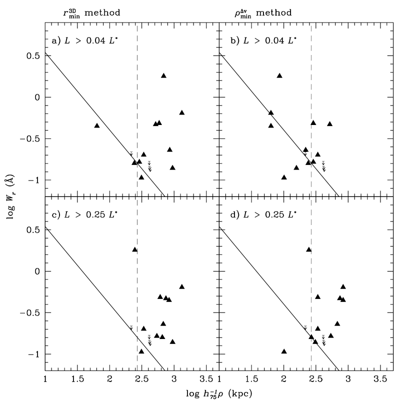
Figure 12: The rest equivalent width ($W_{r}$) vs. impact parameter ($\rho$) distribution is plotted for the two pairing methods, with the upper panels corresponding to the $L\geq 0.04L^{*}$ galaxy counterparts, and the lower panels to the $L\geq 0.25L^{*}$ galaxy counterparts. The solid line is the anticorrelation relation from Chen et al. (1998), and the dotted line demarks that group’s $\rho=270$${h_{75}^{-1}}$ kpc “physical pair” limit. The triangles are the data from this paper, and the limit signs indicate the $3\sigma$ $W_{r}$ detection limits for $L^{*}$ or brighter galaxies falling near the lines of sight that have no absorber within $\Delta v=300$ km s^-1.

One of the strongest pieces of evidence to associate Ly$\alpha$ absorbers with individual luminous galaxies is claimed to be the observed anticorrelation between rest equivalent width and impact parameter ( e.g. Tripp, Lu, & Savage (1998), CLWB ). In Figure 12, we plot impact parameter, $\rho$, of the galaxy vs. rest equivalent width, $W_{r}$, of the absorber. The top two panels (a & b) show the absorbers when matched to galaxies $L\geq 0.04L^{*}$, for the two methods, $r^{3D}_{min}$ and $\rho^{\Delta v}_{min}$, respectively, and the lower two panels (c & d) show the same for pairs matched to $L\geq 0.25L^{*}$ galaxies. Our identified absorbers are indicated by triangles, and the bright galaxies ($L>L^{*}$) with no detected absorption within $\Delta v=300$ km s^-1are shown as upper limits in equivalent width. The anticorrelation relationship from CLWB is also plotted as the solid line, and with that group’s “physical pair” limit of $\rho=270$${h_{75}^{-1}}$ kpc designated by the dashed line.

We note that for both pairing methods, the upper panels which include fainter galaxy counterparts appear consistent with the anticorrelation line, whereas the lower panels of brighter galaxies are not. This is interesting because the galaxies originally used to fit the function, from CLWB , only extend to $0.25L^{*}$ (with 3/35 exceptions, 2 of which are at the lowest redshifts). If our sample is similarly limited to $L\geq 0.25L^{*}$, as can be seen in Figures 12c and 12d, for a given $W_{r}$ line, we identify absorbers with galaxies at impact parameters much larger than the anticorrelation of CLWB would predict.

Removing the magnitude restrictions, our absorbers are invariably identified with fainter galaxies at smaller impact parameters for both pairing methods (seen in Figures 12a and 12b). To some degree, this can be expected for randomly distributed absorbers, which in all of our earlier random trials chose galaxies in the more luminous galaxy sample at typically larger impact parameters than in the fainter sample. However, it is difficult to disentangle such random effects from the real physical association of the absorbers and galaxies. CLWB define a model where the absorption is caused by an extended gaseous halo around the galaxy, and so a “physical pair” is an galaxy-absorber pair for which the galaxy-absorber cross-correlation function is greater than 1, and $\rho<270$${h_{75}^{-1}}$ kpc (Lanzetta et al. (1998)). In this scenario, the $W_{r}$–$\rho$ anticorrelation naturally arises for $\rho<270$ kpc, and an absorber associated with a galaxy at $\rho>270$ ${h_{75}^{-1}}$ kpc is caused by an undetected galaxy at smaller impact parameter that is correlated with the detected galaxy. In panels a and b of Figure 12, 2/11 and 7/11 of our absorbers fall within $\rho<$  270${h_{75}^{-1}}$ kpc, respectively, although some of these galaxies still fall at impact parameters too large for such low luminosity galaxies. The remaining pairs fall above this limit, which according to CLWB means these galaxies are correlated with undetected (i.e. lower luminosity) galaxies at smaller impact parameter. If this physical picture is correct, then roughly one-third to half of our absorbers are caused by galaxies somehow overlooked in our sample or by galaxies falling below $0.04L^{*}$.

Combining data from the literature on the $W_{r}$–$\rho$ anticorrelation in Figure 13, we see that all data sets mostly find galaxy-absorber pairs at the highest impact parameters, with the exception of CLWB which only find pairs for $\rho\lesssim$  270${h_{75}^{-1}}$ kpc, by construction. Here again we plot log $W_{r}$ vs. $\rho$  with the solid line indicating the CLWB best-fit and the large triangles are the data from the $\rho^{\Delta v}_{min}$ method from this paper. The open triangles are the galaxy-absorber pairs when matching only to $L\geq 0.25L^{*}$ galaxies, the filled triangles are the pairs when matching to $L\geq 0.04L^{*}$  galaxies, and the dotted line connects the galaxy data points for the same absorber. The other data included are from the literature, with filled symbols indicating galaxies with $L<0.25L^{*}$ and open symbols galaxies with $L>0.25L^{*}$.

At high $\rho$, there is no measurable anticorrelation between $W_{r}$ and $\rho$. At high $\rho$, it is easy to select a bright galaxy counterpart when there is in fact a fainter counterpart at smaller $\rho$, as observed for about half of our absorbers. However, of all the $L>0.25L^{*}$ points plotted, 8/11 from this paper, 4/5 from Morris et al. (1993), 5/5 from Tripp, Lu, & Savage (1998), and 0/3 from CLWB fall at $\rho>270$${h_{75}^{-1}}$ kpc, which is too large to be caused by an extended halo of such low luminosity galaxies. With the CLWB points removed, Figure 13 would resemble more of a scatter plot. As pointed out by Tripp et al. (1998), there are a number of $W_{r}>0.3$Å absorbers from CLWB sample with no counterpart galaxies, which could be associated with galaxies beyond their search radius. If those absorbers fall at large $\rho$, the anticorrelation would be further weakened.

Another feature of Figure 13 is upward trend of the $\rho\lesssim 200$${h_{75}^{-1}}$ kpc ($\simeq 160h_{100}^{-1}$ kpc) points, while the $\rho\gtrsim 200$${h_{75}^{-1}}$ kpc points show no real trend with $W_{r}$. This division has been suggested as an equivalent width effect ( c.f. Stocke et al. (1995)), with weaker lines arising from a different physical process. However, the division in Figure 13 does not correspond to any hard equivalent width cutoff, but could correspond to the $W_{r}$,$\rho$ position of a predominant transition in gas phase as calculated from simulation (Davé et al. (1998); see the next section of the paper.)

In framing our data in the context of the current literature, we have discovered significant problems with uniquely assigning an individual galaxy as associated with an absorber. In comparing two pairing methods ( $r^{3D}_{min}$ and $\rho^{\Delta v}_{min}$), which produce very different galaxy-absorber pairings, we find there is no way to statistically distinguish between the two methods as to which is a better prescription. Furthermore, each method is also very sensitive to magnitude completeness, since for three different absolute magnitude limits, we could almost always find a fainter galaxy at smaller impact parameters (an effect predicted by Linder (1998)). This is of particular concern for high redshift Ly$\alpha$ work, since the largest and brightest galaxies tell a different story than going further down the luminosity function. Moreover, these selection effects in luminosity do not address further ambiguities due to surface brightness selection effects (c.f. Rauch, Weymann, & Morris (1996)). Our $\sim 60$% covering factor for $L>0.25L^{*}$ galaxies is consistent with previous estimates, but, contrary to some predictions, yields smaller covering factors for fainter limits. This is contrary to expectations (c.f. CLWB ) that by going to faint enough magnitudes, every absorber can be reasonably associated with a galaxy. Limiting our data to galaxy-absorber pairs of limiting magnitude similar to those in the literature ($L>0.25L^{*}$), our data show no anticorrelation between $W_{r}$ and $\rho$. Extending that limit to intrinsically fainter galaxies does induce a $W_{r}$–$\rho$ correlation, but these fainter galaxies have correspondingly smaller halo sizes. Nothing in our data would specifically lead us to associate Ly$\alpha$ absorbers preferentially with luminous galaxies on halo size scales.

6 SUMMARY

The observation of low column density hydrogen absorbers has emerged as a powerful cosmological tool. Insights from theory and hydrodynamic simulations give the basic picture: the Ly$\alpha$ forest at high redshift is the main repository of baryons in the universe and it is a relatively unbiased tracer of the underlying dark matter distribution (Rauch 1998). Diffuse and highly ionized hydrogen forms a “cosmic web” of large scale structure (Bond & Wadsley 1998). As the universe expands and evolves, much of the gas is heated and shocked or collapses into galaxies and larger structures. The number density of absorbers declines toward low redshift, and they can only be studied from space. However, at low redshift it is possible to make direct comparisons with the galaxy distribution.

We have studied Ly$\alpha$ absorption along ten sightlines in the direction of the Virgo cluster. The resulting sample of 139 lines above a detection limit of 3$\sigma$ is the largest yet studied in the local universe ($z\lesssim 0.2$). At the resolution of the GHRS observations (200 km s^-1), essentially all of the absorption lines are unresolved. The number density of lines above a rest equivalent width of 0.24 Å, $dN/dz=38.3\pm 5.3$, agrees well with the the measurement from the Quasar Absorption Line Key Project (Weymann et al. 1998). There is marginal evidence for cosmic variance in the number of absorbers detected among the ten sightlines. Down to a limit of 0.1 Å, the line statistics are consistent with the study of two sightlines by Tripp et al. (1998) and with an extrapolation of the relationship for $dN/dW$ fitted to the Key Project data. The upturn in line density to $dN/dz=250\pm 40$ above 0.020 Å observed by Shull (1997) must set in at column densities below 10¹³ cm^-2.

We looked for clustering among the Ly$\alpha$ absorbers by carefully modelling the varying sensitivity and redshift pathlength of the ten different sightlines. Resolution and potential blending effects prohibit a search for clustering on velocity scales less than 250 km s^-1. We detect an excess of nearest neighbor line pairs on velocity scales of 250-750 km s^-1 at a 95-98% confidence level. There is no significant excess on larger scales that might correspond to the velocity dispersion of a rich cluster. The hypothesis that the absorbers are randomly distributed in velocity space can be ruled out at the 99.8% confidence level. No two-point correlation power is detected ($\xi<1$ with 95% confidence), in marginal disagreement with Tripp et al. (1998). We do not have the resolution or line statistics to look for the small scale clustering signal predicted by Cen et al. (1998). We find Ly$\alpha$ absorbers to be less clustered than bright galaxies, in accord with Grogin & Geller (1998). Absorber-absorber correlation amplitude on scales of 250-500 km s^-1 is 4–5 times smaller than galaxy-galaxy correlation amplitude.

A detailed comparison between absorbers and nearby galaxies produces results that are difficult to interpret. We restrict the comparison to the eleven Ly$\alpha$ lines in the radial velocity range 900–3000 km s^-1. Over the contiguous volume threaded by the ten sightlines, the galaxy sample is complete to $M_{B}=-16$. Absorbers lie preferentially in regions of intermediate galaxy density. It is not possible to uniquely assign a galaxy counterpart to each absorber, even if it is assumed that galaxies are surrounded by spherical halos that can cause absorption (CLWB). Ambiguities arise due to the uncertain mapping of redshift into distance and due to the large number of low luminosity galaxies for every luminous galaxy. We find multiple or non-unique absorber counterparts in 7/11 cases. The complete galaxy sampling allows us to do the converse experiment — to look for absorbers at small impact parameters from luminous galaxies. A halo covering factor to Ly$\alpha$ absorption of 20% is deduced for galaxies of $L>L^{*}$ and impact parameters $\rho<500$ kpc. For somewhat fainter galaxies, $L>0.25L^{*}$, with $\rho<270$ kpc, the covering factor is 60%. In general, there is no behavior in this sample that specifically implicates luminous galaxy halos in causing the absorption.

Some insight into the physical state of the absorbers at low redshift comes from a comparison with the recent hydrodynamic simulations of Davé et al. (1998; see also Reidiger et al. 1988; Theuns et al. 1998). They found that the dynamical state of an absorber — expanding or collapsing, shocked or unshocked — depends mainly on the overdensity of the gas, $\rho_{gas}/\bar{\rho}_{gas}$. With decreasing redshift and universal expansion, a given column density selects absorbers which are increasingly overdense and which have progressively more advanced dynamical states. Figure 14$a$ shows the rest equivalent width distribution of our sample of absorbers. In Figure 14$b$, the column density is estimated from rest equivalent width using a curve of growth and assuming a Doppler parameter of $b=30$ km s^-1. The vertical dashed line marks the column density below which the metal abundance of the absorbers falls sharply (Lu et al. 1998). We can use the relation between gas overdensity and column density from the simulations (in a $\Lambda$-dominated CDM model) to estimate the overdensity of our absorbers, as shown in Figure 14c (the conversion is relatively insensitive to the assumed Doppler parameter). The association of overdensity with the phase of the gas — diffuse IGM, shocked IGM, or condensed — is crude, because we have no estimate of the temperature of the gas and an increasing fraction of the moderate overdensity gas is shocked at decreasing redshift.

Because only the weakest lines in the sample have equivalent widths and overdensities that correspond to overdensities of a few, we infer that we are not in general probing the diffuse IGM. Tracing the evolution of the most diffuse structures from redshifts 3, 2, 1 and 0 means examining absorbers with column densities of $\log N_{HI}\approx 14.5$, 13.8, 13.2 and 12.7, respectively. For $b=30$ km s^-1 this corresponds to rest equivalent widths of about 0.39, 0.21, 0.075, and 0.026 Å. Possibly the sharp rise in $dN/dW$ seen by Shull (1997) below 10¹³ cm^-2 represents this intergalactic population. Most of the absorbers in the Virgo sample have overdensities ranging from a few up to $\sim 100$ and have not yet collapsed into galaxies.

Figure 15 revisits the distribution of equivalent width and galaxy impact parameter for our data (circled) and other studies in the literature. The approximate regions of the three absorbing gas phases are superimposed (Davé et al. 1998). An anticorrelation between $W_{r}$ and $\rho$ is anticipated because of the way gas traces the underlying mass distribution of large-scale structure. The strongest absorbers arise from the denser gas near galaxies, the majority of absorbers with 30${h_{75}^{-1}}$ $\lesssim\rho\lesssim$ 270${h_{75}^{-1}}$ kpc arise from shock-heated gas near galaxies, and absorbers with $\rho\gtrsim$ 270${h_{75}^{-1}}$ kpc are associated with a cooler, diffuse gas component. We cannot be sure that the segregation of observations to the upper regions of this plot is physically meaningful, since we have found ambiguities in the assignation of absorber counterparts, and some absorbers identified with luminous galaxies at large impact parameters might just as well be identified with lower luminosity galaxies at smaller impact parameters. The galaxy counterparts to our limited sub-sample of absorbers with radial velocities of 900–3000 km s^-1 are all at $\rho\gtrsim 70$${h_{75}^{-1}}$ kpc, too far to be bound to a halo potential. Our detection of weak clustering of the absorbers is consistent with gas that loosely traces large scale structure.

This study, and all others to this point, have been limited by the meager statistics of absorbers at low redshift. Future observations will allow us to increase the number of sightlines and revisit the issue of clustering. It will be very interesting to study the relation between clustering amplitude and gas overdensity. It may even be possible to identify a set of local absorbers at low column density that are primeval and completely unrelated to the space distribution of bright galaxies. We also plan to make direct comparisons between observations and hydrodynamic simulations, aiming to use Ly$\alpha$ absorbers for cosmological tests of increasing sophistication.

Figure 1: Spectra of the 12 quasars in the sample are displayed with the fitted continua (which omits the region near the geocoronal Ly$\alpha$ line) overplotted. Absorption lines are indicated with tickmarks and are numbered every two or three depending on the line density. Each panel is labelled with the quasar name and its emission redshift. Flux is plotted on the y-axis in units of $10^{13}\ \rm ergs\ s^{-1}cm^{-2}\AA^{-1}$

Figure 2: The 4.5$\sigma$ detection limit (rest equivalent width) for each spectum over the wavelength range corresponding to $0.003<z<0.225$ is shown by the solid curve. The dotted line indicates the 4.5$\sigma$ completeness level of 0.24 Å used by Jannuzi et al. (1998). The tickmarks show the location of Ly$\alpha$ absorbers.

Figure 3: The number of absorbers per interval redshift for each of the lines of sight individually. As seen in Figure 4, the average value agrees closely with Weymann et al. (1998), although two lines of sight differ by more than two standard deviations.

Figure 4: The number of Ly$\alpha$ absorption lines per redshift interval as a function of completeness limit. The solid line is the fitted distribution from the Quasar Absorption Line Key Project (Weymann et al. 1998), and the dashed lines are computed using the $1\sigma$ errorbars in $\gamma$ and $(dN/dz)_{0}$. The dotted lines represent the highest sensitivity of each GHRS spectrum. The solid symbols are values quoted for each of the studies made as noted in the legend. The open symbols are values quoted for some subset of the samples in each study, as described in the text.

Figure 5: (a) The observed nearest neighbor distribution is shown in the heavy solid line. The mean distribution expected from a random distribution of absorbers is shown by the solid line. The dotted and dashed lines indicate the 68%, 95% and 99% confidence intervals on the random distribution. Note that the strongest departures from a random distribution are the two lowest velocity bins not affected by resolution. (b) The distribution of the variance of the mean expected distribution and the expected distribution for each realization. The dotted line shows the variance of the observed and mean expected distributions. This implies the observed distribution has a small probability ($\leq 1$%) of having been drawn from a random velocity distribution.

Figure 6: The two-point velocity correlation function for the Ly$\alpha$ absorbers. The dotted and dashed lines are the 68% and 95% confidence intervals for a random distribution of absorbers. The black dots are the two-point correlation function for galaxies (Davis & Peebles 1983) Data for the smallest bin ($<250$ km s^-1) is omitted because of resolution limitations in the Ly$\alpha$ sample.

Figure 7: Luminosity function of Virgo sample of galaxies, spanning $600<v<3000$ km s^-1, plotted in log($\Phi\cdot$ Volume), or counts/magnitude. The error bars are Poisson. The curve is a Schechter luminosity function using average values for the Local universe of $M_{B}^{*}=-20$, $\alpha=-1.0$, and arbitrarily normalized to fit the turnoff.

Figure 8: Pieplot distributions of galaxies in Virgo sample out to $v=3000$ km s^-1. Quasar lines of sight are plotted as lines with absorbers indicated as circles. The larger circles are $4.5\sigma$ lines, and the smaller circles are $3\sigma$ lines. Each pieplot collapses $\sim 8$° in declination, spanning ranges (a) 11° to 19°, (b) 4° to 11°, and (c) $-$4° to 4°.

Figure 9: The one-dimensional galaxy distribution within impact parameters, $\rho$, of 1 Mpc from the individual quasar lines of sight are shown as the unshaded histogram. The shaded histogram is the galaxy distribution for $\rho\leq 250$${h_{75}^{-1}}$ kpc. The absorbers are indicated by the vertical bars, with the longer bars for $4.5\sigma$ lines, and shorter bars for $3\sigma$ lines.

Figure 10: The distributions of galaxy densities around the real absorber positions (darker histogram), compared to the galaxy densities around artificial absorbers (lighter histogram). Galaxy densities are calculated in 2${h_{75}^{-1}}$ Mpc spheres, assuming pure Hubble flow. Each histogram was individually normalized to the total number of absorbers, and the random absorbers are presented for the sum of 50 trials.

Figure 11: The distributions of impact parameters of the galaxy counterparts for the different galaxy-absorber pairing methods are plotted, with the darkly shaded histogram denoting the real absorbers and the lighter histogram the random absorbers. The left-most panels, (a) & (c), are the pairings for the $r_{min}^{3D}$ method, and the right-most panels, (b) & (d), are for the $\rho_{min}^{\Delta v}$ method. The upper panel absorbers are matched to $L\geq 0.04L^{*}$ galaxies, and the lower to $L\geq L^{*}$ galaxies. The number of pairs is normalized to total number for each test, and the random absorbers are presented for the sum of 50 trials.

Figure 13: The $W_{r}$ vs. $\rho$ data from this paper are plotted with data from the literature. Again, the solid line indicates the Chen et al. (1998) best-fit and the large triangles are the data from the $\rho_{min}^{\Delta v}$ method from this paper. The open triangles are the galaxy-absorber pairs when matching only to $L\geq 0.25L^{*}$  galaxies, the filled triangles are the pairs when matching to $L\geq 0.04L^{*}$  galaxies, and the dotted line connects the galaxy data points for the same absorber. The other data included are from Chen et al. (1998) [circles], Morris et al. (1993) [squares], Tripp et al. (1998) [3-pointed stars], and Le Brun et al. (1996) [5-pointed stars], with filled symbols indicating galaxies with $L<0.25L^{*}$ and open symbols galaxies with $L\geq 0.25L^{*}$.

Figure 14: (a) The distribution of rest equivalent widths for the 139 Ly$\alpha$ absorbers. The dashed line indicates the completeness limit used by the Quasar Absorption Line Key Project (Weymann et al. 1998). (b) The distribution of column densities obtained from the equivalent widths assuming a Doppler parameter of 30 km s^-1 and unresolved lines. The dashed line indicates the column density below which the metallicity of the absorbers falls sharply. (c) The distribution of gas overdensities ($\rho_{gas}/\bar{\rho}_{gas}$) estimated from the column density using the relation from Fig. 10 of Davé et al. (1998). The bars show the approximate dynamical state of the gas.

Figure 15: Same as Figure 13, with the sum of all the data from the literature plus the $L\geq 0.25L^{*}$ pairs from this paper indicated uniformly as triangles. The data from this paper is also circled. The shaded area defines the approximate region that the simulations of Davé et al. (1998) would populate on this diagram for the galaxies they associate with low column density Ly$\alpha$ absorbers in a $z=0,~{}\Lambda$-CDM universe. The line is their best fit, and the two vertical lines roughly denote the impact parameters at which the predominant phase of the absorbing gas changes from cold, condensed gas (smallest $\rho$), to shock heated gas (intermediate $\rho$), to diffuse gas (high $\rho$).

References

- Aldcroft (1993) Aldcroft, T. 1993, Ph.D. thesis, Stanford University
- Bahcall et al. (1993) Bahcall, J.N., et al. 1993, ApJS, 87, 1
- Bahcall et al. (1996) Bahcall, J.N., et al. 1996, ApJ, 457, 19
- Bahcall et al. (1992) Bahcall, J. N., Jannuzi, B.T., Schneider, D.P., Hartig, G.F., & Green, R.F. 1992, ApJ, 397, 68
- Bi & Davidsen (1997) Bi, H.G., & Davidsen, A. 1997, ApJ, 479, 523
- Binggeli, Popescu, & Tammann (1993) Binggeli, B., Popescu, C.C., & Tammann, G.A. 1993, A&AS, 98, 275
- Binggeli, Sandage, & Tammann (1985) Binggeli, B., Sandage, A., & Tammann, G.A. 1985, AJ, 90, 1681
- Blades, Turnshek & Norman (1988) Blades, J.C., Turnshek, D., & Norman, C.A. 1988, eds. Quasar Absorption Lines: Probing the Universe (Cambridge: Cambridge University Press)
- Bond & Wadsley (1998) Bond, J.R., & Wadsley, J.W. 1998, in Computational Astrophysics, ASP Conference Series Vol. 123, eds. D. Clarke & M. West, p. 323
- Bowen, Blades & Pettini (1996) Bowen, D.V., Blades, J.C., & Pettini, M. 1996, ApJ, 464, 141
- Cen et al. (1994) Cen, R., Miralda-Escudé, J., Ostriker, J.P., & Rauch, M. 1994, ApJ, 437, 9
- Cen et al. (1998) Cen, R., Phelps, S., Miralda-Escudé, J., & Ostriker, J.P. 1998, ApJ, 496, 577
- Cen & Simcoe (1997) Cen, R., & Simcoe, R.A. 1997, ApJ, 483, 8
- (14) Chen, H.-W., Lanzetta, K.M., Webb, J.K., & Barcons, X. 1998, ApJ, 498, 77 (CLWB)
- Cowie et al. (1995) Cowie, L.L., Songaila, A., Kim, T.-S., & Hu, E.M. 1995, AJ, 109, 1522
- Cristiani et al. (1997) Cristiani, S., D’Odorico, S., D’Odorico, V., Fontana, A., Giallongo, E., & Savaglio, S. 1997, MNRAS, 285, 209
- Croft et al. (1998) Croft, R.A.C., Weinberg, D.A., Katz, N., & Hernquist, L. 1998, ApJ, 495, 44
- Davé et al. (1998) Davé, R., Hernquist, L., Katz, N., & Weinberg, D.H. 1998, astro-ph/9807177
- Davé et al. (1997) Davé, R., Hernquist, L.H., Weinberg, D.H., & Katz, N. 1997, ApJ, 477, 21
- Davis & Peebles (1983) Davis, M., Peebles, P.J.E. 1983, ApJ, 267, 465
- de Vaucouleurs et al. (1991) de Vaucouleurs, G., de Vaucouleurs, A., Corwin Jr., H.G., Buta, R.J. Paturel, G., & Fouque, P. 1991, Third Reference Catalogue of Bright Galaxies, v.3.9 (RC3)
- Dinshaw et al. (1998) Dinshaw, N., Foltz, C.B., Impey, C.D., & Weymann, R.J. 1998, ApJ, 494, 567
- Dinshaw et al. (1995) Dinshaw, N., Foltz, C.B., Impey, C.D., Weymann, R.J., & Morris, S.L. 1995, Nature, 373, 223
- Dobrzycki & Bechtold (1997) Dobrzycki, A., & Bechtold, J. 1997, in Structure and Evolution of the Intergalactic Medium from QSO Absorption Line Systems, eds. P. Petitjean & S. Charlot (Paris: Editions Frontieres), p. 390
- Fang et al. (1996) Fang, Y., Duncan, R.C., Crotts, A.P.S., & Bechtold, J. 1996, ApJ, 462, 77
- Flint & Impey (1996) Flint, K.P., & Impey, C.D. 1996, AJ, 112, 865
- Fukugita, Okamura, & Yasuda (1993) Fukugita, M., Okamura, S., & Yasuda, N. 1993, ApJ, 412, L13
- Garcia et al. (1992) Garcia, A.M., Bottinelli, L.,Garnier, R., Gouguenheim, L., & Paturel, G. 1992, A&AS, 96, 435
- Gilliland (1994) Gilliland, R.L. 1994, GHRS Instrument Science Report #063, Space Telescope Science Institute
- Giovanelli (1997) Giovanelli, R. 1997, Private Communication to NED
- Giovanelli, Avera, & Karachentsev (1997) Giovanelli, R., Avera, E., & Karachentsev, I.D. 1997, AJ, 114, 122
- Gnedin & Hui (1996) Gnedin, N.Y., & Hui, L. 1996, ApJ, 472, 73
- Grogin & Geller (1998) Grogin, N.A., & Geller, M.J. 1998, ApJ, 505, 506
- Grogin, Geller, & Huchra (1998) Grogin, N.A., Geller, M.J. & Huchra, J.P. 1998, ApJS, 119, 277
- Gunn & Peterson (1965) Gunn, J.E., & Peterson, B.A. 1965, ApJ, 142, 1633
- Heap et al. (1995) Heap, S. R. et al. 1995, PASP, 107, 871
- Hernquist et al. (1996) Hernquist, L.H., Katz, N., Weinberg, D.H., & Miralda-Escudé, J 1996, ApJ, 457, 51
- Hewett, Foltz & Chaffee (1995) Hewett, P.C., Foltz, C.B., & Chaffee, F.H. 1995, AJ, 109, 1498
- Hoffman, Lewis, & Salpeter (1995) Hoffman, G.L., Lewis, B.M., & Salpeter, E.E. 1995, ApJ, 441, 28
- Hu et al. (1995) Hu, E.M., Kim, T.-S., Cowie, L.L. Songaila, A., & Rauch, M. 1995, AJ, 110, 1526
- Huchra et al. (1992) Huchra, J., Geller, M., Clemens, C., Tokarz, S., & Michel, A. 1992, Bull. C.D.S. 41, 31 (ZCAT)
- Jannuzi (1997) Jannuzi, B. 1997, in Structure and Evolution of the Intergalactic Medium from QSO Absorption Line Systems, eds. P. Petitjean & S. Charlot (Paris: Editions Frontieres), p. 93
- Jannuzi et al. (1998) Jannuzi, B.T., et al. 1998, ApJS, 118, 1
- Kirkman & Tytler (1997) Kirkman, D., & Tytler, D. 1997, ApJ, 484, 672
- Lanning et al. (1997) Lanning, H. H., Soderblom, D. R., Gonnella, A. & Sherbert, L. 1997, GHRS Instrument Science Report #081, Space Telescope Science Institute
- Lanzetta et al. (1998) Lanzetta, K.M., Webb, J.K., & Barcons, X. 1998, in The Young Universe: Galaxy Formation and Evolution at Intermediate and High Redshift, ed. S. D’Odorico, A. Fontana, & E. Giallongo, ASP Conf. Series Vol. 146, p. 175
- Lanzetta et al. (1993) Lanzetta, K.M., Turnshek, D.A., & Sandoval, J. 1993, ApJS, 84, 109
- Lanzetta, et al. (1995) Lanzetta, K.M., Bowen, D.V., Tytler, D., & Webb, J.K. 1995, ApJ, 442, 538
- Le Brun, Bergeron, & Boissé (1996) Le Brun, V., Bergeron, J., & Boissé, P. 1996, A&A, 306, 691
- Le Brun & Bergeron (1998) Le Brun, V., & Bergeron, J. 1998, A&A, 332, 814
- Leitherer et al. (1994) Leitherer, C., Koratkar, A., Lupie, O., & Hulbert, S. 1994, GHRS Instrument Science Report (ISR) #068, Space Telescope Science Institute
- Linder (1998) Linder, S.M. 1998, ApJ, 495, 637
- Lockman & Savage (1995) Lockman, F.J., & Savage, B.D. 1995, ApJS, 97, 1
- Loveday et al. (1992) Loveday, J., Peterson, B.A., Efstathiou, G., & Maddox, S.J. 1992, ApJ, 390, 338
- Lu et al. (1998) Lu, L., Sargent, W.L.W., Barlow, T.A., & Rauch, M. 1998, astro-ph/9802189
- Lynds (1972) Lynds, C.R. 1970, in External Galaxies and Quasi-stellar Objects, IAU Symposium No. 44, ed. D.S. Evans (New York: Springer-Verlag), p. 127
- Miralda-Escudé et al. (1996) Miralda-Escudé, J., Cen, R., Ostriker, J.P., & Rauch, M. 1996, ApJ, 471, 582
- Mo & Morris (1994) Mo, H.J., & Morris, S.L. 1994, MNRAS, 269, 52
- Morris et al. (1993) Morris, S.L., Weymann, R.J., Dressler, A., McCarthy, P.J., Smith, B.A., Terrile, R.J., Giovanelli, R., & Irwin, M. 1993, ApJ, 419, 524
- Morton (1991) Morton, D.C., 1991, ApJS, 77, 119
- Morton, York, & Jenkins (1988) Morton, D.C., York, D.G., & Jenkins, E.B. 1988, ApJS, 68, 449
- Petitjean & Charlot (1997) Petitean, P. & Charlot, S. 1997, eds. Structure and Evolution of the Intergalactic Medium from QSO Absorption Line Systems (Paris: Editions Frontieres)
- Petry, Impey, & Foltz (1998) Petry, C.E., Impey, C.D., & Foltz, C.B. 1998, ApJ, 494, 64
- Rauch (1998) Rauch, M. 1998 ARA&A, 36, 267
- Rauch, Weymann, & Morris (1996) Rauch, M., Weymann, R.J., & Morris, S.L. 1996, ApJ, 458, 518
- Riediger, Petitjean & Mcket (1998) Reidiger, R., Petitjean, P., & Mcket, J.P. 1998, A&A, 329, 30
- Sargent et al. (1980) Sargent, W.L.W., Young, P.J., Boksenberg, A., & Tytler, D. 1980, ApJS, 42, 41
- Savage et al. (1993) Savage, B.D., et al. 1993, ApJ, 413, 116
- Savage & Sembach (1996) Savage, B.D., & Sembach, K.R. 1996, ARA&A, 34, 279
- Savage, Sembach & Lu (1997) Savage, B.D., Sembach, K.R., & Lu, L. 1997, AJ, 113, 2158
- Shull (1997) Shull, J.M. 1997, in Structure and Evolution of the Intergalactic Medium from QSO Absorption Line Systems, eds. P. Petitjean & S. Charlot (Paris: Editions Frontieres), p. 101
- Shull, Stocke, & Penton (1996) Shull, J.M., Stocke, J.T., & Penton, S. 1996, AJ, 111, 72
- Slinglend et al. (1998) Slinglend, K., Batuski, D., Miller, C., Haase, S., Michaud, K., & Hill, J.M. 1998, ApJS, 115, 1
- Stocke et al. (1995) Stocke, J.T., Shull, J.M., Penton, S., Donahue, M., & Carilli, C. 1995, ApJ, 451, 24
- Strauss (1995) Strauss, M. 1995, NSSDC, 7185, 0
- (76) Strauss, M.A., Huchra, J.P., Davis, M., Yahil, A., Fisher, K.B., & Tonry, J. 1992, ApJS, 83, 29
- Theuns, Leonard, & Efstathiou (1998) Theuns, T., Leonard, A., & Efstathiou, G. 1998, MNRAS, 297, 49
- Tonry & Davis (1981) Tonry, J.L., & Davis, M. 1981, ApJ, 246, 680
- Tripp, Lu, & Savage (1998) Tripp, T.M., Lu, L., & Savage, B.D. 1998, ApJ, 508, 200
- Tsvetkov & Bartunov (1993) Tsvetkov, D.Yu. & Bartunov, O.S. 1993, BICDS, 42, 17
- Tully & Shaya (1984) Tully, R.B. & Shaya, E.J. 1984, ApJ, 281, 31
- Tytler et al. (1995) Tytler, D., Fan, X.-M., Burles, S., Cottrell, L., Davis, C., Kirkman, D., & Zuo, L. 1995, in QSO Absorption Lines, ed. G. Meylan (Berlin: Springer Verlag), p. 289
- Ulmer (1996) Ulmer, A. 1996, ApJ, 473, 110
- Weymann & Foltz (1983) Weymann, R.J., & Foltz, C.B. 1983, ApJ, 272, 1
- Weymann et al. (1998) Weymann, R.J., et al. 1998, astro-ph/9806123
- Weymann et al. (1995) Weymann, R., Rauch, M., Williams, R., Morris, S., & Heap, S. 1995, ApJ, 438, 650
- Weymann et al. (1979) Weymann, R.J., Williams, R.E., Peterson, B.M., & Turnshek, D.A. 1979, ApJ, 234, 33
- Womble, Sargent & Lyons (1996) Womble, D.S., Sargent, W.L.W., & Lyons, R.S. 1996, in Cold Gas at High Redshift, eds. Bremer, M. et al. (Dordrecht: Kluwer), p. 249
- Véron-Cetty & Véron (1993) Véron-Cetty, M.-P. & Véron, P. 1993, A Catalogue of Quasars and Active Galactic Nuclei, 6th ed., ESO Scientific Report, No. 7
- Aldcroft (1993)
- Bahcall et al. (1992)
- Bahcall et al. (1993)
- (93)
- Davé et al. (1998)
- Davis & Peebles (1983)
- Grogin & Geller (1998)
- Hu et al. (1995)
- Huchra et al. (1992)
- Jannuzi et al. (1998)
- (100)
- Lanzetta et al. (1995)
- Le Brun et al. (1996)
- Loveday et al. (1992)