Cosmic Microwave Background Temperature and Polarization Anisotropy in Brans-Dicke Cosmology

Abstract

We develop a formalism for calculating cosmic microwave background (CMB) temperature and polarization anisotropies in cosmological models with Brans-Dicke gravity. We then modify publicly available Boltzmann codes to calculate numerically the temperature and polarization power spectra. Results are illustrated with a few representative models. Comparing with the general-relativistic model with the same cosmological parameters, both the amplitude and the width of the acoustic peaks are different in the Brans-Dicke models. We use a covariance-matrix calculation to investigate whether the effects of Brans-Dicke gravity are degenerate with those of variation in other cosmological parameters and to simultaneously determine whether forthcoming CMB maps might be able to distinguish Brans-Dicke and general-relativistic cosmology. Although the predicted power spectra for plausible Brans-Dicke models differ from those in general relativity only slightly, we find that MAP and/or the Planck Surveyor may in principle provide a test of Brans-Dicke theory that is competitive to solar-system tests. For example, if all other parameters except for the CMB normalization are fixed, a value of the Brans-Dicke parameter $\omega$ as large as 500 could be identified with MAP, and for Planck, values as large as $\omega\simeq 3000$ could be identified; these sensitivities are decreased roughly by a factor of 3 if we marginalize over the baryon density, Hubble constant, spectral index, and reionization optical depth. In more general scalar-tensor theories, $\omega$ may evolve with time, and in this case, the CMB probe would be complementary to that from solar-system tests.

I Introduction

The Jordan-Fierz-Brans-Dicke theory [1, 2, 3] (heretofore, we will call it Brans-Dicke theory for simplicity) is the simplest example of a scalar-tensor theory of gravity [4]. Recently, scalar-tensor theories have received renewed interest, because such theories are generic predictions of superstring theory [5] and other higher-dimensional gravity theories [6]. Furthermore, scalar-tensor theories have also found application in construction of inflationary models, including some models based on first-order phase transitions that evade the “graceful exit” problem [7, 8, 9, 10].

In Brans-Dicke theory, Newton’s constant becomes a function of space and time, and a new parameter $\omega$ is introduced. General relativity is recovered in the limit $\omega\rightarrow\infty$. Solar-system experiments using Viking ranging data [11] have constrained $\omega\geq 500$. Recent VLBI measurement of the time delay of millisecond pulsars may further raise this limit [12]. However, these experiments are all “weak-field” experiments and probe only a limited range of space and time. To effectively constrain more general scalar-tensor theories, one would also like to have “strong-field” experiments, such as that provided by the binary pulsar[11, 14]. It was also pointed out [13] that in cosmological models based on more general scalar-tensor theories (in which $\omega$ can vary), there is generally an attractor mechanism that drives $\omega$ to $\infty$ at late times. Thus, it is possible that gravity differed considerably from general relativity in the early Universe, even if general relativity seems to work well today. Big-bang nucleosynthesis [15, 16, 17] provides one test of gravity at early times.

With the advent of precise new cosmic microwave background (CMB) data, it is natural to inquire whether the CMB might be able to provide new tests of Brans-Dicke theory (or of more general scalar-tensor theories). The Microwave Anisotropy Probe (MAP) [18] (to be launched in Fall 2000) and Planck Surveyor [19] (to be launched in 2007) satellites as well as many ground-based and balloon-borne experiments will measure the CMB anisotropy with unprecedented precision, thus providing a wealth of information about the early Universe. The advantage of the CMB anisotropy is that it involves fairly simple linear physics and is thus very “clean”. Furthermore, the CMB anisotropy probes a different era of the cosmos. Thus, at least in principle one may see the presence of a scalar-tensor theory that has been driven by the attractor mechanism to the general-relativity limit in the current epoch [13].

The possibility of testing scalar-tensor gravity with CMB anisotropy has already been noted. For example, the original version of extended inflation [7] was ruled out because the bubbles formed during the phase transition would have produced CMB anisotropy larger than that observed unless the Brans-Dicke parameter $\omega$ was less than 30 [8].

The general behavior of cosmological perturbations in Brans-Dicke cosmology was studied analytically in Refs. [20, 21], but they did not consider realistic models. Peebles and Yu, in their pioneering study of CMB anisotropy [22], considered a more realistic model with Brans-Dicke gravity, and they showed how the difference in the expansion rate affects the photon transfer function. More recently, Liddle et al. [23] estimated that in Brans-Dicke theory, the epoch of radiation-matter equality is shifted,

$$\frac{a_{\rm eq}H_{\rm eq}}{a_{0}H_{0}}=219h\left(1+\frac{5.81}{\omega}+\frac{\ln h}{\omega}\right),$$ (1)

and this accordingly affects the scale at which the present-day matter power spectrum turns over.

In the particular case of cosmologies based on chaotic-inflation models, the production of fluctuations during inflation with scalar-tensor gravity has been studied in Refs. [24, 25, 26]. They concluded that isocurvature perturbations could be produced during inflation, but are in general negligible compared with the adiabatic perturbations. In some inflation models, the spectrum of density perturbations may be affected, and for scalar-tensor theories with variable $\omega$, the spectral index for primordial perturbations may change with scale. For example, in some Brans-Dicke inflationary models there is a slight tilt in the spectrum of density perturbations, and a limit on the variation of $\omega$ can be obtained from the COBE observation measurement of the spectral index [27], but only within the context of this very particular inflation model.

In this paper, we perform a complete calculation of the CMB anisotropy in the Brans-Dicke theory. To do this we modify a standard code for CMB anisotropy calculation [28] to accommodate Brans-Dicke theory. Our modified code may be used to calculate the anisotropy in any given cosmological model. Although our code can accommodate isocurvature perturbations as well, we present numerical results only for models with nearly scale-invariant spectra of primordial adiabatic perturbations for the following reasons: If acoustic peaks like those expected from adiabatic perturbations are observed, then it is plausible that we might understand structure formation well enough to use CMB anisotropy to look for tiny deviations from general relativity. If it appears that some more complicated physics gave rise to structure formation, then it is unlikely that the CMB will provide a precision tool to study gravity.

We limit ourselves here to the simplest scalar-tensor theory: i.e., the original Brans-Dicke theory, for which the Brans-Dicke parameter $\omega$ is fixed. We will leave the more general case with variable $\omega$ to future work. Likewise, we concentrate on flat CDM models, including those with a cosmological constant, but without hot dark matter.

This paper is organized as follows: In Section II, we develop the formalism for the calculation. In Section III, we study the behavior of the background cosmology and discuss the initial conditions for the perturbations in the Brans-Dicke field. Numerical results are presented in Section IV, and we also discuss the detectability of Brans-Dicke theory there. Section V then summarizes and concludes. We briefly describe the numerical implementation of the calculation in the Appendix. Throughout this paper, we use natural units, $c=\hbar=k_{B}=1$.

II Formalism

A Brans-Dicke Theory

The Lagrangian density for the Brans-Dicke theory is

$${\mathcal{L}}=\sqrt{-g}\left[-\Phi R+\frac{\omega}{\Phi}g^{\mu\nu}\partial_{\mu}\Phi\partial_{\nu}\Phi+L_{m}\right],$$ (2)

where $\Phi$ is the Brans-Dicke field, and $L_{m}$ is the Lagrangian density for the matter fields, whose equations of motion are not affected. For convenience, we also define a dimensionless field

$$\phi=G\Phi,$$ (3)

where $G$ is the Newtonian gravitational constant measured today.

The Einstein equations are generalized to

$$G_{\mu\nu} = \frac{8\pi}{\Phi}T_{\mu\nu}+\frac{\omega}{\Phi^{2}}(\Phi_{;\mu}\Phi_{;\nu}-\frac{1}{2}g_{\mu\nu}\Phi_{;\lambda}^{\;\;;\lambda})+\frac{1}{\Phi}(\Phi_{;\mu\nu}-g_{\mu\nu}\Box\Phi),$$ (4)

where $T_{\mu\nu}$ is the stress tensor for all matter except for the Brans-Dicke field. The equation of motion for $\Phi$ is

$$\Box\Phi=\frac{8\pi}{2\omega+3}T.$$ (5)

Here $T=T^{\mu}_{\;\mu}$ is the trace of the energy-momentum tensor.

B Background Cosmology

The unperturbed part of the metric in a flat universe can be written as

$$ds^{2}=a^{2}(\tau)(-d\tau^{2}+\gamma_{ij}dx^{i}dx^{j}).$$ (6)

where $a$ is a function of the conformal time $\tau$ only, and $\gamma_{ij}$ is the flat-space metric. The unperturbed stress-energy tensor has components

$$T^{0}_{\;0}=-\rho,\qquad T^{0}_{\;i}=0,\qquad T^{i}_{\;j}=p\gamma^{i}_{\;j},$$ (7)

in the comoving frame. The equations describing the background evolution are

$$\rho^{\prime}+3\frac{a^{\prime}}{a}(\rho+p)=0,$$ (8)

$$\left(\frac{a^{\prime}}{a}\right)^{2}=\frac{8\pi Ga^{2}}{3\phi}\rho+\frac{\omega}{6}\left(\frac{\phi^{\prime}}{\phi}\right)^{2}-\frac{a^{\prime}}{a}\frac{\phi^{\prime}}{\phi},$$ (9)

$$\phi^{\prime\prime}+2\frac{a^{\prime}}{a}\phi^{\prime}=\frac{8\pi Ga^{2}}{2\omega+3}(\rho-3p),$$ (10)

where the prime denotes derivative with respect to $\tau$, and $\rho$ and $p$ are the total density and pressure of the Universe, respectively. General relativity is recovered in the limits

$$\Phi^{\prime\prime}\to 0,\quad\Phi^{\prime}\to 0,\quad\omega\to\infty.$$ (11)

C Cosmological Perturbations

We can write the perturbed metric as

$$g_{\mu\nu}=a^{2}(\gamma_{\mu\nu}+h_{\mu\nu}),$$ (12)

where the perturbation $h_{\mu\nu}$ is a function of space and time. It will be easier for us to deal with the (spatial) Fourier components of $h_{\mu\nu}$, and to avoid cluttered notation, we will subsequently denote the Fourier components $\tilde{h}_{\mu\nu}({\bf k})$ simply by $h_{\mu\nu}$. We choose to work in synchronous gauge, so $h_{00}=h_{0i}=h_{i0}=0$, and the $h_{ij}$ can be expanded in tensor harmonics, which satisfy $\nabla^{2}{\mathbf{Q}}^{(m)}=-k^{2}{\mathbf{Q}}^{(m)}$ [29, 32],

$$h_{ij} = \sum_{m}2H^{(m)}_{L}Q^{(m)}\gamma_{ij}+2H^{(m)}_{T}Q^{(m)}_{ij},$$ (13)

$$\delta\phi = \sum_{m}\chi^{(m)}Q^{(m)},$$ (14)

where $Q^{(m)}$ and $Q^{(m)}_{ij}$ are scalar and tensor harmonics, respectively, and $m$ denotes the “angular momentum” of the perturbation. For simplicity, we will write

$$H_{L}^{(0)} = h_{L},\qquad H_{T}^{(0)}=h_{T},$$ (15)

$$H_{T}^{(1)} = h_{V},\qquad H_{T}^{2}=H.$$ (16)

For models with only scalar and tensor modes, $h_{V}=0$. Our $h_{L}$ and $h_{T}$ are simply related to the variables used in Ref. [30] by

$$h=6h_{L},\qquad\eta=-(h_{L}+h_{T}/3).$$ (17)

The perturbed stress energy tensor can also be broken up into scalar, vector, and tensor parts. Let us denote a cosmic fluid component (e.g., baryons, neutrinos, photons, cold dark matter, etc.) by index $f$. We then know that the stress-energy perturbations $\delta T_{i}^{\;j}$ are related to the perturbations $\delta\rho$ and $\delta p$ in the density and pressure, respectively, and to the velocities $v_{f}$ and anisotropic stress $\pi_{f}$ (see, e.g., Refs. [30, 32] for more details),

$$\delta T^{0}_{\;0} = -\sum_{f}\sum_{m}\delta\rho^{(m)}_{f}Q^{(m)},$$ (18)

$$\delta T^{0}_{\;i} = \sum_{f}\sum_{m}(\rho_{f}+p_{f})v_{f}^{(m)}Q_{i}^{(m)},$$ (19)

$$\delta T_{0}^{\;i} = -\sum_{f}\sum_{m}(\rho_{f}+p_{f})v_{f}^{(m)}Q^{(m)i},$$ (20)

$$\delta T^{i}_{\;j} = \sum_{f}\sum_{m}\delta p_{f}^{(m)}\gamma^{i}_{\;j}Q^{(m)}+p_{f}\pi_{f}^{(m)}Q^{(m)i}_{j}.$$ (21)

If we consider only scalar and tensor perturbations, then the perturbed Einstein and Brans-Dicke equations are

$$\chi^{\prime\prime}+2\frac{a^{\prime}}{a}\chi^{\prime}+k^{2}\chi+3h^{\prime}_{L}\phi^{\prime} = \frac{8\pi Ga^{2}}{2\omega+3}\sum_{f}\left(\delta\rho_{f}-3\delta p_{f}\right);$$ (22)

$$k^{2}\left(h_{L}+\frac{1}{3}h_{T}\right)+3\frac{a^{\prime}}{a}h_{L}^{\prime} = \frac{4\pi Ga^{2}}{\phi}\sum_{f}\rho_{f}\delta_{f}-\frac{3}{2}(\frac{a^{\prime}}{a})^{2}\frac{\chi}{\phi}-\frac{\omega{\phi^{\prime}}^{2}\chi}{4\phi^{3}}+\frac{\omega\phi^{\prime}\chi^{\prime}}{2\phi^{2}}$$ (24)

$$-\frac{1}{2}\left[k^{2}\frac{\chi}{\phi}+3h^{\prime}_{L}\frac{\phi^{\prime}}{\phi}+3\frac{a^{\prime}}{a}\frac{\chi}{\phi}\right];$$

$$h_{L}^{\prime}+\frac{1}{3}h_{T}^{\prime} = -\frac{4\pi Ga^{2}}{\phi}\sum_{f}(\rho_{f}+p_{f})\frac{v_{f}}{k}-\frac{\omega\phi^{\prime}\chi}{2\phi^{2}}-\frac{1}{\phi}\left(\chi^{\prime}-\frac{a^{\prime}}{a}\chi\right);$$ (25)

$$h_{T}^{\prime\prime}+2\frac{a^{\prime}}{a}h_{T}^{\prime}-k^{2}(h_{L}+\frac{1}{3}h_{T}) = \frac{8\pi a^{2}}{\phi}p\pi_{f}-h_{T}^{\prime}\frac{\phi^{\prime}}{\phi}+k^{2}\frac{\chi}{\phi};$$ (26)

$$H^{\prime\prime}+2\frac{a^{\prime}}{a}H^{\prime}+k^{2}H=\frac{8\pi Ga^{2}}{\phi}p_{f}\pi_{f}^{(2)}.$$ (27)

D Temperature and Polarization Anisotropies

With these equations, one can find the evolution of perturbations using standard cosmological perturbation theory; see e.g. Ref. [29]. The calculation of the CMB anisotropy runs in parallel to the one in the standard model detailed, e.g., in Refs. [30, 31, 32]. Here we summarize the procedure for such calculations.

A temperature map $T(\hat{\mathbf{n}})$ of the sky (as a function of position $\hat{\mathbf{n}}$ on the sky) can be expanded in spherical harmonics,

$${T(\hat{\mathbf{n}})\over T_{0}}=1+\sum_{lm}a^{\rm T}_{(lm)}Y_{(lm)}(\hat{\mathbf{n}}),$$ (28)

where the mode amplitudes are given by the inverse spherical-harmonic transform. Similarly, if we measure the Stokes parameters $Q(\hat{\mathbf{n}})$ and $U(\hat{\mathbf{n}})$ as a function of position on the sky, they can be assembled into a symmetric trace-free (STF) $2\times 2$ tensor [34],

$${\cal P}_{ab}(\hat{\mathbf{n}})={1\over 2}\left(\begin{array}[]{cc}\vphantom{1\over 2}Q(\hat{\mathbf{n}})&-U(\hat{\mathbf{n}})\sin\theta\\ -U(\hat{\mathbf{n}})\sin\theta&-Q(\hat{\mathbf{n}})\sin^{2}\theta\\ \end{array}\right),$$ (29)

which can then be be expanded [34],

$${{\cal P}_{ab}(\hat{\mathbf{n}})\over T_{0}}=\sum_{lm}\left[a_{(lm)}^{{\rm G}}Y_{(lm)ab}^{{\rm G}}(\hat{\mathbf{n}})+a_{(lm)}^{{\rm C}}Y_{(lm)ab}^{{\rm C}}(\hat{\mathbf{n}})\right],$$ (30)

where the tensor spherical harmonics $Y_{(lm)ab}^{\rm G}$ and $Y_{(lm)ab}^{\rm C}$ form a complete basis for the gradient and curl components of the tensor field, respectively, and the multipole coefficients, $a_{(lm)}^{{\rm G}}$ and $a_{(lm)}^{{\rm C}}$ can be obtained by inverse transforms.

Thus, a combined temperature/polarization map is specified completely by the three sets of coefficients, $a_{(lm)}^{\rm T}$, $a_{(lm)}^{\rm G}$, and $a_{(lm)}^{\rm C}$. The two-point statistics of the T/P map are specified completely by the six power spectra $C_{l}^{{\rm X}{\rm X}^{\prime}}$ defined by

$$\left\langle\left(a_{(l^{\prime}m^{\prime})}^{\rm X^{\prime}}\right)^{*}a_{(lm)}^{\rm X}\right\rangle=C_{l}^{{\rm XX}^{\prime}}\delta_{ll^{\prime}}\delta_{mm^{\prime}},$$ (31)

for ${\rm X},{\rm X}^{\prime}=\{{\rm T,G,C}\}$, and the angle brackets denote an ensemble average. Parity invariance demands that $C_{l}^{\rm TC}=C_{l}^{\rm GC}=0$. Therefore the statistics of the CMB temperature-polarization map are completely specified by the four sets of moments, $C_{l}^{\rm TT}$, $C_{l}^{\rm TG}$, $C_{l}^{\rm GG}$, and $C_{l}^{\rm CC}$. These correlation functions are related to the ones used by Seljak and Zaldarriaga [35] by $C^{\rm GG}_{l}=C_{El}/2$, $C^{\rm CC}_{l}=C_{Cl}/2$, $C^{\rm TG}_{l}=C_{Cl}/\sqrt{2}$, and our $C^{TT}_{l}$ is the same as their $C_{Tl}$.

We can calculate the $C_{l}$’s by convolving the initial metric perturbation power spectrum $P_{\psi}$ with the photon transfer function $\Delta_{l}(k,\tau_{0})$,

$$C_{l}^{\rm T} = (4\pi)^{2}\int k^{2}dkP_{\psi}(k)[\Delta_{Tl}(k)]^{2},$$ (32)

$$C_{l}^{\rm GG} = (4\pi)^{2}\int k^{2}dkP_{\psi}(k)[\Delta_{Gl}(k)]^{2},$$ (33)

$$C_{l}^{\rm TG} = (4\pi)^{2}\int k^{2}dkP_{\psi}(k)[\Delta_{Tl}\Delta^{(S)}_{Gl}].$$ (34)

The photon transfer functions $\Delta_{Xl}(k,\tau_{0})$ are obtained by integrating along the line of sight [31],

$$\Delta_{Tl}(k,\tau_{0}) = \int_{0}^{\tau_{0}}d\tau S_{T}(k,\tau)j_{l}[k(\tau_{0}-\tau)],$$ (35)

$$\Delta_{Gl}(k,\tau_{0}) = \sqrt{\frac{(l+2)!}{(l-2)!}}\int_{0}^{\tau_{0}}d\tau S_{G}(k,\tau)j_{l}[k(\tau_{0}-\tau)],$$ (36)

where $j_{l}(x)$ is the spherical Bessel function and $S_{T,G}(k,\tau)$ are the source functions describing the Thomson scattering of photons along the path, and

$$S_{T} = g\left(\Delta_{T0}+2\alpha^{\prime}+\frac{v_{b}^{\prime}}{k}+\frac{\Pi}{4}+\frac{3\Pi^{\prime\prime}}{4k^{2}}\right)+e^{-\kappa}(\eta^{\prime}+\alpha^{\prime\prime})$$ (38)

$$+g^{\prime}\left(\frac{v_{b}}{k}+\frac{3\Pi^{\prime}}{4k^{2}}\right)+\frac{3g^{\prime\prime}\Pi}{4k^{2}},$$

$$S_{G} = \frac{3g(\tau)\Pi(\tau,k)}{8(k\tau)^{2}},$$ (39)

$$\Pi = \Delta_{T2}+\Delta_{G2}+\Delta_{G0},$$ (40)

where $x=k(\tau_{0}-\tau)$ and $\alpha=(h^{\prime}+6\eta^{\prime})/2k^{2}$. The visibility function $g(\tau)$ is given by $g=e^{-\kappa}\kappa^{\prime}$, where $\kappa(\tau)$ is the optical depth from conformal time $\tau$ to the current epoch. In the Brans-Dicke theory, the derivatives of $\alpha$ are given by

$$\alpha^{\prime} = -\frac{1}{k^{2}}\frac{a^{\prime}}{a}\left(h^{\prime}+6\eta^{\prime}\right)+\eta-\frac{8\pi Ga^{2}}{\phi}\frac{p\pi_{f}}{k^{2}}+\frac{1}{2k^{2}}\left(h^{\prime}+6\eta^{\prime}\right)\frac{\phi^{\prime}}{\phi}-\frac{\chi}{\phi},$$ (41)

$$\alpha^{\prime\prime} = -2\left(\frac{a^{\prime}}{a}\right)^{\prime}\alpha-2\left(\frac{a^{\prime}}{a}\right)\alpha^{\prime}+\eta^{\prime}-\frac{3}{2k^{2}}\frac{8\pi G}{\phi}\left[a^{2}\left(\rho+p\right)\sigma\right]^{\prime}$$ (43)

$$+\frac{3}{2k^{2}}\frac{8\pi Ga^{2}}{\phi}\left(\rho+p\right)\sigma\frac{\phi^{\prime}}{\phi}-\alpha^{\prime}\frac{\phi^{\prime}}{\phi}+\alpha\left(\frac{\phi^{\prime}}{\phi}\right)^{\prime}-\left(\frac{\chi}{\phi}\right)^{\prime}.$$

For the initial conditions on the scalar-field perturbation, we consider only the simplest case with $\chi_{\rm init}=\chi^{\prime}_{\rm init}=0$. The initial conditions for the matter are the same as those in the GR case [30]. As perturbations in the metric grow, perturbations in the Brans-Dicke field will also grow as shown in Eq. (22). However, for the initial condition we have chosen, the Brans-Dicke perturbation is so small that it has little effect on CMB anisotropy. An alternative choice of initial conditions for the Brans-Dicke perturbation would probably yield the same numerical results, because any initial perturbations are damped during the radiation dominated era [c.f. Eq. (22)].

The numerical calculation is essentially carried out by replacing the general-relativistic perturbation equations in a publicly available code [28, 33] by those in Eqs. (24)–(27) and including the evolution equation (22) for the Brans-Dicke field. In practice, there are a number of numerical issues and subtleties that arise, and some of these are detailed in the Appendix.

We have chosen to work in the Jordan frame in which the equations for spacetime-metric perturbations are altered while the equations for the stress-energy perturbations are unchanged. We considered working in the Einstein frame, in which the metric-perturbation equations are unchanged, but found that the changes in the equations for the stress-energy tensor would be more difficult to implement numerically.

III Background Cosmology

Let us now consider the background cosmology, and the boundary conditions for the homogeneous component of the Brans-Dicke field $\Phi$ and its conformal-time derivative $\Phi^{\prime}$. We define the cosmic scale factor at the present epoch to be $a_{0}=1$. In general-relativistic cosmology, the initial condition for the scale factor is $a(\tau=0)=0$. The conformal age of the Universe can be obtained by integrating,

$$\int_{0}^{\tau_{0}}d\tau=\int_{0}^{1}da/a^{\prime}.$$ (44)

For Brans-Dicke cosmology, additional boundary conditions are required for $\phi$ and $\phi^{\prime}$. One of these is determined by the requirement that the gravitational constant be in agreement with that measured today. This fixes [3]

$$\phi=\frac{2\omega+4}{2\omega+3}$$ (45)

at the present epoch.

The cosmological solutions for Brans-Dicke theory have been studied extensively [20, 37, 38, 39]. The Brans-Dicke field has a stiff equation of state; it dominates the dynamics at early stages of the expansion. However, for the era which affects the CMB anisotropy, the Brans-Dicke field must be subdominant, or else the expansion rate at nucleosynthesis would have been very different. Therefore, for a qualitative understanding of the expansion, we can assume that the change in $\phi$ does not affect the dynamics, and estimate how $\phi$ varies by assuming the Universe expands as in the GR case.

FIG. 1.: The function $K_{1}(x)/x$ versus $x=m/T$ (increasing time).

The equation of motion for the $\phi$ field is given by Eq. (10). It is analogous to a damped oscillator with a variable friction force. The initial “velocity” $\phi^{\prime}$ is damped in a few Hubble times. Therefore, for most of the time concerned, $\phi$ would only vary slowly. The right-hand side of Eq. (10) is the “driving force” for the motion of $\phi$. It is proportional to $\rho-3p$. If $\rho-3p$ were to vanish during radiation domination, then the quantity $y\equiv a^{2}\phi^{\prime}$ would be constant. However, it does not vanish during the radiation dominated era; in fact it is greater, even though the ratio $(\rho-3p)/\rho$ is smaller. There are two kinds of contributions to $\rho-3p$. First, the non-relativistic matter, including both baryons and cold dark matter, always contributes. Second, if one massive relativistic particle is present, it always dominates. For one species of massive relativistic particles,

$$\rho-3p=\frac{g}{2\pi^{2}}\int_{0}^{\infty}\left(E(p)-\frac{p^{2}}{E(p)}\right)p^{2}f(p)dp,$$ (46)

where $f(p)$ is the distribution function. For example, for a Boltzmann gas with zero chemical potential, $f(p)=e^{-E/T}$, and the result can be expressed in modified Bessel functions,

$$\rho-3p=\frac{g}{2\pi^{2}m^{4}}\frac{K_{1}(m/T)}{m/T}.$$ (47)

Fig. 1 plots this function. As one can see, as $T\to\infty$, $m/T\to 0$, and this function rises rapidly.

In the present paper, we will not consider massive neutrinos. In a CDM model, the last decoupled massive relativistic particles are electrons and positrons. They annihilate below $T\approx m_{e}=0.511$ MeV. For the scale we are interested in, the main contribution comes from the cold dark matter, which scales as $\rho_{c}=\rho_{c0}a^{-3}$.

After $e^{+}e^{-}$ annihilation, in the radiation dominated era,

$$a\propto\tau,\quad\phi^{\prime}\approx c_{1}+c_{2}a^{-2},$$ (48)

and one can see that $\phi$ approaches a “terminal velocity” and the initial velocity quickly dies out. From $T\sim 0.5$ MeV to $T\sim 10$ eV (matter-radiation equality), the initial velocity of $\phi$ is suppressed by a factor of $10^{9}$, and this initial “velocity” is constrained by nucleosynthesis, so it cannot be too large. We estimate,

$$\frac{2\omega+3}{12}\left(\frac{\phi^{\prime}}{\phi}\right)^{2}<\left(\frac{a^{\prime}}{a}\right)^{2},$$ (49)

at the end of nucleosynthesis. We find that for all practical purposes, we can take

$$a^{2}\phi_{i}^{\prime}=0.$$ (50)

This is effectively the Brans-Dicke initial condition [3] proposed in their first paper.

FIG. 2.: The time evolution of the Brans-Dicke field $\phi$.

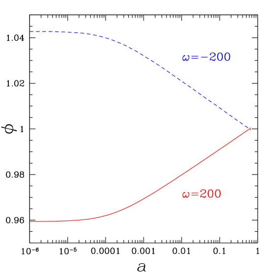
In the matter-dominated era, $\phi$ varies as $\phi\propto a^{1/(\omega+1)}$. For models with $\omega>0$, the value of $\phi$ increases with time, whereas for models with $\omega<0$, $\phi$ decreases with time. Fig. 2 shows the evolution of $\phi$.

We also note that in Brans-Dicke theory, the matter density is not precisely equal to the critical density in a flat Universe. The critical density in the Brans-Dicke theory depends on the parameter $\omega$. If we still define our relative densities in the usual way, i.e.,

$$\Omega_{i}=\rho_{i}/\rho_{c},\quad\rho_{c}=3H_{0}^{2}/8\pi G,$$ (51)

then we will have $\Omega=\sum_{i}\Omega_{i}\neq 1$ for flat geometry. Let us define

$$D\equiv\left(\frac{\phi^{\prime}}{\phi}\right)_{a=1};$$ (52)

then from Eq. (8) we have

$$\frac{\Omega}{\phi}=1+\frac{D}{H_{0}}-\frac{\omega}{6}\left(\frac{D}{H_{0}}\right)^{2}.$$ (53)

With the matching condition, $\phi=(2\omega+4)/(2\omega+3)$, one can obtain the value of $\Omega$ if $D$ is known. To proceed, one may start with some value of $\rho$ and solve the evolution equation to obtain $H_{0}$ and $D$. In practice, for the models considered here the difference is very small. We have tested for a few models with $\omega$ equal to a few hundred, and it does not make any significant difference.

FIG. 3.: CMB temperature/polarization power spectra for flat SCDM models in general relativity and in Brans-Dicke theories with $\omega=200$, $500$, and $-200$.

IV Results

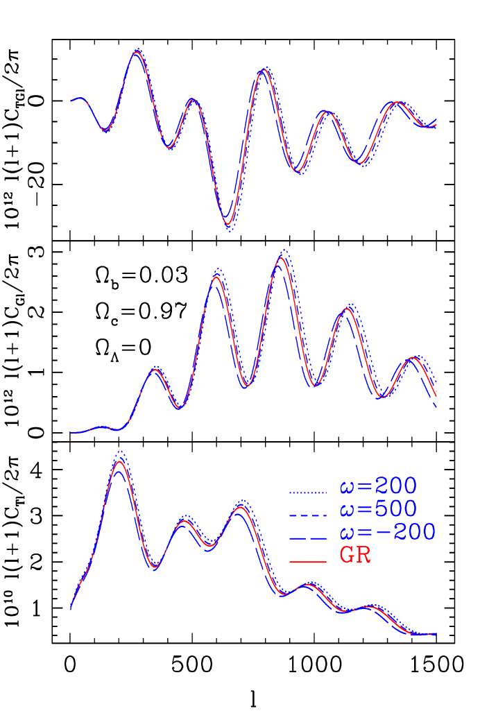
We now illustrate our numerical results with a few representative models. First we consider a COBE-normalized flat standard CDM (SCDM) model, with $\Omega_{b}=0.03$, $\Omega_{c}=0.97$ and $h=0.65$. The angular power spectra for $\omega=200$, 500, and $-200$ are plotted in Fig. 3 For comparison, we have also plotted the general-relativity result with the same physical parameters in the same plot.

For $\omega=\pm 200$ the difference between Brans-Dicke models and general relativity are clearly discernible As can be seen, both the normalization and width of the acoustic peaks are changed. The Brans-Dicke model with a positive $\omega$ has higher and broader acoustic peaks, while the negative-$\omega$ model has lower and narrower peaks. We have checked that the perturbations in the Brans-Dicke field near the time of decoupling in this model are very small. Thus, change in the acoustic-peak structure is due primarily to the change in the expansion rate near decoupling. For $\omega=500$ the difference is much less pronounced. The polarization spectra are similarly affected.

FIG. 4.: Spatial power spectra for SCDM models in Brans-Dicke theory with $\omega=200$ and $\omega=50$ and for general relativity.

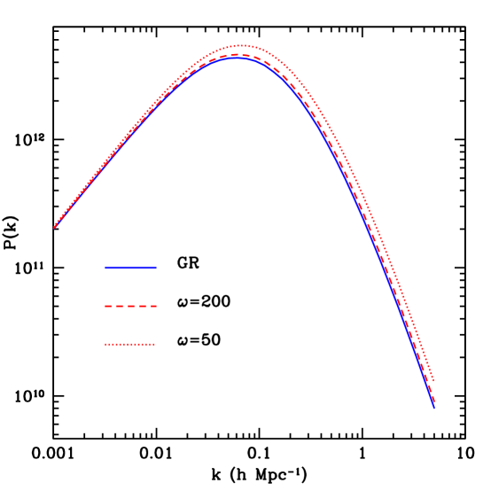
The Brans-Dicke field also affects the transfer function. Fig. 4 compares the matter transfer function in a general-relativity model, a Brans-Dicke model with $\omega=200$, and one with $\omega=50$. For the Brans-Dicke models, the bend of the matter power spectrum occurs at shorter wavelengths, and there is thus more small-scale power, in agreement with the claims of Ref. [23].

FIG. 5.: CMB power spectra for a Brans-Dicke SCDM model with $\Omega_{b}=0.03$ and $\omega=200$, and for general-relativistic models with $\Omega_{b}=0.3$ and $\Omega_{b}=0.032$.

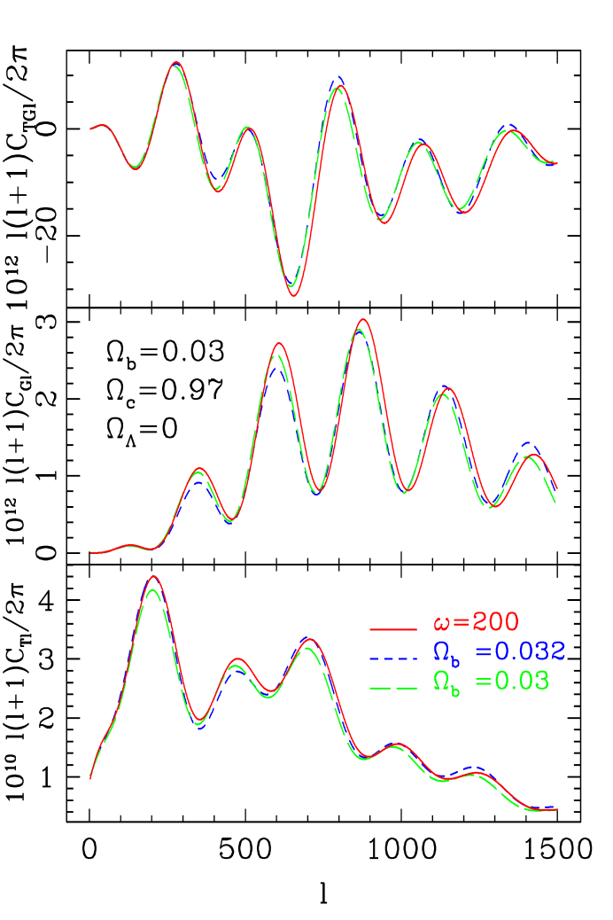
The CMB power spectra are also affected by other cosmological parameters, and it is possible that variation of some other parameters might mimic the effect Brans-Dicke gravity. For example, we plot the Brans-Dicke model with $\omega=200$ and $\Omega_{b}=0.030$ along with a general-relativity model with $\omega_{b}=0.032$ in Fig. 5. This general-relativity model mimics the Brans-Dicke model up to the first acoustic peak. Note, however, that this different $\Omega_{b}$ model does not fit the polarization better—in fact, the fit for the polarization is even worse. Therefore, observation of the polarization may help to lift this degeneracy of parameters.

It may also be possible to mimic the Brans-Dicke model entirely with a general-relativity model by adjusting more than one parameter. To investigate properly the possible degeneracy of the effect of varying $\omega$ with the possible effect of varying some combination of other cosmological parameters, we calculate the covariance matrix [40]. This also allows us to simultaneously estimate the precision with which $\omega$ (actually $\omega^{-1}$) can be recovered with a CMB map. We first consider only a temperature map and later consider the additional information that comes from the polarization. If the true parameters which describe the Universe are given by ${\mathbf{s}}_{0}$, then the Fisher information matrix is defined by

$$\alpha_{ij}=\sum_{l}\frac{1}{\sigma_{l}^{2}}\left[\frac{\partial C_{l}^{\rm TT}({\mathbf{s}}_{0})}{\partial s_{i}}\frac{\partial C_{l}^{\rm TT}({\mathbf{s}}_{0})}{\partial s_{j}}\right].$$ (54)

If the observed $C_{l}$’s are nearly Gaussian distributed around $C_{l}({\mathbf{s}}_{0})$ with variance $\sigma_{l}$, the covariance matrix $[{\mathcal{C}}]=[\alpha]^{-1}$ gives an estimate of the standard errors that would be obtained from a maximum-likelihood fit to the data. Approximately, the standard error with which the parameter $s_{i}$ could be obtained (after marginalizing over all other undetermined parameters) would be $\sigma_{s_{i}}={\mathcal{C}}^{1/2}_{ii}$.

Consider a CMB experiment that maps the temperature of the entire sky with a Gaussian beam of width $\theta_{\rm fwhm}$, with a noise per pixel of $\sigma_{\rm pix}$. If a fraction $f_{\rm sky}$ of the sky is used after a foreground cut, and the noise in each pixel is uncorrelated, then the the standard error with which each $C_{l}^{\rm TT}$ can be recovered is

$$\sigma_{l}=\left[\frac{2}{(2l+1)f_{\rm sky}}\right]^{1/2}\left(C_{l}+w_{T}^{-1}e^{l^{2}\sigma_{b}^{2}}\right),$$ (55)

where $\sigma_{b}=7.42\times 10^{-3}(\theta_{\rm fwhm}/1^{\circ})$, and the inverse weight $w_{T}^{-1}$ is given by

$$w_{T}^{-1}=4\pi\sigma^{2}_{\rm pix}/N_{\rm pix},$$ (56)

where $\sigma_{\rm pix}$ is the noise per pixel, and $N_{\rm pix}\simeq 40,000(\theta_{\rm fwhm})^{-2}$ is the number of pixels.

FIG. 6.: The largest finite value of $\omega$ that could be distinguished from infinity (i.e., general relativity) at the $2\sigma$ level as a function of the pixel noise of a given experiment that covers two-thirds of the sky. The fiducial model here is a standard CDM model (no cosmological constant). We show results for two beamwidths, $\theta_{\rm fwhm}=0.1^{\circ}$ and $\theta_{\rm fwhm}=0.3^{\circ}$. We assume here that $\Omega_{b}$, $h$, $n_{s}$, $\tau$, and $Q$ are marginalized over. The solid curve corresponds to $\theta_{\rm fwhm}=0.3^{\circ}$ with temperature data only, and the short dashed curve also includes the polarization. The long dashed curve corresponds to $\theta_{\rm fwhm}=0.1^{\circ}$with temperature data only, and the dotted curve includes also the polarization. The expected values of $\sigma_{\rm pix}$ for MAP and Planck are indicated.

FIG. 7.: Same as Fig. 6, except that all other parameters (except the normalization $Q$) are assumed to be known.

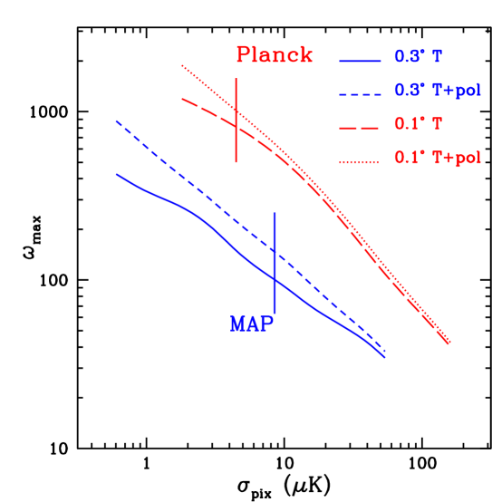
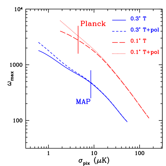
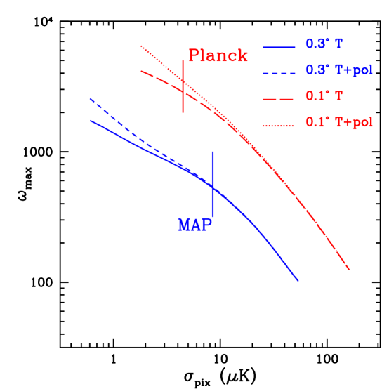
The goal of the MAP mission is to measure the temperature anisotropy with $\theta_{\rm fwhm}=0.3^{\circ}$ and $\sigma_{\rm pix}=20\,\mu{\rm K}$, which corresponds to $w_{T}^{-1}=2\times 10^{-15}$ (assuming a one-year experiment). The Planck Surveyor has a mission goal of $\theta_{\rm fwhm}=0.1^{\circ}$ and $\sigma_{\rm pix}=5\,\mu{\rm K}$, which corresponds to $w_{T}^{-1}=6\times 10^{-17}$. Assuming $f_{\rm sky}=0.67$, we calculate the Fisher information matrix with $\theta_{\rm fwhm}=0.3^{\circ}$ and $0.1^{\circ}$ for a variety of $w_{T}^{-1}$ values. The results are shown in Figs. 6 and 7. Our fiducial model is a COBE-normalized flat CDM model with $\{h_{0},\Omega_{b},n_{s},\tau,1/\omega,(Q/Q_{\rm COBE})^{2}\}=\{0.65,0.03,1,0.5,0,1\}$ where $n_{S}$ is the primordial power-spectrum index, $\tau$ the reionization optical depth, and $Q_{\rm COBE}(n_{s}=1)=18~{}\mu{\rm K}$ is the COBE normalization [42]. We assume 3 generations of massless neutrinos and no massive neutrinos, and consider scalar modes only. The derivatives of $C_{l}$ are calculated by varying each of the parameters by 0.5%. To calculate the partial derivatives of the $C_{l}$’s with respect to $1/\omega$, we compare the general-relativity model with a Brans-Dicke model with $\omega=200$. Our calculation sums up modes up to $l\leq 3000$. We have checked to make sure that our results are not sensitive to the step size for calculating the derivative nor the cutoff of $l$.

	$h_{0}$	$\Omega_{b}$	$n_{S}$	$\tau$	$(Q/Q_{\rm COBE})^{2}$	$1/\omega$
value	0.65	0.03	1.0	0.5	1	0
$\sigma_{\rm MAP}(T)$	0.045	0.0054	0.043	0.057	0.057	0.0050
$\sigma_{\rm MAP}(T+P)$	0.031	0.0036	0.031	0.035	0.053	0.0034
$\sigma_{\rm Planck}$	0.0045	0.00049	0.0081	0.013	0.018	0.00062
$\sigma_{\rm Planck}(T+P)$	0.0037	0.00040	0.0055	0.006	0.017	0.00049

TABLE I.: Error estimates for parameters of an SCDM model. Here, MAP is assumed to have $\theta_{\rm fwhm}=0.3^{\circ}$ and $w^{-1}=2\times 10^{-15}$; Planck is assumed to have $\theta_{\rm fwhm}=0.1^{\circ}$ and $w^{-1}=6.3\times 10^{-17}$.

The value of $\sigma_{1/\omega}$ depends on the number and uncertainty of other parameters. Table I lists the standard errors that could be obtained by marginalizing over all others for the various parameters we consider. Fig. 6 plots the smallest value of $\omega$ that could be distinguished from $\omega=\infty$ (i.e., general relativity) at the 95% confidence level. So, for example, if all the parameters listed above were unknown and had to be determined from CMB data alone, then the CMB would be marginally competitive with (current) solar-system tests; i.e., if we marginalize over $Q_{\rm COBE}$, $\Omega_{b}$, $h$, $n_{s}$, and $\tau$, then the smallest value of $\omega$ that could be distinguished from $\infty$ is $\simeq 100$ for MAP and $\simeq 800$ for the Planck Surveyor.

On the other hand, if we assume that all parameters except for $\omega$ and the normalization can be determined completely from other experiments, then the sensitivity to a finite $\omega$ can be improved, as also illustrated in Fig. 7. For example, a finite value of $\omega$ as large as $\omega\simeq 500$ could be detectable with MAP and $\simeq 2500$ for Planck.

The future satellite missions will measure not only the temperature anisotropy but also the polarization. It is possible to improve the accuracy of cosmological-parameter determination by combining the temperature and polarization data, as Fig. 5 illustrated that polarization may help break degeneracies in parameter space.

To include the polarization data, we generalize Eq. (54) to

$$\alpha_{ij}=\sum_{X,Y}\sum_{l}\left[\frac{\partial C_{X,l}}{\partial s_{i}}\left[\Xi^{-1}\right]_{X,Y}\frac{\partial C_{Y,l}}{\partial s_{j}}\right].$$ (57)

Here, $X,Y=$TT, GG, CC, TG, and $[\Xi^{-1}]_{X,Y}$ are elements of the inverse noise covariance matrix $\Xi$. The elements of $\Xi$ were given in Refs. [34, 35]. If the two linear-polarization states are given equal integration times, the total number of photons available for temperature measurement are twice of that for polarization measurement, thus

$$(\sigma_{\rm pix}^{T})^{2}=\frac{1}{2}(\sigma^{P}_{\rm pix})^{2}.$$ (58)

If the number of pixels are equal, then

$$w_{T}^{-1}=w_{P}^{-1}.$$ (59)

The results obtained from combining the temperature and polarization data are also plotted in Figs. 6 and 7, and these plots show that the sensitivity to the Brans-Dicke parameter $\omega$ could be further improved by including polarization. The effect is particularly strong when the effect of Brans-Dicke gravity is degenerate with that of variation of other cosmological parameters in a temperature map. By including the polarization data in MAP, the CMB should be sensitive to models with $\omega<150$ at 95% CL when all other parameters are undetermined, or $\omega<500$ when only CMB normalization is undetermined (in this case, there is not much gain from polarization). For Planck, these numbers are $\omega<1000$ and $\omega<3200$, respectively. On the other hand, if all the other parameters are known, the benefit gained from adding polarization measurement is less obvious; only for detectors with pixel noise less than $5\mu$K there is a difference.

FIG. 8.: CMB power spectra for $\Lambda$CDM models in Brans-Dicke theory with $\omega=200$ and in general relativity.

FIG. 9.: The same as Fig. 6, except that here we use a flat cosmological-constant model with a nonrelativistic-matter density $\Omega_{0}=0.4$.

FIG. 10.: Same as Fig. 9, except that all other parameters (except the normalization $Q$) are assumed to be known.

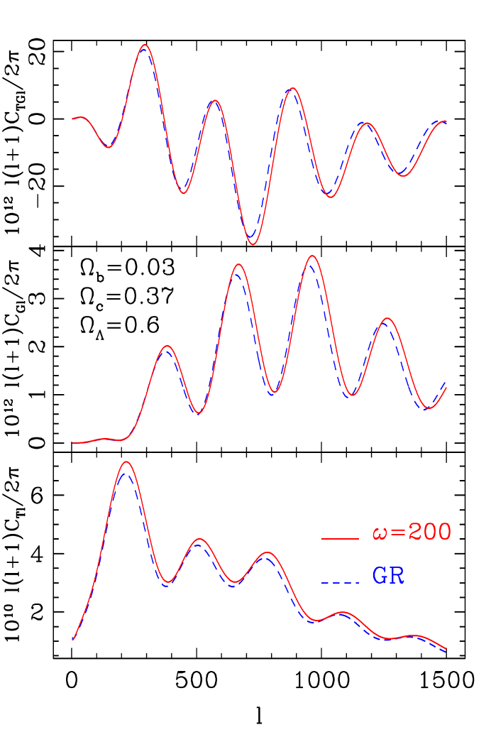
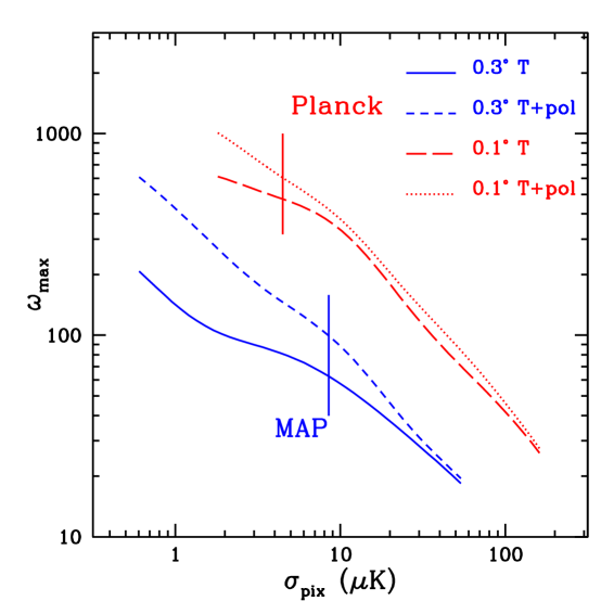
There has been much recent interest in models with a nonzero cosmological constant prompted, in particular, by the evidence for an accelerating universe from supernovae [43]. We have also performed our calculations for a $\Lambda$CDM model, and the results are shown in Fig. 8 for $\omega=200$. The results for the Fisher-matrix analysis are shown in Figs. 9 and 10, and they are similar to those in the SCDM case.

Finally, we have noted before, if $\omega$ is finite, then $\Omega$ is not precisely equal to unity [cf., Eq. (53)], and one might wonder whether the effects on the CMB power spectra of varying $\omega$ can be mimicked by varying $\Omega$. We have checked that for the Brans-Dicke models we have investigated, the change in the CMB power spectra is much too large to be attributed to this shift in $\Omega$.

V Conclusion and Summary

We have developed a formalism for calculating the CMB anisotropy in cosmological models with Brans-Dicke gravity. This was done by modifying standard Boltzmann codes for CMB power spectra. Because Brans-Dicke theory satisfies the medium-strong equivalence principle, only those equations determining the evolution of the metric need to be modified; the equations of motion for various matter or radiation components are the same as in general relativity. One boundary condition for the Brans-Dicke theory is determined by requiring $\phi=\frac{2\omega+4}{2\omega+3}$ at the current epoch. Another is given by adopting the Brans-Dicke initial condition $a^{2}\phi^{\prime}=0$ at early time (after the annihilation of electron-positron pairs).

This formalism is then used to calculate the CMB power spectra in several models. We find that in Brans-Dicke models, both the height and width of the acoustic peaks are changed. While there is some degeneracy with different cosmological parameters at low $l$ in a temperature map, we demonstrate that the effect can be distinguished by going to higher acoustic peaks and by observing the polarization of the CMB. Our results show that with high-quality CMB data, the CMB anisotropy may provide a powerful test for Brans-Dicke theory that is competitive (and complementary) to solar-system tests.

As an example, we examined a flat SCDM model. MAP temperature data should be able to distinguish Brans-Dicke gravity with $\omega<100$ from general relativity at the 95% CL if all other parameters must be simultaneously determined from the CMB, or $\omega<500$ if all other parameters except for the CMB normalization are fixed. With Planck, these numbers are $800$ and $2500$ respectively.

Furthermore, even better results are achievable if both temperature and polarization data are used. For MAP, the two limits are raised to $150$ and $800$, respectively, and for Planck, $1000$ and $3200$, respectively. We also examined the case of a flat $\Lambda$CDM model and found similar results.

In conclusion, the differences between the CMB power spectra expected in general relativity and those in Brans-Dicke models with acceptable values of $\omega$ are small. However, our Fisher-matrix analysis shows that if systematic effects can be controlled, then the CMB sensitivity (from Planck) to a finite value of $\omega$ might be competitive with that from solar-system tests. We re-emphasize that the CMB will provide a new and independent test of gravity in stronger fields and at earlier times. Thus, it is conceivable that the CMB will provide a unique test of some scalar-tensor theories in which $\omega$ would have been smaller at earlier times.

A Numerical Implementation

In this Appendix we briefly describe the numerical implementation of the calculation. First we consider the background evolution. The boundary conditions for the Brans-Dicke field $\phi$ are given in Eqs. (45) and (50). From Eq. (45), we know the end-point value of $\phi$ but not the initial value. We pick an arbitrary epoch with temperature 10 eV$\ll T\ll 0.5$ MeV, then pick some value of $\phi$ with $\phi^{\prime}=0$ and integrate forward until the scale factor $a=1$. This process is reiterated with different trial initial values of $\phi$ until the condition $\phi_{0}=(2\omega+4)/(2\omega+3)$ is satisfied to the required precision. Formally, the process is equivalent to numerical root finding, and we use a Brent algorithm [44] to find the root.

In the original CMBFAST code, any epoch in the evolution of the Universe is specified by the cosmic scale factor $a$, and the time $\tau$ is obtained by integrating Eq. (44). In Brans-Dicke theory, the value of $a^{\prime}/a$ is given by Eq. (9), and it is no longer convenient to use $a$ as the argument. Instead, we use $\tau$ to specify the cosmic time, and the scale factor $a$ is obtained by solving the whole set of background-evolution differential equations. This is done in the beginning of the calculation, and the values of $\{\tau,a(\tau),a^{\prime}(\tau),\phi(\tau),\phi^{\prime}(\tau)\}$ are then stored. Subsequently, given either $\tau$ or $a$, the whole set of these values corresponding to that epoch can be obtained by lookup and/or interpolation. The second-order derivatives $a^{\prime\prime}$ and $\phi^{\prime\prime}$ can also be obtained by numerical difference.

This more complicated implementation of the cosmic history also demands modification in other parts of the code. In the original code, the expansion rate is calculated from the density of the universe using the Friedman equation; in this new code, we replace it by interpolation from the stored data in all such cases.

For example, in the original code, the baryon temperature, ionization fraction, and baryon sound speed are given as a functions of $a$, and are calculated by a simple integration of the Friedmann equation. In the new scheme, this calculation is modified so that the value of $a^{\prime}$ is obtained by lookup or/and interpolation of the stored data. We also modified the code for the calculation of the baryon sound speed. In the original calculation, there are occasional jumps in the baryon sound speed, which may be due to the truncation error in calculating the derivative ${\rm d}T_{b}/{\rm d}\ln a$. We have modified the algorithm so that there is no jump in this calculation. However, our tests show that these occasional jumps do not have any significant effect on the end result, probably because only interpolated values are used, and the result is mostly important only in a limited range.

For the calculation of the perturbative part, we note that in Brans-Dicke theory, the equation of motion for the matter or radiation are the same as in general relativity. All we need to do is to replace the perturbed Einstein equations by Eqs. (22)–(27). Following the original code, we use Eq. (24) to force conservation of energy and reduce the numerical error in solving the ordinary differential equations. We have tested that when $\omega\to\infty$ we recover the general-relativistic result produced by the standard code.

Finally, the temperature and polarization anisotropy may be obtained by integrating Eqs. (32)–(34). The expression for the source function is the same, but note that there are Brans-Dicke corrections to the derivatives of metric perturbations as given in Eqs. (41)–(43), and these must be implemented in the code.

REFERENCES

- [1] P. Jordan, Nature (London) 164, 637 (1949); Schwerkraft und Weltall, Vieweg, Braunschweig, 1955; Z. Phys. 157, 112 (1959).
- [2] M. Fierz, Helv. Phys. Acta 19, 128 (1956).
- [3] C. Brans and R. H. Dicke, Phys. Rev. 124, 925 (1961); R. H. Dicke, Phys. Rev. 125, 2163 (1962); R. H. Dicke, Phys. Rev. 152, 1 (1968).
- [4] P. G. Bergmann, 1968, Int. J. Theor. Phys. 1, 25; K. Nordtvedt, Astrophys. J. 161, 1059 (1970); R. V. Wagoner, Phys. Rev. D 1, 3209 (1970); J. D. Bekenstein, Phys. Rev. D 15, 1458 (1977); J. D. Bekenstein and A. Meisels, Phys. Rev. D 18, 4378 (1978).
- [5] M. B. Green, J. H. Schwarz, and E. Witten, Superstring Theory (Cambridge University Press, Cambridge, 1987).
- [6] T. Appelquist, A. Chodos, and P. G. O. Freund, Modern Kaluza-Klein Theories (Addison-Wesley, Redwood City, 1987).
- [7] D. La and P. J. Steinhardt, Phys. Rev. Lett. 62, 376 (1989); Phys. Lett. B 220, 375 (1989).
- [8] E. J. Weinberg, Phys. Rev. D 40, 3950 (1989); D. La, P. J. Steinhardt, and E. W. Bertschinger, Phys. Lett. B 231, 231 (1989).
- [9] P. J. Steinhardt and F. S. Accetta, Phys. Rev. Lett. 64, 2740 (1990); J. D. Barrow and K. Maeda, Nucl. Phys. B 341, 1990 (1990); J. Garcia-Bellido and M. Quiros, Phys. Lett. B 243, 45 (1990); R. Holman, E. W. Kolb, and Y. Wang, Phys. Rev. Lett. 65, 17 (1990).
- [10] A. D. Linde, Phys. Lett. B 238, 160 (1990).
- [11] See e.g., C. Will, Theory and Experiment in gravitational Physics (Cambridge University Press, Cambridge, 1993), and references therein .
- [12] C. Will, gr-qc/9811036.
- [13] T. Damour and K. Nordtvedt, Phys. Rev. Lett. 70, 2217 (1993), Phys. Rev. D 48, 3436 (1993); J. Garcia-Bellido and D. Wands, Phys. Rev. D 52, 5636 (1995).
- [14] T. Damour and G. Esposito-Farese, Phys. Rev. D 54, 1474 (1996).
- [15] M. Kamionkowski and M. S. Turner, Phys. Rev. D 42, 3310 (1990).
- [16] J. A. Casas, J. Garcia-Bellido, and M. Quiros, Mod. Phys. Lett. A 7, 447 (1992); T. Damour and C. Gundlach, Phys. Rev. D 43, 3873 (1991).
- [17] T. Damour and B. Pichon, astro-ph/9807176.
- [18] MAP: http://map.gsfc.nasa.gov.
- [19] Planck: http://astro.estec.esa.nl/Planck.
- [20] H. Nariai, Prog. Theor. Phys. 42, 544 (1969).
- [21] J. P. Baptista, J. C. Fabris, and S. V. B. Goncalves, gr-qc/9603015.
- [22] P. J. E. Peebles and J. T. Yu, Astrophys. J. 162, 815 (1970).
- [23] A. R. Liddle, A. Mazumdar, and J. D. Barrow, Phys. Rev. D 58, 027302 (1998).
- [24] A. A. Starobinsky and J. Yokoyama, gr-qc/9502002.
- [25] J. Garcia-Bellido and D. Wands, Phys. Rev. D 52, 6739 (1995).
- [26] T. Chiba, N. Sugiyama, and J. Yokoyama, Nucl. Phys. B 530, 304 (1998).
- [27] C. L. Bennett et al., Astrophys. J. 464, L1 (1996); K. M. Gorski et al., ibid., L11; G. Hinshaw et al., ibid., L17.
- [28] http://www.sns.ias.edu/matiasz/CMBFAST/cmbfast.html.
- [29] H. Kodama and M. Sasaki, Prog. Theor. Phys. 78, 1 (1984).
- [30] C. P. Ma and E. Bertschinger, E. Astrophys. J. 455, 7 (1995).
- [31] U. Seljak and M. Zaldarriaga, Astrophys. J. 469, 437 (1996).
- [32] W. Hu, U. Seljak, M. White, and M. Zaldarriaga, Phys. Rev. D 57, 3290 (1998).
- [33] http://arcturus.mit.edu/cosmics/
- [34] M. Kamionkowski, A. Kosowsky, and A. Stebbins, Phys. Rev. D 55, 7368 (1997).
- [35] U. Seljak and M. Zaldarriaga, Phys. Rev. D 55, 2054 (1997).
- [36] M. Zaldarriaga, D. N. Spergel, and U. Seljak, Astrophys. J. 488, 1 (1997).
- [37] L. E. Gurevich, A. M. Finkelstein, and V. A. Ruban, Astrophys. Space Sci. 22, 231 (1973).
- [38] J. D. Barrow and P. Parsons, Phys. Rev. D 55, 1906 (1997).
- [39] D. J. Holden and D. Wands, Class. Quant. Grav. 15, 3271 (1998).
- [40] G. Jungman, M. Kamionkowski, A. Kosowsky, and D. N. Spergel, Phys. Rev. Lett. 76, 1007 (1996); Phys. Rev. D 54, 1332 (1996).
- [41] E. F. Bunn and M. White, Astrophys. J. 480, 1 (1997).
- [42] C. L. Bennett et al., ApJ19964641; K. M. Gorski et al., ApJ199646411.
- [43] S. Perlmutter et al., Nature (London) 391, 51 (1998); P. Garnavich et al., Astrophys. J. 507, 46 (1998); A. G. Riess et al., Astron. J. 116, 1009 (1998).
- [44] See, e.g., W. H. Press et al., Numerical Recipes in Fortran: The Art of Scientific Computing, 2nd ed., (Cambrige University Press, Cambridge, 1992).