Line profile analysis of the $\delta$ Scuti star HD 2724$\equiv$BB Phe: mode identification and amplitude variations

Abstract

The line profile variations of the $\delta$ Scuti star HD 2724$\equiv$BB Phe were studied on the basis of new 189 high–resolution spectrograms covering 52 hours of observations on a baseline of 8.3 days. By combining these results with those of a previous campaign 13 pulsation modes were identified: 5 of them are both photometric and spectroscopic, 3 are purely spectroscopic and 5 purely photometric. For the first time it was possible to compare spectroscopic data taken in two different seasons: 6 modes were found to be common to both datasets and furthermore strong amplitude variations of the excited modes were detected. The fit of the line profile variations with a model of non-radial pulsating star allowed us to obtain a reasonable estimate of the inclination of the rotational axis and to propose the $\ell,m$ typing of the spectroscopic modes. The frequency content resembles that of 4 CVn, a $\delta$ Sct star with similar physical parameters.

1 Introduction

The light and line profile variations of the $\delta$ Scuti star HD 2724$\equiv$BB Phe have been recently studied by Bossi et al. (1998, hereinafter Paper I). On the basis of 11 consecutive nights of photometric observations and 5 simultaneous consecutive nights of spectroscopic ones they detected 13 probable pulsation modes, 7 of which were determined in an unambiguous way. For 4 modes it was possible to suggest an identification of their $\ell$ and $m$ parameters; in particular, the proposed identification of the lowest frequency mode as the radial fundamental one allowed a more accurate refinement of the stellar physical parameters which were also consistent with the Hipparcos parallax.

Due to the relatively short spectroscopic baseline, some of the modes detected in Paper I had barely resolved frequencies; as a consequence, some ambiguities arose in their detection and in the successive attempts of their typing. With the aim to confirm and eventually improve these findings, an application for a longer run was submitted to ESO. In this paper we describe the results we obtained; unfortunately, in the meantime all the facilities for getting photometric data were dismissed and we had to limit ourselves to a purely spectroscopic campaign, to which 10 consecutive nights were allotted (October 1–11, 1997).

2 New spectroscopic observations and data processing

The spectroscopic observations were made at La Silla Observatory (ESO) with the Coudé Echelle Spectrometer attached to the Coudé Auxiliary Telescope. Owing to bad weather, it was possible to get useful observations during 8 nights only. The run was performed in Remote Control Mode from Garching headquarters; the CES was configured in the blue path with the long camera and the CCD #38. The resulting reciprocal dispersion was 0.018 Å pix^-1 with an effective resolution of about 54000. The useful spectral region ranges from 4482 to 4534 Å. The integration time was set to 15 minutes; a total of 189 useful spectrograms were collected covering about 52 hours of stellar monitoring on a baseline of 8.3 days. Data reduction was performed using the MIDAS package. The spectrograms were normalized by means of internal quartz lamp flat fields and calibrated into wavelengths by means of a thorium lamp.

Due to stellar projected rotational velocity, only the Feii line at 4508.4 Å is completely free from blends of adjacent features and allows a good normalization to the stellar continuum. Therefore, in the same way as we did in Paper I, we studied the behaviour of this line. All the spectrograms were averaged to obtain a very high $S/N$ average spectrum. It was then possible to select two windows on both sides of the Feii line. As a further step, the individual spectrograms were normalized to the continuum defined by a linear least–squares fit of these windows. Finally, the spectra were shifted and rebinned in order to remove the observer’s motion. In the rebinning procedure the spectrograms were resampled with a step of 0.04 Å  (average of 2 original pixels): in such a way we saved the effective resolution according to the Nyquist criterion and we improved the $S/N$ of the resulting profiles. The mean standard deviation of the pixels on the stellar continuum allowed us to estimate the $S/N$ of the spectrograms: the resulting average value at the continuum level is 368.

A non–linear least–squares fit of a rotationally broadened gaussian profile to the average line profile allowed us to estimate the projected rotational velocity and intrinsic width: $v\sin i=83.0\pm 1.0$ km s^-1 and $W_{i}=13.7\pm 0.5\leavevmode\nobreak\$km s^-1. This $v\sin i$ is in excellent agreement with the value of $82\pm 2$ km s^-1 derived in Paper I. Figure 1 shows the average profile obtained from the 1997 observations fitted with the computed rotationally broadened profile (dashed line).

Figure 1: Average profile of the Feii 4508Å line with the best fitting rotationally broadened profile superimposed ($v\sin\leavevmode\nobreak\ i=83.0$ km s^-1).

3 Analysis of line profile variations

3.1 The least–squares algorithm

The search for periodicities in the line profile variations was performed by using a generalized form of the least–squares power spectrum technique, originally developed for the study of monodimensional time series analysis by Vaniĉek (1971). Let $P(\lambda_{j},t_{k})$ the observed line profiles, $j$ the pixel number and $t_{k}$ the time of the $k$-th spectrogram. The global variance is defined by:

$$\sigma_{T}=\sum_{j,k}w_{k}^{2}(P(\lambda_{j},t_{k})-P_{0}(\lambda_{j}))^{2}$$

where $P_{0}(\lambda_{j})$ is the time averaged profile and $w_{k}$ are the normalized weights derived from the $S/N$ of the spectrograms. If we have already detected $m$ periodic sinusoidal components (“known constituents”) and if we are looking for the $(m+1)$-th component, we can explore the useful frequency range (0$<\nu_{i}<25$ cd^-1) by fitting each pixel time series $j$ with the series

$$p_{i,j}(t_{k})=\overline{p}_{i}+\sum_{l=1,m}A_{i,j,l}\cos(2\pi\nu_{l}t_{k}+\phi_{i,j,l})$$

$$+A_{i,j,m+1}\cos(2\pi\nu_{i}t_{k}+\phi_{i,j,m+1})$$

where $\overline{p}_{i},A_{i,j,l}$ and $\phi_{i,j,l}$ (with $1\leq l\leq m+1$) are the free parameters. Then we compute the global reduction of variance defined as

$$RF_{i}=1-\sum_{j,k}w_{k}^{2}(p_{i,j}(t_{k})-P(\lambda_{j},t_{k}))^{2}/\sigma_{m}$$

where $\sigma_{m}$ is the global residual variance after the fit of the line profile variations with the $m$ “known constituents”. The frequency $\nu_{i}$ giving the highest $RF$ (or one of its 1 cd^-1 aliases if there is a better agreement with the photometrically detected modes) is then selected as the $(m+1)$–th known constituent and the procedure is iterated again. At the end of this procedure, after having detected $M$ known constituents, we can perform a final fit of $P(\lambda_{j},t_{k})$ and derive the functions: $\overline{p}_{M}(\lambda_{j})$ (i.e. the best estimate of the unperturbed line profile), $A_{l}(\lambda_{j}),\phi_{l}(\lambda_{j})$ (with $1\leq l\leq M$) and also their formal errors.

3.2 Frequency identification in 1997 data

Following the procedure described above, 8 terms have been successively detected: 8.58, 8.05, 6.49, 0.07 (or 1.07), 5.74, 5.31, 7.38 and 6.99 cd^-1. Other smaller amplitude terms are probably present, but we cannot assign a frequency value in a reliable way. The detected modes are listed in Tab. 1 in order of increasing frequency (first column); the second column reports their rms amplitudes computed along the whole line profile and expressed in thousandths of the continuum amplitude.

Table 1: Amplitudes of the photometric and spectroscopic modes; values between brackets are uncertain (see text). The amplitude of the 6.99 cd^-1 term cannot be determined in the 1993 data owing to the low frequency resolution. Spectroscopic amplitudes are in units of the continuum intensity.

		Spectroscopy			Photometry
Freq.		1997	1993		$b$ light
[cd-1]		[10-3]	[10-3]		[mmag]
4.43		–	–		8.4
4.54		–	–		2.8
5.31		1.67	(3.43)		6.7
5.63		–	–		2.9
5.74		2.14	4.93		11.1
5.88		–	–		3.9
6.12		–	–		5.6
6.26		–	(5.22)		–
6.49		1.88	2.95		4.8
6.99		2.15	–		–
7.38		2.10	2.44		9.1
8.05		2.73	3.55		3.6
8.58		2.78	2.40		–

Frequency detection by means of the least–squares technique can seem a subjective procedure when dealing with single–site observations. As our experience on photometric data proves, this is not true: as an example, see the frequencies detected by Mantegazza et al. (1994) on the basis of single–site observations and their confirmation by Breger et al. (1995) on the basis of multisite ones. However, to give an independent confirmation of these results, we performed a second analysis by using the CLEAN algorithm generalized so as to analyse line profile variations (Mantegazza et al. 1999, in preparation). The averaged spectrum of the line profile variations is shown in Fig. 2.

Figure 2: CLEAN spectrum of the new data collected in 1997. The identified peaks are discussed in the text.

The only difference between the two algorithms is the value assigned to the low frequency term: 0.07 cd^-1 from the least–squares analysis and 1.07 cd^-1 from the CLEAN algorithm (of course, one term is an alias of the other). However, we do not assign great significance to this peak: given its closeness to the value of the sidereal day it is probably an artifact due to observation and/or reduction procedures. In particular, during the reductions it has been observed that a slight rotation of the spectrograms on the CCD occurred during the night; this could be responsible for this low frequency term. Therefore, this term will not be considered any more in the following. All the other terms detected independently by the two techniques are coincident.

Figure 3: Amplitudes and phases of the modes detected by the least-squares power spectrum analysis in the 1997 data. All the diagrams have the same scales: amplitudes are in units of the continuum intensity (each tick corresponds to 0.001) and phases are in degrees (each tick corresponds to 50^o).

3.3 Comparison with the 1993 results

In the third column of Tab. 1 we list the rms amplitudes of the terms detected from the 1993 spectrograms. These values were obtained by including in the least–squares fit both the 5.31 and the 6.26 cd^-1terms. Owing to the fact that they are barely resolved, their amplitudes are rather uncertain. Furthermore, the amplitudes of the other terms can change by up to about 20% or so according to whether one term or both are considered in the fit. Notwithstanding these uncertainties it is quite evident that, comparing the 1993 and the 1997 data, the amplitudes of the other terms have decreased, with the only exception of the 8.58 cd^-1 term which shows the opposite behaviour. For the modes detected in the 1993 photometric data, we have reported their $b$–light amplitude in the fourth column of Tab. 1.

We see that there is a substantial agreement in the frequency detection between the two seasons: only one mode was detected in 1993 but not in 1997 (6.26 cd^-1) and only one in 1997 but not in 1993 (6.99 cd^-1). The probable reality of the 6.26 cd^-1 term was already discussed in Paper I, taking also into account its relative closeness to the 1 cd^-1 alias of the 5.31 cd^-1term.

The 6.99 cd^-1 term was not detected in the 1993 data probably because it was drowned in the 7.05 cd^-1 alias of the strongest spectroscopic mode (8.05 cd^-1). In fact, in 1993 data the peak at 7.05 cd^-1was the highest one, probably owing to the 6.99 cd^-1contribution. The correct value (8.05 cd^-1) was deduced with the help of the photometry. The resolution of the 1997 data is sufficient enough to detect the 6.99 cd^-1term: as a matter of fact the least–squares analysis finds this term both considering a term at 7.05 or at 8.05 cd^-1.

In summary, five terms were detected in the two spectroscopic datasets and in the photometric one: 5.736, 5.311, 6.488, 8.049 and 7.382 cd^-1 . The 6.26, 6.99 and 8.58 cd^-1 are purely spectroscopic terms, while the 4.430, 4.536, 5.629, 5.877 and 6.123 cd^-1 ones are only photometric. Even if the detection of these terms in the three different time series (especially in the spectroscopic ones) was not an easy task, we obtained a well–defined picture of the pulsational content of HD 2724 as a final result. In particular, we had for the first time the possibility to compare two spectroscopic solutions obtained in different years.

The amplitudes of modes are changed, as it can be seen comparing the different columns of Tab. 1 where we list the average amplitudes along the line profile of the identified modes in the two observing seasons (cols. 2 and 3).

3.4 Phase diagrams of spectroscopic terms

Figure 3 shows the amplitude and phase diagrams of the behaviour along the line profile of the detected modes (i.e. the functions $A_{l}(\lambda_{j}),\phi_{l}(\lambda_{j}),1\leq l\leq 7$ previously described). For the sake of clarity only the points with a formal error bar smaller than $40^{o}$ are shown in the phase panels.

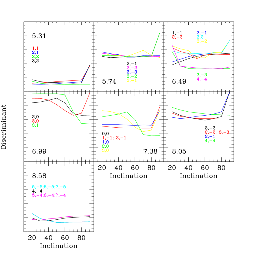
Figure 4: Discriminants of the best fitting modes for the spectroscopically detected terms vs. the inclination of rotational axis (in degrees). $\ell,m$ numbers are in the same colour of the corresponding line.

Table 2: Identification of the pulsation modes. Inclination angle was assumed to be 70^o. With respect to Paper I, the identification of the 5.31 cd^-1 term is changed and the 6.99 cd^-1 term was not previously detected.

Term		Mode typing
[cd-1]		($\ell,m$)
5.31		$(2,2)\leavevmode\nobreak\ \leavevmode\nobreak\ (2,1)\leavevmode\nobreak\ \leavevmode\nobreak\ (1,1)\leavevmode\nobreak\ \leavevmode\nobreak\ (3,2)$
5.74		$(2,-2)\leavevmode\nobreak\ \leavevmode\nobreak\ (2,-1)$
6.49		$(1,-1)\leavevmode\nobreak\ \leavevmode\nobreak\ (2,-1)\leavevmode\nobreak\ \leavevmode\nobreak\ (2,-2)$
6.99		$(3,1)\leavevmode\nobreak\ \leavevmode\nobreak\ (2,0)\leavevmode\nobreak\ \leavevmode\nobreak\ (3,0)$
7.38		$(1,-1)\leavevmode\nobreak\ \leavevmode\nobreak\ (2,-1)\leavevmode\nobreak\ \leavevmode\nobreak\ (0,0)\leavevmode\nobreak\ \leavevmode\nobreak\ (1,0)$
8.05		$(4,-4)\leavevmode\nobreak\ \leavevmode\nobreak\ (3,-3)\leavevmode\nobreak\ \leavevmode\nobreak\ (3,-2)$
8.58		$(5,-5)\leavevmode\nobreak\ \leavevmode\nobreak\ (6,-5)\leavevmode\nobreak\ \leavevmode\nobreak\ (7,-5)$

The behaviours of the phase diagrams are similar for the modes detected in the two seasons, with only a notable exception concerning the 5.31 cd^-1 term. In the analysis of the 1993 data the reality of the 6.26 cd^-1 term was established, but this term is not very prominent in the 1997 data, because meanwhile its amplitude may have decreased. However, this dataset has a better frequency resolution and the 5.31 and 6.26 cd^-1 terms could be well resolved. Hence, we can obtain a more clear phase diagram of the 5.31 cd^-1 term: we verified that the phase increases with the wavelength, although we stated the opposite behaviour in Paper I. We performed several tests on the 1993 data and we definitely established that the mode identification proposed in Paper I suffers from the interference between one term and the alias at $\pm$ 1 cd^-1 of the other term (in particular the 5.31 cd^-1 term was affected by the alias at 5.26 cd^-1 of the 6.26 cd^-1 term). We therefore believe that the most reliable solution should be the one derived from the new data and that the mode identification proposed in the next subsection is more reliable than the one reported in Paper I.

Among the other phase diagrams the cleanest is that of the 8.58 cd^-1 term, which clearly indicates that it is a relatively high–degree prograde mode, in agreement with the results of Paper I.

3.5 Mode typing

An attempt to identify the modes can be accomplished by fitting the line profile variations with the technique already described in Paper I. In the case of the present data, we are forced to fit the line profile variations only without the simultaneous light variations; this makes it difficult to introduce the flux (or temperature) variations in the model. Of course, without this constraint, the model obtained from the 1997 data is a little less well defined, but in spite of that we could obtain important statements on the pulsational content. Therefore, we limited ourselves to considering the vertical velocity ($v_{r}$) and its phase as the only free parameters of the model, while the horizontal velocity $v_{h}$ was kept linked to $v_{r}$ by the usual relationships $v_{h}=74.4Q^{2}v_{r}$ ($Q$: pulsational constant) and we assumed the same phase for both. These approximations are legitimated by the fact that $v_{h}<<v_{r}$. Finally, no flux variations were allowed. The other parameters were the same as in Paper I, in particular the stellar physical parameters.

We explored all the possible combinations of $\ell,m$ up to $\ell=4$ and inclination angles between 20^o (at this inclination the rotational velocity is close to the stellar break–up velocity) and 90^o. For the highest $S/N$ term (8.58 cd^-1 ) term we extended the search to $\ell=7$, because its phase diagram clearly indicated that it could be a relatively high–degree mode.

The discriminants of the best fitting modes are reported for each term in the panels of Fig. 4 as a function of the inclination angle. It should be noted that in each phase diagram we show only the plausible solutions, i.e. those giving a low value for the discriminant. The solutions yielding unacceptable values are omitted for the sake of clarity. As an example of the quality of the fits supplied by this technique, Fig. 5 shows the variations of the line profile due to the 8.58 cd^-1 term phased on a complete cycle and the corresponding best fitting variations produced by a model of a nonradial mode with $\ell=6,m=-5$ and assuming $i=70^{o}$. As can be seen from Fig. 4 we can be reasonably sure that the 8.58 cd^-1 is a mode with $\ell=6\pm 1$ and $m=-5$: unfortunately, we cannot be more precise since the discriminants of these three modes are practically coincident.

By examining Fig. 4 we see that the results are not very clear in the sense that for most of the terms different modes give equivalent fits at different inclinations. However, the 6.99 cd^-1 mode seems to be slightly in favour of a solution with a high inclination (say $i\geq 60^{o}$). In Paper I we left an uncertainty on two possible values for the inclination angle, i.e. $50^{o}$ or $70^{o}$. On the basis of the new results, we prefer the latter; however, most of the proposed mode identifications are plausible also for the former value.

Owing to the fact that more than one identification is possible for the same term, the identifications suggested in Paper I are generally agreed on. The strongest disagreement is about the 5.31 cd^-1 term, which should be prograde or axissymmetric according to the old data while the new ones indicates clearly that it is retrograde. The reason for this discrepancy has been already discussed when dealing with the phase diagrams. According to that discussion we have to be more confident in the results obtained from 1997 data.

We report in Tab. 2 the identifications which are compatible both with the present data and with the 1993 ones. In particular, some possible identifications suggested by Fig. 4 have been rejected (as for example the 3,–3 and 4,–4 couples for the 6.49 cd^-1) because they are unable to fit the light variations observed in 1993.

As regards the 8.05 cd^-1 term, our calculations show that the local flux of a (4,-4) mode varies of about 0.3 mag and that of a (3,-3) mode of about 0.15 mag. The cancellation effect reduces it to the observed mmag level.

Figure 5: The variations induced on the line profile by the 8.58 cd^-1term phased over 1 cycle (continuous line) and the best–fitting model of a mode with $\ell=6$,$m=-5$ and $i=70^{o}$ (dashed lines). The small bar at the lower left indicates a 0.005 amplitude in continuum intensity units.

4 Conclusions

The new set of spectrograms of HD 2724 has allowed to confirm the detection of the modes found in the 1993 data and a new mode has been detected at 6.99 cd^-1. There is evidence that the amplitudes of the modes have considerably changed, in particular the 8.58 cd^-1 term, which was among the weakest in 1993, is now the strongest. Amplitude variations are well established in $\delta$ Sct stars thanks to extensive photometric studies. A a matter of fact, HD 2724 is the first star in which these variations are also observed spectroscopically. In particular, it should be emphasized that the 6.26 cd^-1 term, clearly detected in the 1993 data, was not recovered in the 1997 ones.

As regards the frequency content, HD 2724 is very similar to 4 CVn (Breger & Hiesberger 1999). At least 7 frequencies (5.88, 6.12, 6.26, 6.49, 6.99, 7.38 and 8.58 cd^-1 in HD 2724; 5.85, 6.12, 6.19, 6.44, 6.98, 7.38 and 8.59 cd^-1 in 4 CVn) have almost the same value. Among the high–amplitude terms in 4 CVn, only the 5.05 cd^-1 term has no correspondance in HD 2724. The physical parameters of the two stars are similar: T_eff=6900$\pm$100 K, $\log g$=3.4$\pm$0.1, $v\sin i$=73 km s^-1 for 4 CVn (Breger et al. 1990), 7200$\pm$100 K, 3.44$\pm$0.03, 83 km s^-1 for HD 2724 (Paper I). HD 2724 does not show the cross–coupling terms found in the 4 CVn light curve, but this can be due to the smaller amplitude of the modes excited in HD 2724. On the basis of this similarity, the comparison between the frequency content of $\delta$ Sct stars deserves further attention in the future.

The mode typing has been partially hampered by the absence of the light curve, which prevented us from modelizing flux variations in the line profiles. Within these limitations we nevertheless obtained a rather satisfactory fit of the strongest mode (8.58 cd^-1) which resulted to have $\ell=6\pm 1$ and $m=-5$. From the fit to the line profile variations induced by the other modes some indications of their $\ell,m$ value have been obtained and they are in general agreement with those of Paper I. A remarkable result is the retrograde nature of the 5.31 cd^-1 term. Moreover, the 5.74 cd^-1 term have probably $\ell=2$ and $m=-2$ considering the 1993 and 1997 phase diagrams.

The importance of the study of the line profile variations is emphasized by the detection of modes not observed photometrically. In order to propose asteroseismological models of $\delta$ Sct stars, the combination of the two techniques is strongly recommended. It should be noted that we could obtain 13 independent frequencies in the case of HD 2724 by single–site campaigns. However, we believe that the results obtained from the 1997 data are very close to the best effort we could obtain from one site spectroscopic campaigns lasting 7–10 days.

- (1) Breger M., Handler G., Nather R.E., et al., 1995, A&A 297, 431
- (2) Breger M., Hiesberger F., 1999, A&AS, 135, 547
- (3) Breger M., McNamara B.J., Kerschbaum F., Huang Lin, Jiang Shi-yang, Guo Zi-he, Poretti E., 1990, A&A 231, 56
- (4) Bossi M., Mantegazza L., Nuñez N.S., 1998, A&A 336, 518 (Paper I)
- (5) Mantegazza L., Poretti E., Bossi M., 1994, A&A 287, 95
- (6) Mantegazza L., Poretti E., Zerbi F.M., 1999, in preparation
- (7) Vaniĉek P., 1971, ApSS 12, 10