*

Abstract

Together with the CMB, the three sources of information that astronomers have at high redshift as probes of the formation and evolution of the LSS are QSOs, galaxies and absorbers observed in the spectrum of distant background objects. In this contribution I try to give a hint of historical perspective, following how the technological advances have driven the emphasis from one class to another, in order to show what are the likely forthcoming milestones.

1 QSOs

QSOs have been the first class of sources used to obtain direct information about clustering at high redshift. In the 80’s they were the only available high-z objects bright enough to be discovered on photographic plates and observed in relatively large quantities with the existing spectrographic facilities.

Systematic searches began with the pioneering work of Osmer (1981) and the detection of a clustering signal on scales $\sim 10$ Mpc was achieved first using inhomogeneous QSO catalogs [24] and then the statistically-well-defined samples used to study the QSO luminosity function (LF) [23].

QSOs display a number of appealing properties when compared to galaxies as cosmological probes of the intermediate-linear regime of clustering: they have a rather flat redshift distribution, their point-like images are less prone to the surface-brightness biases typical of galaxies and they sparse-sample the environment. In recent times complete samples totaling about 2000 QSOs have been assembled, providing a $\simeq 5\sigma$ detection of the clustering with an amplitude of $6h^{-1}$ comoving Mpc [2, 17, 8], consistent with or slightly larger than what is observed for present-day galaxies and definitely lower than the clustering of clusters.

The standard objection with regard to the information content in surveys of QSOs and radio galaxies is that, since they are exotic objects, one risks learning possibly more about the formation and evolution of super-massive black holes in galactic nuclei, which is something interesting per se, than about cosmology. In fact when the statistics on the clustering became sufficient to address its evolution, and people started plotting amplitudes of the correlation function (CF) as a function of redshift, surprisingly the trends did not follow any of the canonical patterns of constant, stable or collapsing clustering, in terms of the parameterization $\xi(r,z)=\xi(r,z=0)(1+z)^{-(3+\epsilon-\gamma)}$, where $\epsilon$ models the gravitational evolution of the structures.

Figure 1: The amplitude of the average two-point correlation function (TPCF) $\bar{\xi}(15~{}h^{-1}$ Mpc) as a function of redshift (from La Franca, Andreani and Cristiani 1998). The dotted line is the $\epsilon=-2.5$ clustering evolution, the dashed lines show the evolution of the clustering for a minimum halo mass of $10^{12}$ and $10^{13}$ $M_{\odot}$ $h^{-1}$ according to the transient model of Matarrese et al. (1997).

Evidence is found for an increase of the clustering with increasing redshift [14]. Not unreasonably, after all, since the observed clustering is the result of an interplay between the clustering of mass, decreasing with increasing redshift, and the bias, increasing with redshift, convolved with the redshift distribution of the objects [19, 4] and is critically linked to the physics of the QSO formation and evolution. Let us model, following [5], the rise and fall of the QSO LF as the effect of two components: the newly formed BH, which are dominant at $z>3$ and the reactivated BH, which dominate at $z<3$. The reactivation is triggered by interactions taking place preferentially in groups of galaxies. In this way the clustering properties of QSOs are related to those of transient, short-lived, objects [16]. At high redshifts QSOs correspond to larger (rarer) mass over-densities collapsing early and cluster very strongly. Then the clustering amplitude decreases until the mass scale typical of a QSO reaches the value of the average collapsing peaks, after which clustering may grow again.

If we think of QSOs as objects sparsely sampling halos with $M>M_{\rm min}$, we can see from Fig. 1 that an $M_{\rm min}=10^{12}-10^{13}~{}h^{-1}M_{\odot}$ would provide at the same time both the desired amount and evolution of clustering. $5\cdot 10^{12}$ M_⊙ is also the typical halo mass of the groups of galaxies, in which interactions are most effective, that fits correctly the evolution of the luminosity function.

The idea that QSOs reside in small to moderate groups of galaxies is corroborated by the study of the environments of (radio-quiet) QSOs, measuring QSO-galaxy clustering [11] or associated absorption in close line-of-sight QSO pairs. A recent result based on the WENSS and Green Bank radio surveys [22] also confirms the general tendency for radio sources (QSOs+radio galaxies) to become increasingly biased tracers of the matter distribution with increasing redshift.

The cosmogonic occurrence of the QSO phenomenon is beginning to be understood. It is still arduous to turn to cosmology, but it is also easy to predict that the SLOAN and 2DF QSO surveys will bring dramatic progress in this direction.

2 Clustering of Galaxies

The type of rapid progress that in the meantime has taken place for galaxies: CCDs have become larger and better, the HDF and other deep fields have cleaned away some misconceptions about confusion limits. Simple color criteria show remarkable efficiency, making it possible to select high-z galaxies at an industrial rate. It is sufficient to obtain good multicolor imaging of deep fields down to $I\simeq 25$ to get about one high-z galaxy per sq.arcmin. The success rate is so good that one can measure clustering at high-z almost without spectroscopic redshifts. The basic idea is that the redshifts estimated on the basis of the photometry are sufficiently good to subdivide the sample in redshift bins and compute the angular correlation function (ACF) within the individual bins. This is not the poor man’s approach to the high-z universe, but a technique which makes it possible to derive redshifts (and clustering) for galaxies which are about two magnitudes fainter than the deepest limits for spectroscopic surveys (even with 10m class telescopes).

Figure 2: The amplitude of the angular correlation at 10 arcsec ($A_{\omega}$) as a function of redshift. Filled circles show the values obtained by Arnouts et al. 1999 (the arrows are upper limits estimated on the basis of a contamination correction), filled triangles the estimates obtained by Connolly et al. (1998). The open triangle is the value for a LBG sample of Giavalisco et al. (1998) and open squares refer to the values obtained by Magliocchetti & Maddox (1998).

We [3] have built a photometric redshift code based on the comparison of the observed colours of galaxies with those expected from template SEDs derived from the GISSEL library of models. Spectroscopic redshifts are still important, to check that the code works well and that the estimated uncertainties correspond to the observed ones, with $\sigma_{z}$ increasing from 0.1 to 0.2 with increasing redshift. As a matter of fact it turns out that spectroscopic redshifts are not always more reliable than the photometric ones: in a few cases discrepancies have been found to be due to wrong spectroscopic estimates published in the literature.

Montecarlo simulations have been carried out to infer the uncertainties also in the domain inaccessible to spectroscopy ($I_{AB}\geq 26$) and a comparison with other photometric methods has been performed to test the stability as a function of the adopted templates. This makes it possible to derive a map of the contamination effects due to the uncertainties on the photometric redshifts and guided our choice of optimal redshift bins to minimize the effects of the errors, shot-noise and small field of view (as a note in passing, also spectroscopic redshifts often end their lives in bins either to compute a LF or a global star formation rate or a CF).

The evolution of the ACF amplitude shows again what is familiar from the case of QSOs: an initial decrease followed by an increase. As a consequence of the bias dependence on the redshift and on the selection criteria of the samples, the behaviour of the galaxy clustering cannot provide a straightforward indication of the evolution of the underlying matter clustering. For this reason, the parametric form mentioned in Sect.1 cannot correctly describe the observations for any value of $\epsilon$.

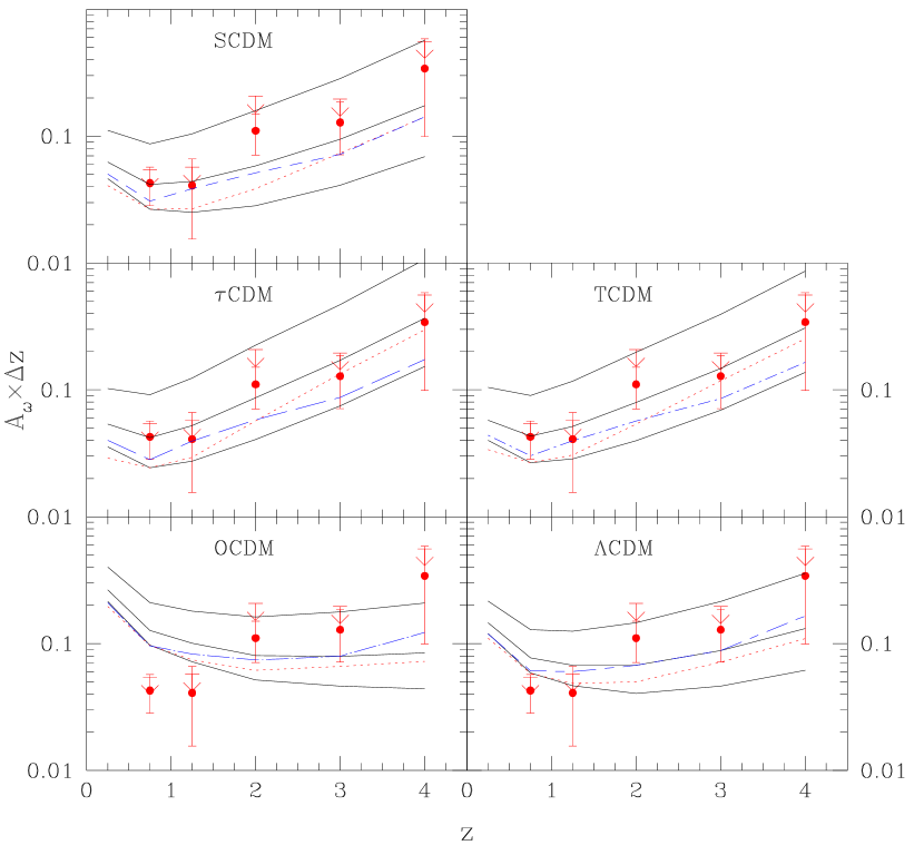
Figure 3: Comparison of the observed $A_{\omega}$ (filled circles for $I_{AB}\leq 28.5$, arrows for the upper limits estimates) with the prediction of the various theoretical models. The solid lines show the measurements expected when a minimum mass $M_{\rm min}=10^{10}$, $10^{11}$ and $10^{12}h^{-1}M_{\odot}$ is assumed; the lower curves refer to smaller masses. The dotted lines show the prediction obtained by using the median masses at any redshift estimated with GISSEL models. The dashed curves correspond to models where the masses necessary to reproduce the observed density of objects in each redshift bin are used.

We have compared our results with the theoretical predictions of a set of different cosmological models belonging to the class of CDM scenario. The halo masses required to match the observations depend on the adopted background cosmology. For Einstein de Sitter (EdS) universes, the SCDM model reproduces the observed measurements if a typical minimum mass of $10^{11}h^{-1}\ M_{\odot}$ is used, while the $\tau$CDM and TCDM models require a lower typical mass of $10^{10}-10^{10.5}h^{-1}\ M_{\odot}$. For OCDM and $\Lambda$CDM models, the mass is a function of redshift, with $M_{\rm min}\leq 10^{10}h^{-1}\ M_{\odot}$ at $z\leq 1$, $10^{11}h^{-1}\ M_{\odot}$ between $1\leq z\leq 3$ and $10^{12}h^{-1}\ M_{\odot}$ at $z\simeq 4$. The higher masses required at high $z$ to reproduce the clustering strength for these models are a consequence of the smaller bias they predict at high redshift compared to the EdS models. At $z\simeq 3$, the clustering strength and the observed density of galaxies are in good agreement with the theoretical predictions for any fashionable cosmological model. At $z\simeq 4$, the present analysis seems to be more discriminant. Due to the remarkably high correlation strength, for some models the observed density of galaxies starts to be inconsistent with the required theoretical halo density. The difference in the predicted masses (a factor $\simeq$ 15 to 30 at $z\simeq$ 3 and 4) between EdS and non-EdS universe models is also highly discriminant and in principle testable in terms of measured velocity dispersions.

A prediction of the hierarchical models is the dependence of the clustering strength on the limiting magnitude of the samples. At $z\simeq 3$ the density of galaxies in the HDF is approximately 65 times higher than the spectroscopic samples of LBGs [1, 12]. Comparing our measurements with the latter a clear trend of decreasing clustering strength with increasing density is detected. This result is in excellent agreement (both qualitatively and quantitatively) with the predictions of hierarchical models [18] and, as noted by Adelberger et al. (1998), suggests the existence of a strong relation between the halo mass and the absolute UV luminosity: more massive haloes host the brighter galaxies.

Finally, we have compared our $\sigma^{\rm gal}_{8}$ to that of the mass predicted for three cosmologies to estimate the bias. For all cases, we found that the bias is an increasing function of redshift with $b(z\simeq 0)\simeq 1$ and $b(z\simeq 4)\simeq 4.5$ (for EdS universes), and $b(z\simeq 0)\simeq 0.5$ and $b(z\simeq 4)\simeq 3$ (for open and $\Lambda$ universes). This result confirms and extends in redshift the results obtained for LBGs at $z\simeq 3$ [1, 12], suggesting that these high-redshift galaxies are located preferentially in the rarer and denser peaks of the underlying matter density field.

What are the descendants of the galaxies observed at $z\simeq 3-4$ in the HDF? In a simple scenario assuming that only one galaxy is hosted by the descendants the resulting local bias implies that the descendants in the case of OCDM and $\Lambda$CDM models can be found among the brightest and more massive galaxies inside clusters, while for EdS universes they are field or normal bright galaxies.

The present results have been obtained in a relatively small field for which the effects of cosmic variance can be important[25]. Nevertheless they show a possibility of challenging cosmological parameters which becomes particularly exciting in view of the rapidly growing wealth of multi-wavelength photometric databases in various deep fields and availability of 10m-class telescopes for spectroscopic follow-up in the optical and near infrared.

3 QSOs Strike Back: Clustering of Absorbers

After all galaxies are exotic objects too, in the sense that they are also biased tracers of mass. There is, however, a way to follow more “normal” matter at high redshifts: the absorption spectra of QSOs, which sensitively probe the gaseous baryonic component of the universe. Sensitivity is the key word: with the present instrumentation it is possible to detect neutral HI column densities down to $10^{12}$ cm^-2, while for example 21 cm radio observations which roughly correspond to the visible extent of a galaxy are limited in the best cases to column densities that are 7 orders of magnitude larger. In this way observations of the Lyman-$\alpha$ forest reveal with an enormous dynamic range very different structures, ranging from fluctuations of the diffuse intergalactic medium to the interstellar medium in protogalactic disks.

In recent times a large database of high-resolution ($\sim 10$ km/s), high-S/N spectra of the Lyman forest has become available, allowing a detailed investigation of the clustering of Lyman-$\alpha$ lines, especially at high redshift, where the density of lines provides particular sensitivity. Cristiani et al (1997) have used more than 1600 Lyman-$\alpha$ ’s to detect a weak but significant signal, with $\xi\simeq 0.2$ on scales of 100 km s^-1 at a $4.6\sigma$ level. Exploring the variations of the clustering as a function of the column density a trend of increasing amplitude of the TPCF with increasing column density is apparent, showing again that bias is at work.

Metal systems show stronger clustering: the CIV CF at $z\simeq 2-2.5$ is consistent with a canonical power-law form with an $r_{o}=3.5$ Mpc and $\gamma\simeq 1.8$ with evidence for an increase of the clustering strength with increasing column density [9, 21]. The relatively large correlation scale indicates that the CIV absorbers are biased tracers of relatively high density regions.

To get a rough idea of the (over- and under-)densities corresponding to Lyman-$\alpha$ absorbers it is useful to estimate their size, on the basis of the statistics of coincidences and anti-coincidences of absorptions in close lines-of-sight to QSO pairs and groups [10], from which one can infer the ionization and the relationship between the observed optical depths and the total density. It turns out that these structures are big (a few hundred kpc), highly ionized and at the lower column densities ($\log N_{HI}\raise-2.0pt\hbox{\hbox to0.0pt{\hbox{$\sim$}\hss}\raise 5.0pt\hbox{$<$}\ }14$) probe weakly biased or even anti-biased regions of the Universe. It makes sense then to compute the power spectrum (PS) of mass density fluctuations and assume that it corresponds to the linear regime. The recovery of the 3-D PS is a complex procedure and various recipes have been proposed by a number of authors [7, 13, 20]. The present results indicate that the PS amplitude is consistent with some scale-invariant, COBE-normalized CDM models (an open model with $\Omega_{0}=0.4$ OCDM, variants of the SCDM) and inconsistent with others (the CCDM model, with $\Omega_{0}=1$, $h=0.5$, $\sigma_{8}=1.2$)[7]. Even with limited dynamic range and substantial statistical uncertainty, a measurement of the PS that has no unknown “bias factors” offers many opportunities for testing theories of structure formation and constraining cosmological parameters.

In a similar fashion, it has been proposed to apply the Alcock-Paczinsky test to QSO groups to investigate the cosmological geometry [13]. This test, based on the comparison between the clustering properties of the (Lyman-$\alpha$) absorbers, namely the TPCF, observed along the line of sight and the corresponding estimate in the transverse direction, is especially sensitive to $\Omega_{\Lambda}$ and should be able to discriminate between an ($\Omega_{m}=0.3,~{}\Lambda=0$) and an ($\Omega_{m}=0.7,~{}\Lambda=0.3$) universe at a $4\sigma$ level by observing $\sim 25$ QSO pairs.

Future prospects look really exciting. Starting at the end of 1999, the echelle spectrograph UVES will be available on UT2 of the VLT, extending, with respect to HIRES at Keck, the possibility of high-resolution ($\Re\sim 50000$) observations down to at least $V\sim 20$ and to a shorter wavelength range (i.e. to more numerous, lower-redshift QSOs). Then (by 2001) the FLAMES facility (see http://http.hq.eso.org/instruments/flames/) will allow observation with UVES of up to 8 QSOs at the same time in a field of 25 arcmin diameter and/or 135 targets in the same area with an intermediate/high resolution spectrograph, GIRAFFE. The Alcock-Paczinsky test and other cosmologically discriminant measures could be carried out in a few nights.

4 Acknowledgments

I wish to thank P.Andreani, S.Arnouts, V.D’Odorico, S.D’Odorico, A.Fontana, E.Giallongo, F. La Franca, F.Lucchin, S.Matarrese, L.Moscardini with whom I have been collaborating and P.Bristow for carefully reading the manuscript.

References

- [1] Adelberger K.L., Steidel C.C., Giavalisco M., Dickinson M.E., Pettini M., Kellogg M., 1998, ApJ 505, 18
- [2] Andreani P., Cristiani S. 1992, ApJ 398, L13
- [3] Arnouts S., Cristiani S., Moscardini L., Matarrese L., Lucchin F., Fontana A., Giallongo E. astro-ph/9902290
- [4] Bagla J.S., 1998, MNRAS 297, 251
- [5] Cavaliere A., Perri M., Vittorini V., 1997, Mem.S.A.It. 68, 27
- [6] Connolly A.J., Szalay A.S., Brunner R.J., 1998, ApJ, 499, L125
- [7] Croft R.A.C., et al., 1998, astro-ph/9809401
- [8] Croom S.M., Shanks T., 1996, MNRAS 281, 89
- [9] D’Odorico V., Cristiani S., D’Odorico S., Fontana A., Giallongo E., 1998a, A&AS 127 217
- [10] D’Odorico V., Cristiani S., D’Odorico S., Fontana A., Giallongo E., Shaver P., 1998b, A&A 339, 678
- [11] Fisher K.B., Bahcall J.N., Kirhakos S., Schneider D. P., 1996, ApJ 468, 469
- [12] Giavalisco M., Steidel C.C., Adelberger K.L., Dickinson M.E., Pettini M., Kellogg M., 1998, ApJ 503, 543
- [13] Hui L., Stebbins A., Burles S., 1999, ApJ 511, L5
- [14] La Franca F., Andreani P., Cristiani S. 1998, ApJ 497, 529
- [15] Magliocchetti M., Maddox S.J., 1998, astro-ph/9811320
- [16] Matarrese S., Coles P., Lucchin F., Moscardini, L., 1997, MNRAS 286, 115
- [17] Mo H.J., Fang L.-Z., 1993, ApJ 410, 493
- [18] Mo H.J., Mao S., White S.D.M., 1999, MNRAS 304, 175
- [19] Moscardini L., Coles P., Lucchin F., Matarrese S., 1998, MNRAS 299, 95
- [20] Nusser A., Haehnelt M., 1999, MNRAS 303, 179
- [21] Quashnock J.M., Vanden Berk D.E., 1998, ApJ 500, 28
- [22] Rengelink R., 1999, Ph.D. Thesis
- [23] Shanks T., Fong R., Boyle B., Peterson B.A., 1987, MNRAS 227, 739
- [24] Shaver P.A., 1984, A&A 136, L9
- [25] Steidel C., 1998, astro-ph/9811400