Foregrounds and Forecasts for the Cosmic Microwave Background

Abstract

One of the main challenges facing upcoming CMB experiments will be to distinguish the cosmological signal from foreground contamination. We present a comprehensive treatment of this problem and study how foregrounds degrade the accuracy with which the Boomerang, MAP and Planck experiments can measure cosmological parameters. Our foreground model includes not only the normalization, frequency dependence and scale dependence for each physical component, but also variations in frequency dependence across the sky. When estimating how accurately cosmological parameters can be measured, we include the important complication that foreground model parameters (we use about 500) must be simultaneously measured from the data as well. Our results are quite encouraging: despite all these complications, precision measurements of most cosmological parameters are degraded by less than a factor of 2 for our main foreground model and by less than a factor of 5 in our most pessimistic scenario. Parameters measured though large-angle polarization signals suffer more degradation: up to 5 in the main model and 25 in the pessimistic case. The foregrounds that are potentially most damaging and therefore most in need of further study are vibrating dust emission and point sources, especially those in the radio frequencies. It is well-known that $E$ and $B$ polarization contain valuable information about reionization and gravity waves, respectively. However, the cross-correlation between polarized and unpolarized foregrounds also deserves further study, as we find that it carries the bulk of the polarization information about most other cosmological parameters.

1. Introduction

Our ability to measure cosmological parameters using the cosmic microwave background (CMB) will only be as good as our understanding of microwave foregrounds, e.g., synchrotron, free-free and dust emission from our own Galaxy and extragalactic objects. For this reason, the recent dramatic progress in the CMB field has stimulated much work on modeling foregrounds and on algorithms for removing them.

Early work on the subject (Lubin & Smoot 1991; Bennett et al. 1992, 1994; Brandt et al. 1994; Dodelson & Stebbins 1994) focused on the frequency dependence of foregrounds and how this could be used to discriminate them from CMB. Work done for the Phase A study of the Planck satellite mission (Tegmark & Efstathiou 1996, hereafter TE96; Bouchet et al. 1996) showed that the scale dependence of foregrounds was also important, often being quite different from the roughly scale-free CMB fluctuations, and that a multifrequency version of Wiener filtering could take advantage of this to improve foreground removal.

The growing interest in CMB polarization, driven by the combination of theoretical utility (Kamionkowski et al. 1997; Zaldarriaga & Seljak 1997; Hu & White 1997) and experimental feasibility (Staggs et al. 1999), has spurred the modeling of foreground polarization signals (e.g., Keating et al. 1998; Zaldarriaga 1998). Such models have been further refined for both the MAP mission (Refregier et al. 1998) and the final Planck science case (AAO 1998), much of which is reviewed in Bouchet & Gispert (1999, hereafter BG99) and de Zotti et al. (1999).

Yet another complication is that the frequency dependence of foregrounds generally varies slightly across the sky. This can be modeled as each foreground having two or more subcomponents (TE96; AAO 1998; BG99) or more generally by introducing the notion of frequency coherence (Tegmark 1998, hereafter T98).

The purpose of the present paper is to assess the impact of foregrounds on CMB experiments, including all of the above-mentioned complications. This is important for two reasons, aside from a general desire to have realistic expectations for future CMB experiments:

1. It helps identify which foregrounds are most damaging and therefore most in need of further study.

2. It is useful for optimizing future missions and for assessing the science impact of design changes to, e.g., Planck.

Such a comprehensive analysis is quite timely, since our knowledge of foregrounds has undergone somewhat of a phase transition during the last year or two: whereas earlier foreground models were quite speculative, generally based on extrapolations from lower or higher frequencies, foregrounds have now been convincingly detected and quantified at CMB frequencies by CMB experiments such as COBE DMR (Kogut et al. 1996, hereafter K96), MAX (Lim et al. 1996), Saskatoon (de Oliveira-Costa et al. 1997), OVRO (Leitch et al. 1997), the 19 GHz survey (de Oliveira-Costa et al. 1998) and Tenerife (de Oliveira-Costa et al. 1999a).

This paper extends prior work in a number of ways. The treatment of spectral variations is more general than in the work for the Planck proposal (TE96; Bersanelli et al. 1996; Bouchet et al. 1999; BG99) and in Knox (1999, hereafter K99). It propagates the effect of foregrounds all the way through to the measurement of cosmological parameters, which has not been previously done except for a limited parameter set (Prunet et al. 1998a). Finally, it quantifies the degradation caused by the need to measure the statistical properties of the foregrounds directly from the CMB data, jointly with the CMB parameters.

The rest of this paper is organized as follows. In §2, we present models for the various physical foreground components. In §3, we present our mathematical formalism for foreground removal. In §4, we apply this to the Boomerang, MAP and Planck missions and compute the level of foreground residuals in the cleaned map for various scenarios. In §5, we compute the extent to which this residual contamination degrades the measurement of cosmological parameters, both when the foreground power spectra are known and when they must be computed from the CMB data itself. In both cases, we study how robust our results are to variations in the foreground model. We summarize our conclusions in §6.

2. Foreground models 1: the physics

The foreground model described in this section is summarized in Table 2. We make three models: one pessimistic (PESS), one middle-of-the-road (MID) and one optimistic (OPT). Since we want to span the entire range of uncertainties, we have made both the PESS and OPT models rather extreme in the (lamentably many) cases where observational constraints are weak or absent. The MID model is intended to be fairly realistic, but somewhat on the conservative (pessimistic) side. A FORTRAN code evaluating these models has been made available at www.sns.ias.edu/$\sim$max/foregrounds.html, and we will continually update this as our foreground knowledge improves.

2.1. Notation

Our foreground model involves specifying the following quantities for each physical component $k$ and each of the four types of polarization power ($P=T$, $E$, $B$ and $X$):

1. Its average frequency dependence $\Theta_{{(k)}}^{P}(\nu)$.

2. Its frequency coherence $\xi_{(k)}^{P}$.

3. Its spatial power spectrum $C_{\ell{(k)}}^{P}$.

Although this notation will be described in great detail in §3, some clarifications are already in order at this point. $\Theta_{{(k)}}^{P}(\nu)$ gives the frequency dependence of the rms fluctuations in thermodynamic temperature referenced to the CMB blackbody. For reference, antenna temperature is converted to thermodynamic temperature by multiplying by

$$c=\left({2\sinh{x\over 2}\over x}\right)^{2},$$ (1)

where $x\equiv h\nu/kT_{\rm cmb}\approx\nu/56.8\,{\rm GHz}$. Specific intensity or surface brightness is converted to antenna temperature by

$$c_{*}\equiv{1\over x^{2}}\>{1\over 2k}\left({hc\over kT_{\rm cmb}}\right)^{2}\approx{1\over x^{2}}\>{10\,{\rm mK}\over{\rm MJy}/{\rm sr}}.$$ (2)

We assume that the frequency dependence is independent of polarization type and angular scale. Note that the latter is not the same as assuming that the frequency dependence of the sky brightness does not vary with position on the sky. The frequency coherence $\xi_{(k)}^{P}$ quantifies this spectral variation as described in §3. For the purpose of this section, it is sufficient to know that $\xi\approx{1/\sqrt{2}\Delta\alpha}$, where $\Delta\alpha$ is the dispersion in the foreground spectral index across the sky. If we write the foreground specific intensity in the form ${I_{\nu}}=f(\nu)\nu^{\alpha}$ for some shape function $f$, then $\Delta\alpha$ is simply the rms fluctuation in $\alpha$. Because our foreground models choose $\Theta$ and $\xi$ to be independent of the polarization type, we will suppress the $P$ superscript in this section. We consider the general case in §5.

We define $C_{\ell}$ in the usual manner, namely as the variance of the amplitude of fluctuations in the $\ell^{\rm th}$ multipole. We then model the power spectra of all components except the CMB anisotropies and the thermal Sunyaev-Zel’dovich (SZ) effect as power laws

$$C_{\ell{(k)}}^{P}=(pA)^{2}\ell^{-\beta},$$ (3)

where $\beta$ and the normalization $pA$ depend on the type of foreground ($k$) and polarization ($P$) as shown in Table 2. For convenience, we factor the normalization into two terms: $A$ gives the normalization of the unpolarized component and $p$ gives the relative normalization of the polarized components. We will explore more general power spectrum models in $\S\ref{JointSec}$.

2.2. What is a foreground and what is a signal?

Figure 1.— The MID model for synchrotron radiation (heavy line). The first three columns show the uncleaned amplitude as a function of scale at 30, 100 and 217 GHz. The rows show the temperature ($T$), cross-correlation ($X$) and $E$-channel polarization, respectively. For reference, the CMB power spectrum of our our fiducial $\Lambda$CDM cosmology (§ 5.1) is also shown (thin solid line) together with the total foreground power including (dotted) and excluding (dashed) Planck detector noise. The second three columns show the foregrounds amplitude when the maps are cleaned according to the optimal procedure in § 4; this method assumes that the foreground properties are well-known. The cleaning depends on the experimental specifications; we show results for Boomerang, MAP and Planck. There is no polarization data in the Boomerang column, since this in an unpolarized experiment.

Of the multitude of physical mechanisms that create microwave fluctuations in the sky, where should the line be drawn between what constitutes a cosmic signal and what is to be considered foreground contamination? All workers in the field agree that effects occurring around or before recombination at $z\sim 10^{3}$ constitute signal, whereas dust, free-free and synchrotron radiation are foregrounds, regardless of whether the origin is in the Milky Way or in extragalactic objects. For the remaining effects, the distinction is less clear and somewhat arbitrary. It has been common to label all effects occurring long after recombination (see Refregier 1999 for a recent review) as foregrounds, which would then include, e.g., the late integrated Sachs-Wolfe (ISW) effect (Sachs & Wolfe 1967; Boughn & Crittenden 1999) and gravitational lensing of the CMB. We will take a different and more goal-oriented approach. When the goal is to measure cosmological parameters, the crucial issue is not when or how the signal was created, but how reliably it can be calculated. We therefore make the following operational definition of what constitutes a foreground:

• A foreground is an effect whose dependence on cosmological parameters we cannot compute accurately from first principles at the present time.

With this definition, gravitational lensing of the CMB, the late ISW effect, and the Ostriker-Vishniac (OV) effect (Ostriker & Vishniac 1986; Vishniac 1987) are not foregrounds, even though the latter is $2^{nd}$ order and non-Gaussian (Hu et al. 1994; Dodelson & Jubas 1995) and the two former jointly create a non-Gaussian bispectrum (Zaldarriaga & Seljak 1999; Goldberg & Spergel 1999). On the other hand, patchy reionization and the thermal SZ effect are foregrounds, since their calculation requires hydrodynamics simulations of reionization (reviewed in Haiman & Knox 1999) and galaxy formation.

2.3. Diffuse galactic foregrounds: synchrotron, free-free & dust emission

Our knowledge of Galactic foregrounds improved substantially during 1998. Whereas older models (e.g., TE96) were mainly based on extrapolations from frequencies far outside the CMB range, a number of statistically significant detections of cross-correlation between new CMB maps and various foreground templates now allow us to normalize many foreground signals directly at the frequencies of interest.

2.3.1 Synchrotron radiation

Figure 2.— Same as Fig. 1, but for free-free emission.

For synchrotron emission in our Galaxy (see Smoot 1999 for a recent review), we model the frequency dependence as $\Theta_{(\rm synch)}(\nu)\propto c(\nu)\nu^{-\alpha}$. Because the spectral index $\alpha$ depends on the energy distribution of relativistic electrons (Rybicki & Lightman 1979), it may vary somewhat across the sky. One also expects a spectral steepening towards higher frequencies, corresponding to a softer electron spectrum (Banday & Wolfendale 1991; Fig 5.3 in Jonas 1999). Based on the data described in Platania et al. (1998), we take $\alpha=2.8$ for our MID estimate for the unpolarized intensity, with a spectral uncertainty $\Delta\alpha=0.15$. As to the power spectrum $\ell^{-\beta}$, the 408 MHz Haslam map suggests $\beta$ of order 2.5 to 3.0 down to its resolution limit $\sim 1^{\circ}$ (TE96, Bouchet et al. 1996), although the interpretation is complicated by striping problems (Finkbeiner et al. 1999). The Parkes survey (Duncan 1997; Duncan 1998, hereafter D98) enables an extension of this down to $4^{\prime}$, i.e., $\ell\sim 900$, and gives $\beta\approx 2.4$ (de Oliveira-Costa et al. 1999b) – we adopt this value to be conservative, since we will normalize on large angular scales. This agrees qualitatively with theoretical power spectrum estimates assuming isotropic turbulence with a $k^{-11/3}$ Kolmogorov spectrum for the Galactic magnetic field (Tchepurnov 1997).

For the polarized synchrotron component, our observational knowledge is unfortunately very incomplete. The only available measurement of the polarized synchrotron power spectrum is from the 2.4 GHz D98 maps, which exhibit a much bluer power spectrum in polarization than in intensity, with $\beta\sim 1.0$ instead of $2.5$ (de Oliveira-Costa et al. 1999b). However, at least part of this patchiness is due to modulations in Faraday rotation by small-scale variations in the Galactic magnetic field. These results therefore cannot be readily extrapolated to higher frequencies such as 50 GHz, where Faraday rotation (which scales as $\nu^{-2}$) becomes irrelevant. A second difficulty lies in extrapolating from the D98 observing region around the Galactic plane to higher latitudes, where the smaller mean distance to visible emission sources may well result in less small-scale power in the angular distribution. The polarization maps of Brouw & Spoelstra (1976) extend to high Galactic latitudes and up to 1.4 GHz but unfortunately are undersampled, making it difficult to draw inferences about the polarized power spectrum from them. To bracket the uncertainty, we take $\beta=1.0$ for PESS, $\beta=1.4$ for MID and $\beta=3$ (the same power spectrum slope as for the unpolarized intensity) for OPT.

Although Faraday rotation softens the frequency dependence to $\alpha\sim 1.6$ for $\nu\mathrel{\hbox to0.0pt{\lower 3.0pt\hbox{$\mathchar 536\relax$}\hss}\raise 2.0pt\hbox{$\mathchar 316\relax$}}5\>{\rm GHz}$ (de Oliveira-Costa et al. 1999b), we assume that the polarization fraction saturates to a constant value for $\nu\gg 10\>{\rm GHz}$, as Faraday rotation becomes irrelevant. We therefore use the same $\alpha$ and $\Delta\alpha$ for polarized and unpolarized synchrotron radiation.

For the MID scenario, we normalize the unpolarized synchrotron component to the cross-correlation with the 19 GHz map found by de Oliveira-Costa et al. (1998). This gives $\sigma=52\pm 17{\rm\mu K}$ on the $3^{\circ}$ scale for a $20^{\circ}$ galactic cut, retaining roughly the cleanest 65% of the sky. This agrees well with the synchrotron amplitude obtained in the cross-correlation analyses using the Tenerife 10 and 15 GHz maps (de Oliveira-Costa et al. 1999a; Jones 1999). For the PESS model, we use the $7.1{\rm\mu K}$ upper limit from COBE DMR found by K96) at 31.5 GHz on the $7^{\circ}$ scale.

The degree of synchrotron polarization typically varies between 10% and 75% on large scales (Brouw & Spoelstra 1976), so we normalize our models to give 10% (OPT), 30% (MID) and 75% (PESS) rms polarization on COBE scales. Because the polarization power spectra in the MID and PESS models are blue-tilted relative to the intensity power spectra, the rms polarization exceeds 100% in these models on sub-degree scales. This is physically possible because the $\ell=0$ contribution to the intensity map has been ignored; in an extreme case, it is possible to have polarization fluctuations even with a perfectly smooth intensity map.

2.3.2 Free-free emission

Figure 3.— Same as Fig. 1, but for thermal (vibrational) dust emission.

Of all diffuse Galactic foregrounds, free-free emission is the one whose frequency dependence is best known. We model it as a power law $\Theta_{\rm(ff)}(\nu)\propto c(\nu)\nu^{-\alpha}$, where $\alpha=2.15$ and $\Delta\alpha=0.02$. In our OPT and MID scenarios, we assume that this emission is completely unpolarized (Rybicki & Lightman 1979). However, free-free emission can become polarized by Thomson scattering off of free electrons within the H_II region itself (Keating et al. 1998; Davies & Wilkinson 1999). We therefore assume a 10% polarization level in the PESS model, which corresponds to the most extreme case of an optically thick cloud and no line-of-sight superpositions of interloper H_II-regions.

Although the spectrum of free-free emission is well-known, the amplitude and power spectrum are not. Since dust dominates at high frequencies, synchrotron at low frequencies and CMB in the intermediate range, it is difficult to obtain a spatial template of free-free emission. H$\alpha$ maps should be able to play this role shortly (see McCullough et al. 1999 for a review), but in the interim, we must make do with more indirect estimates. K96 obtained a 2-sigma upper limit of $14.2\>{\rm\mu K}$ for the rms free-free fluctuations at 53 GHz by taking a linear combination of the three COBE DMR maps that projected out the CMB—we use this normalization for our PESS model, and it is consistent with the upper limit of Coble et al. (1999). K96 also found a highly significant detection of a component correlated with the DIRBE dust maps whose frequency dependence was consistent with $\alpha=2.15$. Similar correlations have been detected for the Saskatoon data (de Oliveira-Costa et al. 1997), the 19 GHz map (de Oliveira-Costa et al. 1998) and the OVRO Ring experiment (Leitch et al. 1997)—see Kogut (1999) for a review of this puzzle. For our MID model, we will follow K96 in assuming that this component is in fact free-free emission, which gives an rms of $7.6\>{\rm\mu K}$ at 53 GHz on DMR scales for a $30^{\circ}$ galaxy cut. For the power spectrum shape, we assume $\beta=3$ for OPT and MID (as for dust) and $\beta=2.2$ (as for synchrotron radiation) for PESS. Again this agrees qualitatively with theoretical estimates assuming a isotropic turbulence with a Kolmogorov spectrum for electron density fluctuations in the interstellar medium (Tchepurnov 1997).

2.3.3 Dust

Figure 4.— Same as Fig. 1, but for thermal spinning dust emission.

For vibrational emission from dust grains in the interstellar medium, we model the frequency dependence as

$$\Theta_{\rm(dust)}(\nu)\propto c(\nu)c_{*}(\nu){\nu^{3+\alpha}\over e^{h\nu/kT_{\rm(dust)}}-1}.$$ (5)

We assume a dust temperature $T_{\rm(dust)}=18{\rm K}$ (MID) and an emissivity $\alpha=1.7$ (K96). The effective emissivity could vary across the sky if the relative proportions of different types of dust grains shift, and modulations in the dust temperature with, e.g., galactic latitude, would further increase the dispersion in the frequency dependence. Estimates of $\alpha$ have ranged between 1.4 and 2.0 across the sky and in multi-component models (e.g., Reach et al. 1995). Although recent work has weakened the evidence for multiple dust temperatures, at least in the cleanest parts of the sky (see the discussion in BG99), joint analysis of the DIRBE and FIRAS data sets has given strong indications that two components with different emissivities are present even at high Galactic latitudes (Schlegel et al. 1998; Finkbeiner & Schlegel 1999). We therefore we take $\Delta\alpha=0.3$ (MID).

As to the power spectrum $\ell^{-\beta}$, the combined DIRBE and IRAS dust maps suggest a slightly shallower slope $\beta=2.5$ (Schlegel et al. 1998) than earlier work finding $\beta\approx 3.0$ (Gautier et al. 1992; Low & Cutri 1994; Guarini et al. 1995; TE96). However, a recent analysis of the DIRBE maps has shown no evidence of a departure from an $\ell^{-3}$ power law for $\ell\mathrel{\hbox to0.0pt{\lower 3.0pt\hbox{$\mathchar 536\relax$}\hss}\raise 2.0pt\hbox{$\mathchar 316\relax$}}300$ (Wright 1998); we will use this value for the MID model because only the behavior at low $\ell$ is important for the present analysis.

Dust emission may be highly polarized if the grains align in the local magnetic field (Wright 1987). For the polarization power spectra, we use the models of Prunet et al. (1998b) and Prunet & Lazarian (1999), which give $\beta=1.3$ for $E$, $\beta=1.4$ for $B$, and $\beta=1.95$ for $X$. This corresponds to about 1% polarization in $E$ on the $7^{\circ}$ scale and greater polarization on smaller scales.

We normalize the (MID) unpolarized dust power spectrum using the DIRBE-DMR cross-correlation analysis of K96, which gives rms fluctuations of $2.9{\rm\mu K}$ at 53 GHz on the COBE angular scale. This is is a factor 2.3 higher than the Prunet et al. model at 100 GHz, and we boost their polarization normalization by the same factor to be conservative. The OPT and PESS normalizations are a factor of 3 lower and higher, respectively, for $T$ on the $7^{\circ}$ scale. The $E$ and $B$ normalization is a factor of three lower for OPT but a factor 10 higher for PESS, the latter corresponding to about 15% polarization on the 5’ scale.

2.3.4 “Anomalous” dust emission

Figure 5.— Same as Fig. 1, but for the thermal SZ effect from filaments.

An alternative interpretation of the dust-correlated foreground component described in §2.3.2 has been proposed by Draine & Lazarian (1998, hereafter DL98). They identify it as dust emission after all but radiating via rotational rather than vibrational excitations. The latest Tenerife measurements strongly support this idea (de Oliveira-Costa et al. 1999) since the observed turnover in the spectrum with a decrease from 15 to 10 GHz is incompatible with free-free emission alone. This emission will be dominated by the very smallest dust grains (more appropriately called clusters, since they may consist of only $\sim 10^{2}$ atoms). Many DL98 models are well fit by spectra of the form of equation (5), but with rather unusual parameters. For our MID model, we take the rather typical DL98 model that is fit by $T_{\rm(dust)}=0.25{\rm K}$, $\alpha=2.4$. However, the range of theoretically and observationally allowed spectra is very large, and magnetic-dipole dust emission could have yet another spectral signature (Draine & Lazarian 1999). We adopt a very large spectral uncertainty $\Delta\alpha=0.5$ to reflect this. For our pessimistic model, we adopt an extremely blue ($\beta=1.2$) power spectrum for this component, since the work of Leitch et al. (1997) indicates that this component may be very inhomogeneous on small scales.

We normalize our MID model so that spinning dust accounts for the entire dust-correlated signal at 31.5 GHz. This double-counting is of course mildly conservative, since we normalized free-free emission in the same way. Given the complete absence of power spectrum measurements for this component, the MID model simply assumes the same power spectra as for regular dust emission, both in intensity and polarization, as well as the same polarization fractions. The PESS scenario gives 10% polarization (Prunet & Lazarian 1999). In the OPT scenario, we assume no spinning dust component at all.

Throughout this paper, we are assuming that the different foreground components are uncorrelated. This is probably not the case for, e.g., spinning and vibrating dust. Once these correlations are better measured, one can take advantage of this information to improve the foreground removal, as well as define linear combinations of the foregrounds that are uncorrelated.

2.4. Thermal and kinematic SZ effect

The thermal SZ effect (Sunyaev & Zel’dovich 1970) is the characteristic distortion of the CMB spectrum caused by hot ionized gas in galaxy clusters and filaments, whereas the kinematic SZ effect is the temperature fluctuation occurring when motion of such gas Doppler shifts the CMB spectrum. The dominant part of the kinematic SZ effect caused by matter fluctuations in the linear regime is known as the Ostriker-Vishniac (OV) effect (Vishniac 1987), and can be accurately computed using perturbation theory (Hu & White 1996). According to the definition we gave in §2, a process is a foreground only if it cannot be accurately computed at the present time, so only part of the kinetic SZ effect qualifies as a foreground: the small correction to the OV effect caused by nonlinear structures, whose computations would require accurate hydrodynamics simulations. Since this correction is likely to be small, we will not attempt to model it in the present paper.

The thermal SZ effect, on the other hand, does qualify as a foreground (Holder & Carlstrom 1999). Just as we assumed removal of bright radio and IR point sources, we will assume that cores of known clusters have been discarded from the CMB maps. In addition to removing known clusters, it has been estimated that of order $10^{4}$ additional clusters can be detected (and removed) using the Planck data (de Luca et al. 1995; Aghanim et al. 1997; Refregier et al. 1998; Refregier 1999), reducing both the kinematic and thermal SZ effect from clusters to negligible levels. The SZ foreground will therefore be dominated by the thermal effect from filaments and other large-scale structures outside of clusters. As our MID estimate of this effect, we use the semianalytic results of Persi et al. (1995), whose $\Lambda$CDM model is well fit by the broken power law power spectrum

$$\ell^{2}C_{\ell\rm(SZ)}=(0.26{\rm\mu K}\>A)^{2}\left[\ell^{n_{1}\gamma}+\left({\ell\over\ell_{*}}\right)^{n_{2}\gamma}\right]^{1/\gamma},$$ (6)

Here $n_{1}=1$ and $n_{2}=-2$ are the asymptotic slopes at low and high $\ell$ respectively, while $\gamma=-0.25$ gives the sharpness of the peak, which is located at $\ell_{peak}=4000$ using $\ell_{*}\equiv(-n_{1}/n_{2})^{-1/\gamma n_{2}}\ell_{peak}^{1-n_{1}/n_{2}}$. Equation (6) is normalized in the Rayleigh-Jeans limit $\nu\ll$ 56 GHz for $A=1$. Our PESS model is normalized an order of magnitude higher, roughly in line with current observational upper limits. Relativistic corrections to the frequency dependence are important for hot clusters (Wright 1979; Rephaeli 1995; Stebbins 1997). Since we are throwing out the known clusters and the filaments that dominate the remaining effect are much cooler, the nonrelativistic SZ-spectrum should be quite a good approximation. In thermodynamic temperature, this is given by (Sunyaev & Zel’dovich 1970)

$$\Theta_{\rm(SZ)}(\nu)\propto 2-{x\over 2}\coth{x\over 2}\to 1\quad\hbox{as}\quad x\to 0,$$ (7)

where $x\equiv h\nu/kT_{\rm cmb}\approx\nu/56.8\,{\rm GHz}$.

2.5. Detector noise

Table 1

CMB Experimental Specifications Experiment $\nu$ FWHM $10^{6}\Delta T/T$ $10^{6}\Delta T/T$ (unpol) (pol) Boomerang 90 20 7.4  $\cdots$ 150 12 5.7  $\cdots$ 240 12 10  $\cdots$ 400 12 80  $\cdots$ MAP 22 56 4.1 5.9 30 41 5.7 8.0 40 28 8.2 11.6 60 21 11.0 15.6 90 13 18.3 25.9 Planck 30 33 1.6 2.3 44 23 2.4 3.4 70 14 3.6 5.1 100 10 4.3 6.1 100 10.7 1.7  $\cdots$ 143 8.0 2.0 3.7 217 5.5 4.3 8.9 353 5.0 14.4  $\cdots$ 545 5.0 147 208 857 5.0 6670  $\cdots$

NOTES.—Specifications used for Boomerang, MAP and Planck. Frequencies $\nu$ are in GHz. Full width at half maxima (FWHM) of the beams are in arcminutes. Boomerang covers a fraction $f_{\rm sky}\approx 2.6\%$ of the sky, while we assume a useful sky fraction of 65% for MAP and Planck. $(w^{P})^{-1/2}=\Delta T\times{\rm FWHM}\times\pi/10800$. In practice, we combine the two Planck 100 GHz channels into one channel with FWHM of 10’.7 and $\Delta T/T$ of 1.57 and $5.68\times 10^{-6}$ for unpolarized and polarized channels, respectively.

As first pointed out by Knox (1995), detector noise can be conveniently treated as an additional sky signal with power spectrum

$$C_{\ell\rm(noise)}^{P}=(w^{P})^{-1}e^{\theta^{2}\ell(\ell+1)}$$ (8)

if the experimental beam is Gaussian with width $\theta$ in radians (the full-width-half-maximum is given by FWHM$=\sqrt{8\ln 2}\>\theta$). Here the sensitivity measure $1/w^{P}$ is defined as the noise variance per pixel times the pixel area in steradians for $P=T,E,B$. As shown in Appendix A of Tegmark (1997b), equation (8) remains valid even for incomplete sky coverage — the corresponding information loss causes correlations between the different noise multipoles, but not an increase in their variance. The noise variance $(\Delta T/T)^{2}$ per pixel of area FWHM² is given in Table 1. We assume that that this pixel noise is equal and uncorrelated for the two measured Stokes parameters $Q$ and $U$, which means that the same noise value applies to $E$ and $B$ ($w^{E}=w^{B}$). We also assume that the noise is uncorrelated between intensity and polarization, so that $1/w^{X}=0$. For an experiment like MAP where intensity/polarization is measured by adding/subtracting pairs of linearly polarized receivers, $w^{E}=w^{B}=w^{T}/2$ (one pair measures $Q$ and $T$, another does $U$ and $T$, and all four measurements are independent with identical variance).

2.6. Point sources

Figure 6.— Same as Fig. 1, but for radio and far infrared point sources.

The TE96 point-source model assumed that all sources above some flux cut $S_{c}$ could be removed from the map (by discarding the contaminated pixels, say) and gave the power spectrum due to Poisson fluctuations in the unresolved remainder. Here we will make the conservative assumption that no external source templates will be available at these frequencies, so that point sources must be detected internally from the CMB maps themselves, say as $5-\sigma$ outlyers. Especially for high sensitivity experiments such as Planck, the main sources of confusion noise are the CMB fluctuations themselves (and dust at very high frequencies). It is therefore desirable to spatially band-pass filter the maps to suppress CMB and detector noise fluctuations before performing the point-source search. Tegmark & de Oliveira-Costa (1998) derive such a procedure and find that the resulting minimal rms confusion noise $\sigma$ for point-source detection (in MJy) is given by

$$\sigma(\nu)=[c(\nu)c_{*}(\nu)]^{-1}\left[\sum_{\ell}\left({2\ell+1\over 4\pi}\right)/C_{\ell\rm(tot)}(\nu)\right]^{-1/2},$$ (9)

where $C_{\ell\rm(tot)}$ is the sum of the power spectra of other foregrounds, noise and CMB. Tegmark & de Oliveira-Costa (1998) find that this filtering lowers the point-source detection threshold $\sigma$ by a factor between 2.5 and 18 for Planck. Refregier et al. (1998) present such an analysis for the MAP satellite.

Once the flux cut $S_{c}=5\sigma$ has been computed using our foreground and CMB model (the latter is described in §5), we calculate the point-source power spectrum using the expression (TE96)

$$C_{\ell\rm(ps)}^{T}(\nu) \equiv \left[\Theta_{(\rm ps)}(\nu)\right]^{2}C_{\ell(\rm ps)}^{T}$$ (10)

$$= [c(\nu)c_{*}(\nu)]^{2}\int_{0}^{S_{c}}\left[-{\partial n\over\partial S}\right](S,\nu)S^{2}dS.$$

Here $n(S,\nu)$ gives the source counts, i.e., the number of point sources per steradian whose flux exceeds $S$ at the frequency $\nu$. We evaluate this integral, which is independent of $\ell$, separately for each frequency channel using the source count model of Toffolatti et al. (1998, 1999; see also Guiderdoni et al. 1998, Guiderdoni 1999). We then multiply the resulting power spectrum by the normalization fudge factors $(pA)^{2}$ given in Table 2. These source count models are consistent with the upper limits from the SCUBA experiment (Scott & White 1999; Mann et al. 1999) and other observations (Gawiser et al. 1998). As stressed by, e.g., Franceschini et al. (1989), point-source clustering can create additional large-scale power. However, calculations of this effect (TE96; Toffolatti et al. 1998; Cress et al. 1996) suggest that it is diluted by angular projection down to levels that are negligible compared with the Poisson term of equation (10) (c.f., Scott & White 1999). The same holds for the effect of weak lensing modulation the flux cut (Tegmark & Villumsen 1997).

This treatment is rather conservative in that it makes no assumptions about our ability to model the frequency dependence of point sources. In other words, it assumes that one can remove a source from a map only if one actually detects it at that particular frequency. In practice, one might opt to discard pixels as contaminated if they contain a detected point source at other nearby frequencies as well, further reducing the residual $\sigma_{\rm ps}$. Since most point sources have a spectrum substantially different from CMB, the detection threshold can also be pushed below that of equation (9) by taking linear combinations of band-pass filtered versions of different channels, tailored to subtract out say the CMB and/or dust signals.

The frequency dependence of the residual point sources has a distinctly bimodal distribution, corresponding to radio sources (blazars, etc.) and far infrared sources (early dusty galaxies, etc.). Since these are modeled separately in Toffolatti et al. (1998), we treat them as two independent components, greatly reducing the effective spectral index uncertainty. We take $\Delta\alpha=0.5$ for the radio sources in the MID model. If measurements at different frequencies are not taken simultaneously, time-variability of the sources will increase this number (Gutierrez et al. 1999). A more detailed model of the frequency coherence of IR point sources is given by in Fig E.5 in the HFI report (AAO 1998), reprinted as Fig. 5b in BG99), suggesting that $\Delta\alpha$ may be smaller for this population. We therefore assume $\Delta\alpha=0.3$ for the IR point sources (MID).

For the polarization power spectra, we conservatively assume that the radio sources are 10% polarized and the IR sources are 5% polarized. Point sources are one of the few foregrounds whose polarization is not likely to be important. This is because the amplitude relative to noise is always lower in polarization: detector noise is typically “141% polarized” in the sense that it is at least as high in the polarization maps as in the intensity maps, usually by a factor $\sqrt{2}$.

Figure 7.— This figure summarizes the frequency and scale dependence of our foreground models for the optimistic (OPT), middle-of-the-road (MID) and pessimistic (PESS) scenarios described in the text. The colored regions show the parts of parameter space where the foreground fluctuations exceed a level $\delta T_{*}$ characteristic of the CMB, and correspond to synchrotron (magenta), free-free (cyan) and vibrational dust emission (red), rotational dust emission (blue) and the thermal SZ effect (yellow). For point sources, the residual is experiment-specific since it depends on the flux cut down to which point sources can be detected and excised—it is shown separately for MAP and Planck as thick green lines. The black boxes show where detector noise is less than $\delta T_{*}$ for MAP and Planck. The thresholds in $Q_{flat}\equiv(5/12)^{1/2}\delta T_{*}$ are $20{\rm\mu K}$, $3{\rm\mu K}$ and $0.5{\rm\mu K}$ for unpolarized, cross-polarized and $E$-polarized fluctuations, respectively. The $B$-spectra are similar to those shown for $E$-polarization.

Figure 8.— The frequency dependence of our unpolarized foregrounds is shown for three angular scales ($\ell=2$, $\ell=200$ and $\ell=2000$) for the optimistic (OPT), middle-of-the-road (MID) and pessimistic (PESS) scenarios described in the text. The thin curves correspond to synchrotron radiation (short-dashed), free-free emission (long-dashed), spinning dust (solid), vibrational dust (dotted), point sources (dot-dashed) and SZ (solid grey/yellow). The thick curves show the CMB (horizontal line) and the total for all foregrounds.

Table 2

Foreground Model Parameters OPTIMISTIC MIDDLE-OF-ROAD PESSIMISTIC $\alpha$ $\Delta\alpha$ $\beta$ $p$ $\alpha$ $\Delta\alpha$ $\beta$ $p$ $\alpha$ $\Delta\alpha$ $\beta$ $p$ Free-free T 2.15 .01 3 1 2.15 .02 3 1 2.10 .04 2.2 1 emission E  $\cdots$  $\cdots$  $\cdots$ 0  $\cdots$  $\cdots$  $\cdots$ 0 2.10 .04 2.2 0.1 B  $\cdots$  $\cdots$  $\cdots$ 0  $\cdots$  $\cdots$  $\cdots$ 0 2.10 .04 2.2 0.1 X  $\cdots$  $\cdots$  $\cdots$ 0  $\cdots$  $\cdots$  $\cdots$ 0 2.10 .04 2.2 0.3 $\nu_{*}=31.5$ GHz $A=30{\rm\mu K}$ $A=70{\rm\mu K}$ $A=77{\rm\mu K}$ Synchrotron T 2.9 .1 3 1 2.8 .15 2.4 1 2.6 .3 2.2 1 radiation E 2.9 .1 3 .1 2.8 .15 1.4 .13 2.6 .3 1.0 .25 B 2.9 .1 3 .1 2.8 .15 1.4 .13 2.6 .3 1.0 .25 X 2.9 .1 3 .2 2.8 .15 1.9 .3 2.6 .3 1.6 .4 $\nu_{*}=19$ GHz $A=50{\rm\mu K}$ $A=101{\rm\mu K}$ $A=192{\rm\mu K}$ Vibrating T 2.0 .1 3 1 1.7 .3 3 1 1.4 .5 2.5 1 dust E 2.0 .1 3 .01 1.7 .3 1.3 .0022 1.4 .5 1.2 .011 B 2.0 .1 3 .01 1.7 .3 1.4 .0024 1.4 .5 1.2 .011 X 2.0 .1 3 0.03 1.7 .3 1.95 .0098 1.4 .5 1.85 .02 $\nu_{*}=90$ GHz $T=20$K, $A=9.5{\rm\mu K}$ $T=18$K, $A=24{\rm\mu K}$ $T=16$K, $A=45{\rm\mu K}$ Rotating T  $\cdots$  $\cdots$  $\cdots$ 0 2.4 .5 3 1 2.4 1 1.2 1 dust E  $\cdots$  $\cdots$  $\cdots$ 0 2.4 .5 1.3 .0022 2.4 1 1.2 .1 B  $\cdots$  $\cdots$  $\cdots$ 0 2.4 .5 1.4 .0024 2.4 1 1.2 .1 X  $\cdots$  $\cdots$  $\cdots$ 0 2.4 .5 1.95 .0098 2.4 1 1.2 .2 $\nu_{*}=31.5$ GHz $T=0.25$K, $A=70{\rm\mu K}$ $T=0.25$K, $A=32{\rm\mu K}$ Thermal T text .01 text 1 text .02 text 1 text .05 text 1 SZ E  $\cdots$  $\cdots$  $\cdots$ 0  $\cdots$  $\cdots$  $\cdots$ 0  $\cdots$  $\cdots$  $\cdots$ 0 B  $\cdots$  $\cdots$  $\cdots$ 0  $\cdots$  $\cdots$  $\cdots$ 0  $\cdots$  $\cdots$  $\cdots$ 0 X  $\cdots$  $\cdots$  $\cdots$ 0  $\cdots$  $\cdots$  $\cdots$ 0  $\cdots$  $\cdots$  $\cdots$ 0 $\nu_{*}=10$ GHz eq. (6), (7), $A=.3$ eq. (6), (7), $A=1$ eq. (6), (7), $A=10$ Radio T text .3 0 1 text .5 0 1 text 1 0 1 point E text .3 0 .05 text .5 0 .1 text 1 0 .2 sources B text .3 0 .05 text .5 0 .1 text 1 0 .2 X text .3 0 .1 text .5 0 .2 text 1 0 .3 eq. (10), $A=.3$ eq. (10), $A=1$ eq. (10), $A=5$ IR T text .1 0 1 text .3 0 1 text .5 0 1 point E text  $\cdots$ 0 0 text .3 0 .05 text .5 0 .1 sources B text  $\cdots$ 0 0 text .3 0 .05 text .5 0 .1 X text  $\cdots$ 0 0 text .3 0 .1 text .5 0 .2 eq. (10), $A=.3$ eq. (10), $A=1$ eq. (10), $A=5$

NOTES.—Our optimistic (OPT), middle-of-the-road (MID) and pessimistic (PESS) foreground models. The frequency dependence is normalized so that $\Theta(\nu_{*})=1$. The power spectrum normalization is given by $(pA)^{2}$, as specified by equation (3) (for free-free, synchrotron and dust emission), equation (6) (for the thermal SZ effect) and equation (10) (for point sources). To avoid a profusion of large numbers in the table, we have factored the total normalization amplitude $pA$ into an overall constant $A$ and a small dimensionless correction factor $p$ that can be interpret polarization percentage (unless the polarized and unpolarized power spectra have different slopes). The label “text” indicates that the parameterization is to be found in the text using the given equations.

We conclude this section with some estimates of when point sources are important. As shown in Tegmark & Villumsen (1997), the rms fluctuation (in $\mu$K) due to residual point sources is

$$\sigma_{\rm ps}\approx\sqrt{\gamma-1\over 3-\gamma}N^{1/2}5\sigma_{\rm conf},$$ (11)

where $N\equiv\pi\theta^{2}n(S_{c})$ is the number of sources removed per beam area, $\sigma_{\rm conf}\equiv\sigma cc_{*}/2\pi\theta^{2}$ is the confusion noise of equation (9) converted from Jy into ${\rm\mu K}$, and the source counts have been approximated by a power law $n^{\prime}(S)\propto S^{-\gamma}$ near the flux cut. Since relevant values for $\gamma$ are typically in the range 1.5–2.5 (see references in Tegmark & Villumsen 1997), the first term is of order unity. The best attainable $\sigma_{\rm conf}$ is typically 3-5 times $\sigma_{\rm n}$, the rms detector noise per pixel (Tegmark & de Oliveira-Costa 1998). Point sources have only a minor impact on a CMB experiment if $\sigma_{\rm ps}\ll\sigma_{\rm n}$ because their power spectra have the same shape as that for detector noise (apart from the noise increase below the beam scale). Equation (11) therefore tells us that using the CMB map itself for point-source removal is quite adequate as long as $N\ll(4\times 5)^{-2}=0.002$. Conversely, if there are more sources per beam than this rule of thumb indicates, then an external point-source template will be needed to reduce the point-source contribution to a subdominant level.

2.7. Foreground model summary

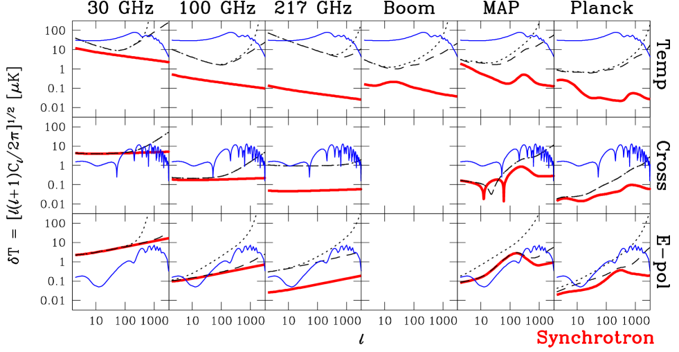
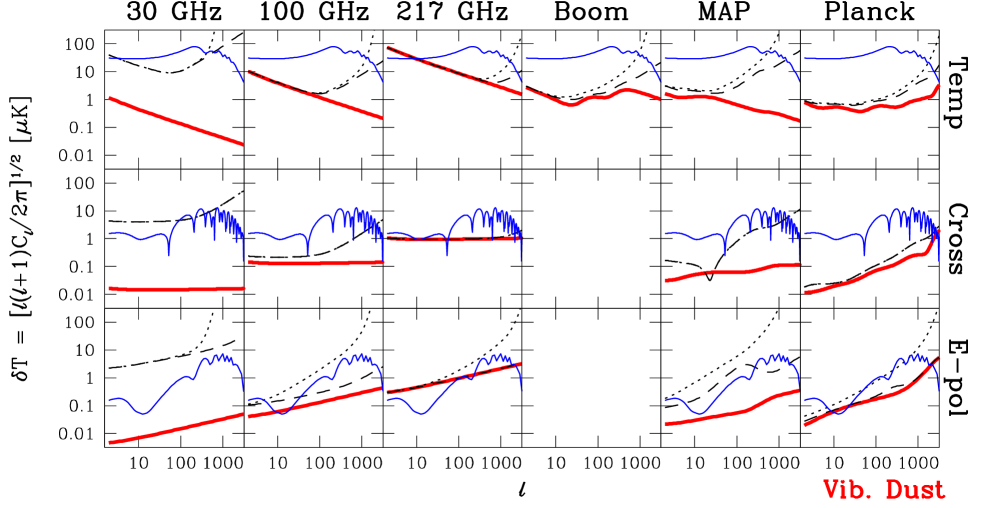
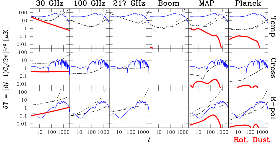
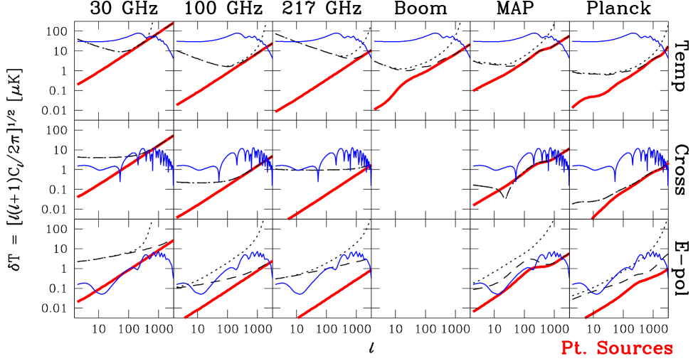
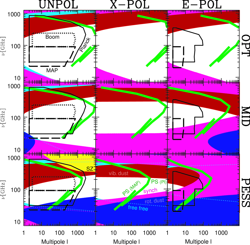
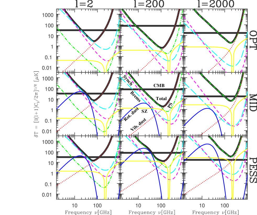
The specifications of our foreground models are given in Table 2. The power spectrum and frequency dependence is summarized in Figure 7, which follows TE96 in showing where the various foregrounds dominate over a typical CMB signal. More details about each foreground are given in figures 1–6, which show the power spectra at three characteristic frequencies. Figure 8 shows the frequency dependence of the foregrounds on three different angular scales.

3. Foreground models 2: the math

3.1. Notation

As described in T98 and further elaborated by White (1998), foregrounds can be treated as simply an additional source of noise that is correlated between frequency channels. This leads to a natural way of parameterizing them as well as to a useful way of removing them. Let us first express this in its most general mathematical form, and then specialize to a case appropriate for our present application of accuracy forecasting.

Consider a pixelized CMB sky map (the “true sky”) at some angular resolution $\theta_{0}$ consisting of $M$ numbers $x_{1},...,x_{M}$, where $x_{i}$ is the temperature in the $i^{th}$ pixel. Suppose that we have single-frequency data sets at our disposal at $F$ different frequencies $\nu_{f}$ ($f=1,2,...,F$) consisting of $N_{f}$ numbers $y^{f}_{1}$, $y^{f}_{2},...,y^{f}_{N_{f}}$, each probing some linear combination of the sky temperatures $x_{i}$. Grouping these numbers into vectors ${\bf x}$, ${\bf y}^{1}$, ${\bf y}^{2},...,{\bf y}^{F}$ of length $M$, $N_{1}$, $N_{2},...,N_{F}$ (these lengths are all generally all different), we can generally write

$${\bf y}^{f}={\bf A}^{f}{\bf x}+{\bf n}^{f}$$ (12)

for some known $N_{f}\times M$ scan strategy matrices ${\bf A}^{f}$ incorporating the beam shapes and some random vectors ${\bf n}^{f}$ incorporating instrumental noise and foreground contamination. The special case where the $F$ data sets are simply sky maps with resolution $\theta_{0}$ corresponds to ${\bf A}^{f}={\bf I}$. If the data sets are maps with different angular resolutions $\theta_{f}\geq\theta_{0}$, then

$${\bf A}^{f}_{ij}={1\over 2\pi(\Delta\theta_{f})^{2}}e^{-{1\over 2}{\left(\theta_{ij}\over\Delta\theta_{f}\right)^{2}}}$$ (13)

if the beams are Gaussian, where $\theta_{ij}=\cos^{-1}(\widehat{{\bf r}}_{i}\cdot\widehat{{\bf r}}_{j})$ is the angular separation between pixels in directions $\widehat{{\bf r}}_{i}$ and $\widehat{{\bf r}}_{j}$ and $\Delta\theta_{f}=(\theta_{f}^{2}-\theta_{0}^{2})^{1/2}$ is the extra smoothing in map $f$. Equation (12) is completely general, however, since the scan strategy matrix ${\bf A}^{f}$ can also incorporate complications such as elliptical and non-Gaussian beams, triple beams, interferometer beams, or oblong synthesized beams (e.g. Saskatoon). Of course, the data sets need not be different channels observed by the same experiment—for instance, one might wish to use the 408 MHz Haslam survey as an additional “channel”.

It is useful to define the larger $(\sum_{f}N_{f})\times M$ matrix and the $(\sum_{f}N_{f})$-dimensional vectors

$${\bf A}\equiv\left(\hskip-5.69046pt\begin{tabular}[]{c}${\bf A}^{1}$\\ $\vdots$\\ ${\bf A}^{F}$\end{tabular}\hskip-5.69046pt\right),\quad{\bf y}\equiv\left(\hskip-5.69046pt\begin{tabular}[]{c}${\bf y}^{1}$\\ $\vdots$\\ ${\bf y}^{F}$\end{tabular}\hskip-5.69046pt\right),\quad{\bf n}\equiv\left(\hskip-5.69046pt\begin{tabular}[]{c}${\bf n}^{1}$\\ $\vdots$\\ ${\bf n}^{F}$\end{tabular}\hskip-5.69046pt\right).\quad$$ (14)

This allows us to rewrite equation (12) as

$${\bf y}={\bf A}{\bf x}+{\bf n},$$ (15)

a set of linear equations that would be highly over-determined if it were not for the presence of unknown noise $n$.

It is straightforward to include polarization information in our formalism. In this case, we wish to measure not one sky map but three: the unpolarized temperature map ${\bf x}^{T}$ and the “electric” and “magnetic” polarization maps ${\bf x}^{E}$ and ${\bf x}^{B}$ (Kamionkowski et al. 1997; Zaldarriaga & Seljak 1997). The latter are linearly related to the Stokes Q and U maps and have the advantage of being independent of the choice of coordinate system and more directly linked to the physical processes that make the CMB polarized. Grouping them into a single vector

$${\bf x}\equiv\left(\hskip-5.69046pt\begin{tabular}[]{c}${\bf x}^{T}$\\ ${\bf x}^{E}$\\ ${\bf x}^{B}$\end{tabular}\hskip-5.69046pt\right)$$ (16)

and enlarging ${\bf y}$, ${\bf n}$ and ${\bf A}$ to include polarized measurements, we once again recover the form of equation (15).

3.2. Parameter estimation

The general goal is to use the data set ${\bf y}$ to measure a set of physical parameters. These parameters, which we will denote $p_{i}$ ($i=1,...,N$) and group together in a vector ${\bf p}$, can be either cosmological parameters, such as the true CMB sky temperatures ${\bf x}$ or model inputs like the baryon density $\Omega_{b}$, or constants that parameterize the foreground model, such as the emissivity $\alpha$ of thermal dust emission or the scale dependence $\beta$ of synchrotron radiation. How accurately can this be done? If the likelihood of observing ${\bf y}$ given these parameters is written ${\mathcal{L}}({\bf y};{\bf p})$, then the answer is contained in the Fisher information matrix (Kendall & Stuart 1969)

$${\bf F}_{ij}\equiv\left\langle\partial^{2}\ln{\mathcal{L}}\over\partial p_{i}\partial p_{j}\right\rangle_{\bf y},$$ (17)

where the partial derivatives and the averaging are evaluated using the true values of the parameters ${\bf p}$. The Cramér-Rao inequality shows that $({\bf F}^{-1})_{ii}$ is the smallest variance that any unbiased estimator of the parameter $p_{i}$ can have, and we can generally think of ${\bf F}^{-1}$ as the best possible covariance matrix for estimates of the vector ${\bf p}$ (see Tegmark et al. 1997 for a review).

In §4, we will present a foreground removal method that recovers the CMB map ${\bf x}$ with these minimal error bars if the foreground model is known. In §5, we assess the accuracy to which cosmological parameters and foreground parameters can be measured jointly.

For the important case when all fluctuations are Gaussian with mean $\langle{\bf y}\rangle={\bf 0}$, i.e., when the vector ${\bf y}$ has a multivariate Gaussian probability distribution of the form

$${\mathcal{L}}({\bf y};{\bf p})=(2\pi)^{-n/2}|{\bf C}|^{-1/2}e^{-{1\over 2}{\bf y}^{t}{\bf C}^{-1}{\bf y}},$$ (18)

the model is entirely specified by the covariance matrix ${\bf C}={\bf C}({\bf p})\equiv\langle{\bf y}{\bf y}^{t}\rangle$. The Fisher matrix then becomes

$${\bf F}_{ij}={1\over 2}\hbox{tr}\,\left[{\bf C}^{-1}{\partial{\bf C}\over\partial p_{i}}{\bf C}^{-1}{\partial{\bf C}\over\partial p_{j}}\right].$$ (19)

The covariance matrix ${\bf C}$, with contributions from CMB, foregrounds and detector noise, is therefore the key quantity that our model must provide. Modeling ${\bf C}$ is the topic of the next section.

3.3. Modeling the foreground covariance matrix

When removing foregrounds from upcoming high-precision experiments, it may be desirable to work with ${\bf C}$ in its full generality, explicitly modeling correlations between different foregrounds, correlations between polarized and unpolarized foregrounds, correlations between foreground fluctuations levels and galactic latitude, etc. Indeed, the foreground removal method that will be given below in equation (28) requires no simplifications. However, since the goal of the present paper is considerably more modest, we will make several simplifying approximations below.

3.3.1 Transforming to spherical harmonics

Let us first assume that all of the data sets are maps and that the statistical properties of CMB, noise and foregrounds are isotropic. This allows us to make the matrix ${\bf C}$ block-diagonal by expanding the data sets ${\bf y}^{f}$ in spherical harmonics. For notational convenience, we renormalize the expansion coefficients $a_{\ell m}^{Pf}$ of ${\bf y}^{f}$ (the polarization index $P=T$, $E$, and $B$) by dividing out the effect of the beam $e^{-\theta_{f}^{2}\ell(\ell+1)/2}$. Then the covariance matrix takes the block-diagonal form

$$C_{\ell m\ell^{\prime}m^{\prime}}^{PfP^{\prime}{f^{\prime}}}\equiv\langle a_{\ell m}^{Pf*}a_{\ell^{\prime}m^{\prime}}^{P^{\prime}{f^{\prime}}}\rangle=\delta_{\ell\ell^{\prime}}\delta_{mm^{\prime}}{\mathcal{C}}_{\ell}^{PfP^{\prime}{f^{\prime}}}$$ (20)

for some size $3F\times 3F$ power spectrum matrix ${\mathcal{C}}_{\ell}$ of the true sky (as opposed to the beam smoothed sky). This of course also involves dividing the noise ${\bf n}$ in equation (12) by the same factors, which allows us to recover the foregrounds on the true sky while altering the detector noise to the form in equation (8).

The ${\mathcal{C}}_{\ell}$ matrix can be broken into a block-matrix form

$${\mathcal{C}}_{\ell}=\left(\begin{array}[]{ccc}{\bf C}^{T}_{\ell}&{\bf C}^{X}_{\ell}&{\bf 0}\\[2.0pt] {\bf C}^{X}_{\ell}&{\bf C}^{E}_{\ell}&{\bf 0}\\[2.0pt] {\bf 0}&{\bf 0}&{\bf C}^{B}_{\ell}\end{array}\right),$$ (21)

where the ${\bf C}^{P}_{\ell}$ ($P=T,E,B,X$) are $F\times F$ matrices to specify the correlation between different frequency channels for the intensity, $E$-channel polarization, $B$-channel polarization, and intensity-polarization cross-correlation, respectively. Note that for the CMB and most foregrounds cross-correlations between $B$ and either $T$ or $E$ vanish for symmetry reasons, $B$ has odd parity whereas $T$ and $E$ have even parity (Kamionkowski et al. 1997; Zaldarriaga & Seljak 1997). This is not necessarily true for all foregrounds, so the $T-B$ and $B-E$ correlations may potentially contain additional useful information about contamination. For instance, the effective birefringence caused by Faraday rotation though a uniform magnetic field is not invariant under parity and gives such “forbidden” cross-correlations (Lue et al. 1999).

In terms of these power spectrum matrices, the Fisher matrix of equation (19) reduces to

$${\bf F}_{ij}={1\over 2}\sum_{\ell}(2\ell+1)f_{\rm sky}\>\hbox{tr}\,\left[{\mathcal{C}}_{\ell}^{-1}{\partial{\mathcal{C}}_{\ell}\over\partial p_{i}}{\mathcal{C}}_{\ell}^{-1}{\partial{\mathcal{C}}_{\ell}\over\partial p_{j}}\right],$$ (22)

where the matrix multiplications involve both polarization-type and frequency. Here the factor $(2\ell+1)f_{\rm sky}$ gives the effective number of uncorrelated modes per multipole${}^{\ref{fskyFootnote}}$, and the other factor gives the information per mode.

3.3.2 Separation into physical components

We write ${\bf n}$ as a sum of detector noise and $K$ physically distinct foreground components (synchrotron emission, point sources, etc.) and assume that these are all uncorrelated, both with each other and with the ${\bf x}$, the CMB. This means that the power spectrum matrix is given by a sum

$${\mathcal{C}}_{\ell}=\sum_{k=0}^{K+1}{\mathcal{C}}_{\ell{(k)}},$$ (23)

where ${\mathcal{C}}_{\ell{(k)}}$ is the power spectrum matrix of the $k^{th}$ component, the covariance matrix of its $a_{\ell m}^{P}$ at different frequencies. ${\bf C}_{\ell(0)}$ denotes the CMB contribution, ${\bf C}_{\ell(1)}$ the detector noise.

3.3.3 Frequency coherence

It is convenient to factor these matrices into a spatial term, a frequency dependence term, and a frequency correlation term. We therefore write

$${\bf C}_{\ell{(k)}}^{Pf{f^{\prime}}}=C_{\ell{(k)}}^{P}\Theta_{{(k)}}^{Pf}\Theta_{{(k)}}^{P{f^{\prime}}}{\bf R}_{{(k)}}^{Pf{f^{\prime}}}.$$ (24)

We normalize the frequency spectrum $\Theta_{{(k)}}^{Pf}\equiv\Theta_{{(k)}}^{P}(\nu_{f})$ so that $\Theta_{{(k)}}^{P}(\nu_{*})=1$, thereby absorbing the physical units into $C_{\ell{(k)}}$, the angular power spectrum of the $k^{th}$ component at the reference frequency $\nu_{*}$. The frequencies $\nu_{*}$ are given in Table 2 and are chosen to be where the constraints are strongest or most relevant. The correlation between different frequency channels is then encoded in the matrix ${\bf R}$.

We will assume that the mean frequency dependence $\Theta_{{(k)}}^{Pf}$ and the frequency correlations ${\bf R}_{{(k)}}^{Pf{f^{\prime}}}$ are independent of $\ell$ for all foregrounds. We take this frequency-scale separability as the operational definition of a distinct component; however, this is not necessarily true for the physical components of §2. One could imagine decomposing these emission mechanisms into multiple components to take account of changes in frequency dependence as a function of scale.

Let us label the detector noise as $k=1$. Then $\Theta_{(1)}^{Pf}$ is simply the rms detector noise level in the channel $f$ for polarization-type $P$. If this noise is uncorrelated between channels, we have ${\bf R}_{(1)}^{P}={\bf I}$, the identity matrix. On the other hand, if the $k^{th}$ foreground component has the same spectrum $f(\nu)$ everywhere in the sky, it will have $a_{\ell m}^{Pf}\propto f(\nu)$ and hence $\Theta_{(k)}^{Pf}\propto f(\nu)$ and ${\bf R}_{(k)}^{P}={\bf E}$, where ${\bf E}^{f{f^{\prime}}}=1$ is the rank 1 matrix containing only ones. Note that the CMB fluctuations fall into this category, i.e., ${\bf R}_{(0)}^{P}={\bf E}$, since their temperature is the same in all channels. Real-world foregrounds will typically have correlation matrices ${\bf R}_{(k)}$ that are intermediate between these two extreme cases of perfect correlation (${\bf R}={\bf E}$) and no correlation (${\bf R}={\bf I}$).

Since we presently lack detailed measurements of the foreground correlation matrices ${\bf R}$, we will use the simple one-parameter model

$${\bf R}_{(k)}^{Pf{f^{\prime}}}\approx\exp\left\{-{1\over 2}\left[\ln(\nu_{f}/\nu_{f^{\prime}})\over\xi_{(k)}^{P}\right]^{2}\right\},$$ (25)

that was derived in T98. We also explore some alternative models in §5. The model parameter $\xi$, the frequency coherence, determines by how many powers of $e$ we can change the frequency before the correlation between the channels starts to break down. The two limits $\xi\to 0$ and $\xi\to\infty$ correspond to the two extreme cases ${\bf R}={\bf I}$ and ${\bf R}={\bf E}$ that we encountered above. The T98 derivation of equation (25) shows that for a spectrum of the type

$${I_{\nu}}=f(\nu)(\nu/\nu_{*})^{\alpha},$$ (26)

one has as a rule of thumb that

$$\xi\approx{1\over\sqrt{2}\Delta\alpha}.$$ (27)

Here $\Delta\alpha$ is the rms dispersion across the sky of the spectral index $\alpha$, and $f$ is some arbitrary function.

The factorization into $\Theta$ and ${\bf R}$ in equation (24) is appropriate for the $T$, $E$, and $B$ block-elements, because these elements, like the ${\mathcal{C}}$ matrix itself, must be symmetric. The block-elements $X$ are off-diagonal and therefore need not be symmetric. Asymmetries indicate that the correlation of the intensity at frequency $\nu_{f}$ and the $E$-polarization at frequency $\nu_{f^{\prime}}$ differs from that of the intensity at $\nu_{f^{\prime}}$ and polarization at $\nu_{f}$. We have no data to inform any specification of such asymmetries; therefore, we adopt the same symmetric form for the $X$ elements as for the diagonal elements. In §5, we do consider asymmetric parameterizations of these off-diagonal elements.

In conclusion, our foreground model involves specifying the three quantities given in §2 for each physical component $k$ and each of the four types of polarization power ($P=T$, $E$, $B$ and $X$): its average frequency dependence $\Theta_{(k)}^{P}(\nu)$, its power spectrum $C_{\ell{(k)}}^{P}$ and its frequency coherence $\xi_{(k)}^{P}$.

4. How accurately can foregrounds with known statistical properties be removed?

In this section, we use our foreground models to compute the level to which foregrounds can be removed. This is important for identifying which foregrounds are most damaging and therefore most in need of further study. It is also useful for optimizing future missions and for assessing the science impact of design changes to, e.g., Planck.

The treatment in this section assumes that the statistical properties of the foregrounds (power spectrum, frequency dependence and frequency coherence) are known. In practice, these too must of course be measured using the data at hand, and we will treat this issue in §5.

4.1. Foreground removal

Foreground removal involves inverting the (usually over-determined) system of noisy linear equations (15). Which unbiased estimate $\tilde{{\bf x}}$ of the CMB map ${\bf x}$ has the smallest rms errors from foregrounds and detector noise combined? Physically different but mathematically identical problems were solved in a CMB context by Wright (1996) and Tegmark (1997a), showing that if $\langle{\bf n}\rangle={\bf 0}$ (see footnote 2), then the minimum-variance choice is

$$\tilde{{\bf x}}=[{\bf A}^{t}{\bf N}^{-1}{\bf A}]^{-1}{\bf A}^{t}{\bf N}^{-1}{\bf y},$$ (28)

where ${\bf N}\equiv\langle{\bf n}{\bf n}^{t}\rangle$. Tegmark (1997a) also showed that this retains all the cosmological information of the original data sets if the random vector ${\bf n}$ has a Gaussian probability distribution, regardless of whether the CMB signal ${\bf x}$ is Gaussian or not.

Substituting equation (28) into equation (15) shows that the recovered map is unbiased ($\langle\tilde{{\bf x}}\rangle={\bf x}$) and that the pixel noise $\hbox{\bfmath\char 34\relax}\equiv\tilde{{\bf x}}-{\bf x}$ has the covariance matrix

$${\bf\Sigma}\equiv\langle\hbox{\bfmath\char 34\relax}\hbox{\bfmath\char 34\relax}^{t}\rangle=[{\bf A}^{t}{\bf N}^{-1}{\bf A}]^{-1}.$$ (29)

As long as $\langle n_{T}\rangle={\bf 0}$, the map $\tilde{{\bf x}}$ remains unbiased even if the model for the noise covariance ${\bf N}$ is incorrect. As described in T98, this method generalizes and supersedes the multi-frequency Wiener filtering technique for foreground subtraction of TE96 and Bouchet et al. (1996), and reduces to the special case of Dodelson (1996) for ${\bf N}={\bf I}$. Note that whereas the full covariance matrix ${\bf C}$ was needed to compute the general Fisher matrix in §3.3, only the covariance ${\bf N}$ of the noise and foreground components is needed here. This is because we do not care about sample variance when the parameters to be estimated are the CMB sky temperatures (${\bf p}={\bf x}$). In short, the foreground removal method described here requires no assumptions whatsoever about the CMB sky—we are not even assuming that the CMB fluctuations are isotropic or Gaussian.

4.2. How the different frequencies get weighted

Expanding our data in spherical harmonics as above, we subtract the foregrounds separately for each multipole $a_{\ell m}$ using equation (28). The relevant vectors and matrices reduce to

$${\bf x}_{\ell m}=\left(\hskip-5.69046pt\begin{tabular}[]{c}$a_{\ell m}^{T}$\\[2.0pt] $a_{\ell m}^{E}$\\[2.0pt] $a_{\ell m}^{B}$\end{tabular}\hskip-5.69046pt\right),\quad{\bf y}_{\ell m}=\left(\hskip-5.69046pt\begin{tabular}[]{c}${\bf a}_{\ell m}^{T}$\\[2.0pt] ${\bf a}_{\ell m}^{E}$\\[2.0pt] ${\bf a}_{\ell m}^{B}$\end{tabular}\hskip-5.69046pt\right),\quad$$ (33)

$${\mathcal{A}}=\left(\hskip-5.69046pt\begin{tabular}[]{ccc}${\bf e}$&${\bf 0}$&${\bf 0}$\\[2.0pt] ${\bf 0}$&${\bf e}$&${\bf 0}$\\[2.0pt] ${\bf 0}$&${\bf 0}$&${\bf e}$\end{tabular}\hskip-5.69046pt\right),\quad{\mathcal{N}}_{\ell}=\left(\hskip-5.69046pt\begin{tabular}[]{ccc}${\bf N}_{\ell}^{T}$&${\bf N}_{\ell}^{X}$&${\bf 0}$\\[2.0pt] ${\bf N}_{\ell}^{X}$&${\bf N}_{\ell}^{E}$&${\bf 0}$\\[2.0pt] ${\bf 0}$&${\bf 0}$&${\bf N}_{\ell}^{B}$\end{tabular}\hskip-5.69046pt\right).$$ (34)

The $F$-dimensional vectors ${\bf a}_{\ell m}^{T}$, ${\bf a}_{\ell m}^{E}$ and ${\bf a}_{\ell m}^{B}$ give the measured multipoles at the $f$ different frequencies, i.e., the data we wish to use to estimate the CMB multipoles in ${\bf x}$. ${\bf e}$ is the $F$-dimensional row vector consisting entirely of ones, ${\mathcal{A}}$ is the $3F\times 3$ scan strategy matrix for a given $(\ell,m)$ and ${\bf N}^{T}_{\ell}$, ${\bf N}^{E}_{\ell}$, ${\bf N}^{B}_{\ell}$ and ${\bf N}^{X}_{\ell}$ are the $F\times F$ power spectrum matrices of the non-cosmic signal, built by summing the covariance matrices of equation (24), e.g.,

$${\bf N}^{T}_{\ell}=\sum_{k=1}^{K+1}{\bf C}_{\ell{(k)}}^{T}.$$ (35)

Equation (28) thus gives the solution $\tilde{{\bf x}}_{\ell m}={\mathcal{W}}_{\ell}^{t}{\bf y}_{\ell m}$, where we can write

$${\mathcal{W}}_{\ell}\equiv{\mathcal{N}}_{\ell}^{-1}{\mathcal{A}}[{\mathcal{A}}^{t}{\mathcal{N}}_{\ell}^{-1}{\mathcal{A}}]^{-1}=\left(\hskip-5.69046pt\begin{tabular}[]{ccc}${\bf w}_{\ell}^{T}$&${\bf w}_{\ell}^{T^{\prime}}$&${\bf 0}$\\ ${\bf w}_{\ell}^{E^{\prime}}$&${\bf w}_{\ell}^{E}$&${\bf 0}$\\ ${\bf 0}$&${\bf 0}$&${\bf w}_{\ell}^{B}$\end{tabular}\hskip-5.69046pt\right)$$ (36)

for some $F$-dimensional weight vectors ${\bf w}$, so

$$\tilde{a}_{\ell m}^{T} = {\bf w}_{\ell}^{T}\cdot{\bf a}_{\ell m}^{T}+{\bf w}_{\ell}^{T^{\prime}}\cdot{\bf a}_{\ell m}^{E},$$ (37)

$$\tilde{a}_{\ell m}^{E} = {\bf w}_{\ell}^{E}\cdot{\bf a}_{\ell m}^{E}+{\bf w}_{\ell}^{E^{\prime}}\cdot{\bf a}_{\ell m}^{T},$$ (38)

$$\tilde{a}_{\ell m}^{B} = {\bf w}_{\ell}^{B}\cdot{\bf a}_{\ell m}^{B}.$$ (39)

Since these are by construction unbiased estimators of the true multipoles, the weight vectors clearly satisfy ${\bf e}\cdot{\bf w}_{\ell}^{T}={\bf e}\cdot{\bf w}_{\ell}^{E}={\bf e}\cdot{\bf w}_{\ell}^{B}=1$ (the estimates are weighted averages of the different measurements) and ${\bf e}\cdot{\bf w}_{\ell}^{T^{\prime}}={\bf e}\cdot{\bf w}_{\ell}^{E^{\prime}}=0$ (there is no mixing of polarizations). If the foregrounds and the detector noise lack correlations between $T$ and $E$, i.e., if ${\bf N}_{\ell}^{X}=0$, then ${\mathcal{N}}$ becomes block-diagonal and the solution simplifies to ${\bf w}_{\ell}^{T^{\prime}}={\bf w}_{\ell}^{E^{\prime}}=0$.

These weight vectors are plotted for MAP in figures 9 and 10, and some Planck examples will be shown in §4.6.1. We have simplified these figures by using the approximation of ignoring foreground correlations between the $T$ and $E$ maps. In other words, we plot the best choice of weighting satisfying ${\bf w}_{\ell}^{T^{\prime}}={\bf w}_{\ell}^{E^{\prime}}=0$. It is generally possible to do slightly better.

A number of features of these figures are easy to interpret. The foreground-free case of Figure 9 corresponds to a standard minimum-variance weighting of the channels. Although the MAP specifications are such that all five channels are equally sensitive on large scales, the higher channels get more weight on small scales because of their superior angular resolution. Although Figure 10 shows that things get more complicated in the presence of foregrounds, we recover this familiar inverse-variance weighting in the limit where foregrounds are less of a headache than detector noise, here for $\ell\mathrel{\hbox to0.0pt{\lower 3.0pt\hbox{$\mathchar 536\relax$}\hss}\raise 2.0pt\hbox{$\mathchar 318\relax$}}300$. On angular scales where foregrounds constitute a major problem, the weighting scheme works harder to subtract them out: the weights must still add up to unity, but now some of them go negative and others become as large as 3. For instance, large positive weight is given to the 60 GHz channel on large scales, balanced against a negative weight at 90 GHz (to subtract out vibrating dust) and 40 and 22 GHz (to remove synchrotron, free-free and spinning dust emission). The greater the assumed amplitudes are for the foregrounds, the more aggressively the cleaning method tries to subtract them out with large positive and negative weights. The price for this is of course that the residual detector noise becomes larger than for the minimum-variance weighting of Figure 9.

Figure 9.— The weights ${\bf w}_{\ell}^{T}$ with which the 5 unpolarized MAP channels are combined into a single map are plotted as a function of angular scale $\ell$ for the case of no foregrounds. Similar plots for the Wiener filtering method can be found in AAO (1998) and BG99.

Figure 10.— Same as Figure 9, but for the MID foreground scenario.

4.3. The three cleaned maps and their power spectra

Transforming the cleaned multipoles $\tilde{a}_{\ell m}$ back into real space, the final result of this foreground subtraction procedure is three cleaned maps of the CMB: one intensity map $T$ and two polarization maps $E$ and $B$. Equation (29) gives a $3\times 3$ covariance matrix of the form

$${\bf\Sigma}_{\ell}=[{\mathcal{A}}^{t}{\mathcal{N}}_{\ell}^{-1}{\mathcal{A}}]^{-1}={\mathcal{W}}_{\ell}^{t}{\mathcal{N}}_{\ell}{\mathcal{W}}_{\ell}=\left(\hskip-5.69046pt\begin{tabular}[]{ccc}$\tilde{N}_{\ell}^{T}$&$\tilde{N}_{\ell}^{X}$&$0$\\[2.0pt] $\tilde{N}_{\ell}^{X}$&$\tilde{N}_{\ell}^{E}$&$0$\\[2.0pt] $0$&$0$&$\tilde{N}_{\ell}^{B}$\end{tabular}\hskip-5.69046pt\right),$$ (40)

where $\tilde{N}_{\ell}^{T}$, $\tilde{N}_{\ell}^{E}$ and $\tilde{N}_{\ell}^{B}$ are the cleaned power spectra of the non-cosmic signals in the $T$, $E$ and $B$ maps, and $\tilde{N}_{\ell}^{X}$ is the cross-correlation between $T$ and $E$. These four power spectra are plotted in the rightmost panels of figures 1–6 for the cleaned Boomerang, MAP and Planck maps.

Note that although the CMB power spectrum emerges unscathed from the map merging process (since the weights were always normalized to add up to unity), the input power spectra of the various foregrounds generally get their shape distorted ($N_{\ell}^{P}\neq\tilde{N}_{\ell}^{P}$). This is because the weighting is different for each $\ell$-value, typically suppressing foregrounds by a greater factor on those angular scales where they are large and damaging than on scales where they are fairly negligible. Indeed, the rightmost 3 panels of Figures 1–6 show that rather complex power spectrum features can become imprinted on the least important foregrounds, as the need to subtract out more important foregrounds shifts the relative channel weights around.

4.4. Power spectrum error bars

How accurately can we measure the four CMB power spectra from these three cleaned maps? If we parameterize our cosmological model directly in terms of the CMB power spectrum coefficients, i.e.,

$${\bf p}_{\ell}\equiv(C_{\ell{\rm(CMB)}}^{T},C_{\ell{\rm(CMB)}}^{E},C_{\ell{\rm(CMB)}}^{B},C_{\ell{\rm(CMB)}}^{X}),$$ (41)

we can answer this question by computing the corresponding $4\times 4$ Fisher matrix ${\bf F}_{\ell}$. Our measurement $\tilde{{\bf x}}_{\ell m}$ of the 3-dimensional multipole vector ${\bf x}_{\ell m}$ from equation (33) has a covariance matrix

$$\tilde{{\bf C}}_{\ell}=\langle\tilde{{\bf x}}_{\ell m}^{*}\tilde{{\bf x}}_{\ell m}^{t}\rangle=\left(\hskip-5.69046pt\begin{tabular}[]{ccc}$\tilde{C}_{\ell}^{T}$&$\tilde{C}_{\ell}^{X}$&$0$\\[2.0pt] $\tilde{C}_{\ell}^{X}$&$\tilde{C}_{\ell}^{E}$&$0$\\[2.0pt] $0$&$0$&$\tilde{C}_{\ell}^{B}$\end{tabular}\hskip-5.69046pt\right).$$ (42)

Here $\tilde{C}_{\ell}^{T}$, $\tilde{C}_{\ell}^{E}$, $\tilde{C}_{\ell}^{B}$ and $\tilde{C}_{\ell}^{X}$ are the total power spectra in the cleaned maps, combining the contributions from CMB, detector noise and foregrounds, e.g., $\tilde{C}_{\ell}^{P}=C_{\ell{\rm(CMB)}}^{P}+\tilde{N}_{\ell}^{P}$. Since $\tilde{{\bf x}}_{\ell m}$ is by assumption Gaussian-distributed, our sought-for $4\times 4$ Fisher matrix ${\bf F}_{\ell}$ is given by

$${\bf F}_{\ell PP^{\prime}}={1\over 2}\>\hbox{tr}\,\left[\tilde{{\bf C}}^{-1}{\partial\tilde{{\bf C}}\over\partial C_{\ell{\rm(CMB)}}^{P}}\tilde{{\bf C}}^{-1}{\partial\tilde{{\bf C}}\over\partial C_{\ell{\rm(CMB)}}^{P^{\prime}}}\right],$$ (43)

which after some algebra reduces to

$${\bf F}_{\ell}={1\over D_{\ell}^{2}}\left(\hskip-5.69046pt\begin{tabular}[]{cccc}${1\over 2}E_{\ell}^{2}$&${1\over 2}X_{\ell}^{2}$&0&$-E_{\ell}X_{\ell}$\\[2.0pt] ${1\over 2}X_{\ell}^{2}$&${1\over 2}T_{\ell}^{2}$&0&$-T_{\ell}X_{\ell}$\\[2.0pt] $0$&$0$&$\displaystyle{D_{\ell}^{2}\over 2B_{\ell}^{2}}$&$0$\\[2.0pt] $-E_{\ell}X_{\ell}$&$-T_{\ell}X_{\ell}$&0&$T_{\ell}E_{\ell}+X_{\ell}^{2}$\end{tabular}\hskip-5.69046pt\right),$$ (44)

where $D_{\ell}\equiv T_{\ell}E_{\ell}-X_{\ell}^{2}$. We have used the shorthand convention $P_{\ell}=\tilde{C}_{\ell}^{P}$ here (and only here) for space reasons. This is the information content in a single multipole ${\bf x}_{\ell m}$. Since we have effectively have $(2\ell+1)f_{\rm sky}$ independent modes${}^{\ref{fskyFootnote}}$ that each measure the four power spectrum coefficients in ${\bf p}_{\ell}$, the full ${\bf F}_{\ell}$ is $(2\ell+1)f_{\rm sky}$ times that given by equation (44). Inverting this matrix gives the best attainable covariance matrix ${\bf M}$ for our 4-vector ${\bf p}_{\ell}$ of measured power spectra:

$${\bf M}=f_{\rm sky}^{-1}(2\ell+1)^{-1}{\bf F}_{\ell}^{-1},$$ (45)

where

$${\bf F}_{\ell}^{-1}=2\left(\hskip-5.69046pt\begin{tabular}[]{cccc}$T_{\ell}^{2}$&$X_{\ell}^{2}$&0&$T_{\ell}X_{\ell}$\\[2.0pt] $X_{\ell}^{2}$&$E_{\ell}^{2}$&0&$E_{\ell}X_{\ell}$\\[2.0pt] $0$&$0$&$B_{\ell}^{2}$&$0$\\[2.0pt] $T_{\ell}X_{\ell}$&$E_{\ell}X_{\ell}$&0&${1\over 2}[T_{\ell}E_{\ell}+X_{\ell}^{2}]$\end{tabular}\hskip-5.69046pt\right)$$ (46)

Zaldarriaga et al. (1997) showed that this same covariance matrix was actually obtained when measuring the power spectrum in the maps in the usual way, with estimators $(2\ell+1)^{-1}\sum_{m=-\ell}^{\ell}|a_{\ell m}|^{2}$, which demonstrates that this method retains all the power spectrum information available.

The analogous derivation of the Fisher matrix for other parameters upon which the CMB power spectrum depends, say a parameter vector ${\bf p}^{\prime}$ of cosmological parameters ($h$, $\Omega_{b}$, etc.), shows that it can be expressed in terms of this matrix:

$${\bf F}_{ij}=\sum_{\ell}(2\ell+1)f_{\rm sky}\left({\partial{\bf p}\over\partial p^{\prime}_{i}}\right)^{t}{\bf F}_{\ell}\left({\partial{\bf p}\over\partial p^{\prime}_{j}}\right).$$ (47)

The variance of a measured power spectrum coefficient $C_{\ell}^{P}$ is given by the corresponding diagonal element of Equation (45), so the error bars take the particularly simple form $\Delta C_{\ell}^{P}=[(2\ell+1)f_{\rm sky}/2]^{-1/2}{\tilde{C}}_{\ell}^{P}$. Let us define the degradation factor ${\rm DF}$ as the factor by which these error bars increase in the presence of foregrounds. For the $T$, $E$ and $B$ cases, we have $\Delta C_{\ell}^{P}\propto C_{\ell}^{P}$, so this factor becomes simply

$${\rm DF}^{P} \equiv {\Delta C_{\ell}^{P}\over\Delta C_{\ell}^{P}|_{\hbox{no foreg}}}={\tilde{C}_{\ell}^{P}\over\tilde{C}_{\ell}^{P}|_{\hbox{no foreg}}}$$ (48)

$$= 1+{{\tilde{C}}_{\ell({\rm foreg})}^{P}\over C_{\ell({\rm cmb})}^{P}+{\tilde{C}}_{\ell({\rm noise})}^{P}},$$

where ${\tilde{C}}_{\ell({\rm foreg})}^{P}$ is the sum of the powers ${\tilde{C}}_{\ell{(k)}}^{P}$ of all foreground components. The expression becomes more complicated for the $X$ case, where $(\Delta C_{\ell}^{X})^{2}=[(\tilde{C}_{\ell}^{X})^{2}+\tilde{C}_{\ell}^{T}\tilde{C}_{\ell}^{E}]/2$. These degradation factors are plotted in Figure 11 for the $T$ and $E$ cases, for Boomerang, MAP and Planck and our PESS, MID and OPT scenarios. Here and throughout, we use the $\Lambda$CDM cosmology presented in §5.1.

For the $T$ case, we see that foregrounds never increase error bars by more than a factor of $10\%$ in the MID scenario and 2 in the PESS scenario. For $E$, the MID foregrounds never cost more than a factor of two, whereas the PESS case degrades Planck (which has the most to lose because of its high sensitivity) about twenty-fold at $\ell\sim 10$. Since noise is negligible at low $\ell$, the foregrounds are competing only with sample variance here, and so the $E$ degradation is caused by the polarized foreground power being substantial compared to the CMB power. Since detector noise always dominates at high $\ell$, the degradation asymptotically goes away as $\ell\to\infty$. For the unpolarized case, the degradation is seen to be worst between these two limits, around the beam scale of each experiment, where point-source power can become comparable to both CMB and noise.

Figure 11.— Degradation factors. The fraction ${\rm DF}-1$ by which foregrounds increase the power spectrum error bars is shown for Boomerang (top), MAP (middle) and Planck (bottom). Each shaded band shows the range of uncertainty between the PESS and OPT models, with the MID case indicated by a heavy curve. The lighter band is for intensity $T$, the darker one for $E$ polarization.

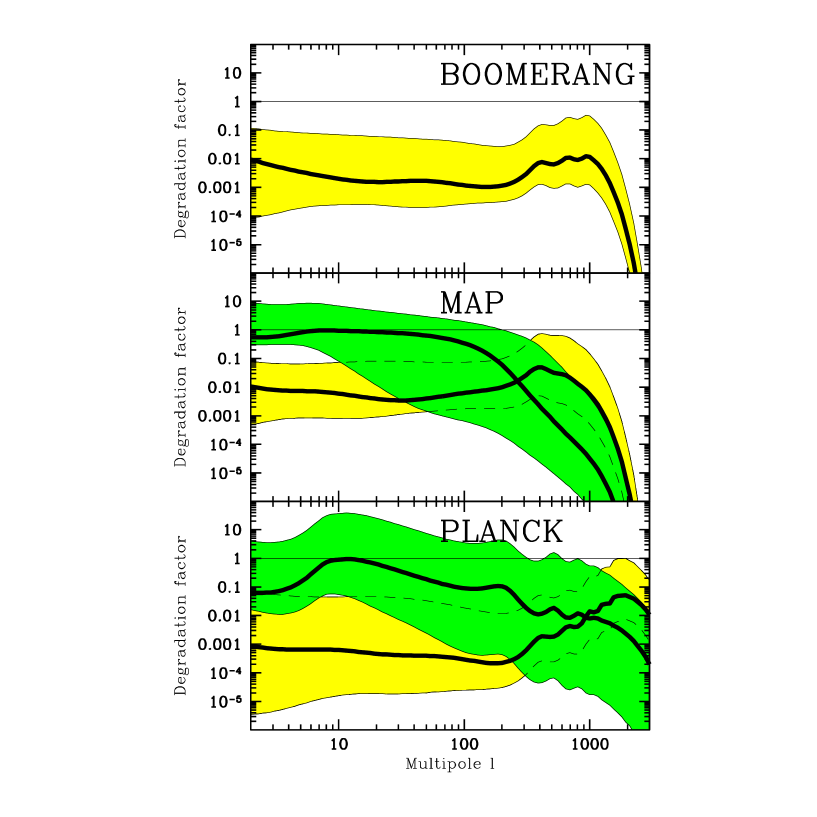
Two other foreground degradation measures have been previously used in the literature. The most closely related one is the foreground degradation factor of Dodelson (1996), which is the ratio of the rms noise in the cleaned maps for the cases with and without foregrounds. This assumed that foregrounds could be subtracted out completely, i.e., that $\Delta\alpha=0$ and that there were more components channels than foregrounds. The “quality factor” (Bouchet et al. 1999; BG99) is the amount by which multifrequency Wiener filtering suppresses the power of the CMB in the cleaned map, assuming $\Delta\alpha=0$, and was defined for each foreground component separately. The most important difference is that our degradation factor is relative to the noise plus sample variance, since our focus is on power spectra and measurement of cosmological parameters.

4.5. Dependence on assumptions about amplitude

The MID model in Figure 11 gives our estimate of how small the noise and foreground power spectra can be made in the cleaned maps, while comparing the OPT and PESS models indicates the range of uncertainty. Let us now discuss the effects of model assumptions in more detail.

The foreground behavior enters in two different ways:

1. The assumed foreground behavior determines the weights ${\bf w}$ that we use when cleaning the maps.

2. The true foreground behavior determines the actual foreground residual in the cleaned maps.

Let us make this distinction explicit by using ${\mathcal{N}}_{a}$ to denote our assumed foreground matrix (our prior), as distinguished from the true matrix ${\mathcal{N}}$. The resulting foreground contamination is then given by (suppressing the $\ell$ subscript)

$${\bf\Sigma}=[{\mathcal{A}}^{t}{\mathcal{N}}_{a}^{-1}{\mathcal{A}}]^{-1}[{\mathcal{A}}^{t}{\mathcal{N}}_{a}^{-1}{\mathcal{N}}{\mathcal{N}}_{a}^{-1}{\mathcal{A}}][{\mathcal{A}}^{t}{\mathcal{N}}_{a}^{-1}{\mathcal{A}}]^{-1},$$ (49)

which only reduces to equation (40) if ${\mathcal{N}}_{a}={\mathcal{N}}$, i.e., if our model is correct. We will still recover unbiased CMB maps $T$, $E$ and $B$ even if our model is incorrect, but generally with larger foreground contamination than would be attainable with a correct model.

Equation (49) shows that the contaminant power spectra in ${\bf\Sigma}$ depend linearly on ${\mathcal{N}}$. Thus the complicated residual foreground power spectra depicted in the 3 rightmost panels of Figures 1–6 (computed equation (49) by taking ${\mathcal{N}}$ to be the contribution from a single foreground component) may be thought of as the result of multiplying the rather featureless foreground power spectra that are actually on the sky by known transfer functions.

4.6. Dependence on assumptions about frequency coherence

4.6.1 Effect of changing $\Delta\alpha$

Figure 12.— The effect of frequency coherence. The total power spectrum from noise and foregrounds in the cleaned Planck $T$ map is shown for five different assumptions about frequency coherence, corresponding to multiplying all values of $\Delta\alpha$ from the MID model (heavy curve) by $\infty$, 2, 1, 0.5 and 0, respectively (from top to bottom). The fiducial CMB power spectrum is shown for comparison.

Figure 13.— The weights ${\bf w}_{\ell}^{T}$ with which the unpolarized maps at the 9 Planck frequencies are combined into a single map are plotted as a function of angular scale $\ell$ for the MID model, but with completely incoherent foregrounds ($\Delta\alpha=\infty$).

Figure 14.— The weights ${\bf w}_{\ell}^{T}$ with which the unpolarized maps at the 9 Planck frequencies are combined into a single map are plotted as a function of angular scale $\ell$ for the MID foreground model.

Figure 15.— The weights ${\bf w}_{\ell}^{T}$ with which the unpolarized maps at the 9 Planck frequencies are combined into a single map are plotted as a function of angular scale $\ell$ for the MID model, but with perfectly coherent foregrounds ($\Delta\alpha=0$).

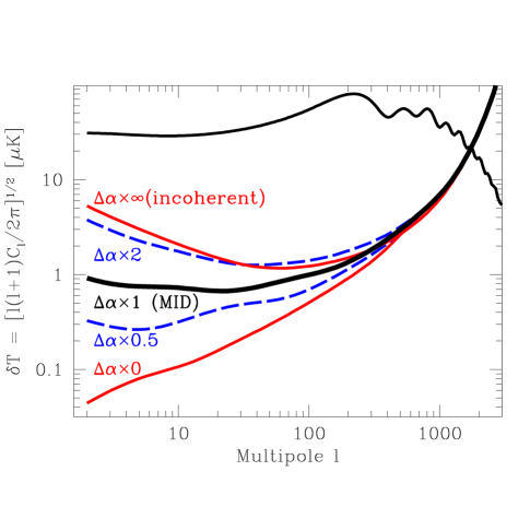
In general, the less coherent a foreground is, the more difficult it is to remove. Figure 12 shows this effect. All panels use the scale and frequency dependence of the MID model, but with the frequency coherence spanning the range between the extreme cases $\xi=\infty$ and $\xi=0$. As expected, the situation generally gets worse as we progress from ideal perfectly coherent foregrounds (bottom curve) to realistic (middle three curves) and completely incoherent ones (top curve), The incoherent case corresponds to no foreground subtraction whatsoever, simply averaging the Planck channels with inverse-variance weighting.

While less coherence is usually a bad thing, Figure 12 shows a subtle exception to this rule at $\ell\sim 100$. Here weak coherence is seen to be worse than no coherence at all. Figures 13-15 shed more light on this perhaps surprising behavior by showing how the channel weighting changes as we increase the frequency coherence. These figures correspond to three of the five curves in Figure 12 (the top, middle and bottom ones). Figure 13 shows the case of completely incoherent foregrounds ($\Delta\alpha=\infty$). It gives an inverse-variance weighting just as in Figure 9, but with the variance receiving a contribution from foregrounds as well as noise. In Figure 14, we see that the poor coherence between widely separated channels is forcing the method to do much of the foreground subtraction using neighboring channels, using costly large-amplitude weights at 100, 143 and 217 GHz on large scales. In contrast, the case of ideal foregrounds shown in Figure 15 is seen to be much easier to deal with, requiring no weights exceeding unity in amplitude. For instance, the small dust contribution at low frequencies can be subtracted out essentially for free, by a tiny negative weight for the dust-dominated 545 GHz channel.

The non-monotonic behavior (where things eventually start improving again when the coherence becomes sufficiently low) does not occur if there is merely a single foreground component present with no detector noise. Instead, it results from an interplay between foregrounds and noise. A perfectly incoherent foreground can be efficiently dealt with in the same way as noise: by inverse-variance weighting the channels as in Figure 13, the incoherent foreground fluctuations will average down, whereas a coherent foreground would not. Typically, the worst case is for $\xi$ of order unity, although the exact value depends on the other foregrounds. Figure 12 thus shows that although we do not appear to live in the worst of all possible worlds, we are only off by a small factor!

4.6.2 Effect of incorrect assumptions about $\Delta\alpha$

Figure 16.— The effect of faulty assumptions about frequency coherence. The total power spectrum from noise and foregrounds in the cleaned Planck $T$ map is shown for the MID model using three different assumptions for the cleaning process: the correct (MID) $\Delta\alpha$-values (bottom), $\Delta\alpha=\infty$ (middle, cautious) and $\Delta\alpha=0$ (top, foolhardy). The fiducial CMB power spectrum is shown for comparison.

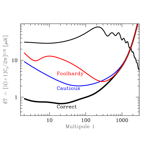
What if our model is incorrect? Figure 16 uses equation (49) to show the effect of two kinds of errors: being too optimistic and being too pessimistic about ones abilities to model the frequency dependence of foregrounds. For all there curves, the MID model is used as the truth, but the weights ${\bf w}$ for the foregrounds subtraction are for different assumptions about the frequency coherence. Not surprisingly, correct assumptions give the best removal, showing the importance of accurately measuring the actual frequency coherence of foregrounds. The curve labeled “cautious” shows the result of assuming incoherent foregrounds ($\Delta\alpha=\infty$), corresponding to no foreground subtraction at all, merely inverse-variance averaging with no negative weights as in Figure 13) whereas the one labeled “foolhardy” illustrates the effect of assuming ideal foregrounds ($\Delta\alpha=0$, using the weights of Figure 15). The fact that the former generally lies beneath the latter shows that when faced with uncertainty about $\Delta\alpha$, it is better to err on the side of caution: in our example, foreground removal based on the overly optimistic model is performing worse than no foreground removal at all.

4.6.3 Effect of functional form of coherence

Figure 17.— Changing the functional form of frequency coherence. The total power spectrum from noise and foregrounds in the cleaned Planck $T$ map is shown for the MID model using different shapes for the coherence function $f$, shown with the corresponding line type in the inset. The shapes are Gaussian (heavy solid curve), Lorentzian (short-dashed), exponential (thin solid curve), flat (dotted) and completely incoherent (long-dashed). The fiducial CMB power spectrum is shown for comparison.

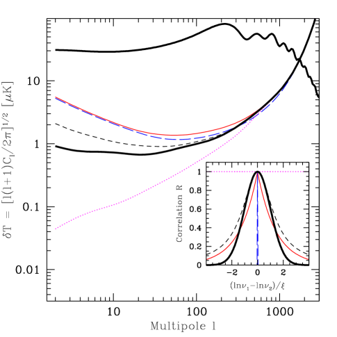
We can rewrite our coherence model of equation (25) as

$${\bf R}_{(k)}^{Pf{f^{\prime}}}=f\left(\ln\nu_{f}-\ln\nu_{f^{\prime}}\over\xi_{(k)}^{P}\right),$$ (50)

where $f(x)=e^{-x^{2}/2}$. The derivation in T98 did not show that $f(x)$ was a Gaussian, merely that behaved like a parabola at the origin with $f(0)=1$, $f^{\prime}(x)=0$ and $f^{\prime\prime}(0)=-1$. Since $f$ (which we will term the coherence function) has not yet had its shape accurately measured for any foreground, we repeat the Planck analysis for a variety of such functions of the form

$$f(x)=\left(1+{x^{2}\over 2n}\right)^{-n}.$$ (51)

The case $n=\infty$ recovers the Gaussian of equation (25), $n=1$ gives a Lorentzian, etc.

Figure 17 shows that the shape of the far wings of $f$ is only of secondary importance—the main question is how correlated neighboring channels are, which for $\xi\gg 1$ depends mainly on the curvature of $f$ near the origin. Narrowing the wings (increasing $n$) usually helps slightly, once again demonstrating that more coherence is not necessarily a good thing. For comparison, Figure 17 shows the case where $f(x)=1$ at the origin and vanishes elsewhere and the case $f(x)=1$, corresponding to the limits $\Delta\alpha=\infty$ and $\Delta\alpha=0$, respectively. Also shown is the exponential coherence function $f(x)=\exp[|x|/\sqrt{(}2)$. This is seen to be quite a conservative choice, giving even larger residuals than the $\Delta\alpha=\infty$ case, since the correlations between neighboring channels are strong enough to be important but not good enough to be really useful for foreground subtraction. A generalization of this exponential coherence function will come in handy in §5, where our goal is to be as pessimistic as possible with the intent to destroy parameter estimation with foregrounds.

5. Simultaneous Estimation of Foregrounds and Cosmology

To this point, we have considered the case in which the statistical properties of the foregrounds are known exactly. Moreover we have shown that incorrect assumptions about these properties can lead to foreground removal strategies that do more harm than good. This begs the question of whether we will in fact know these foregrounds to the level needed for accurate subtraction. The sky maps from CMB satellite missions will provide some of the most relevant data on this question. Hence, we will next consider the case in which cosmological parameters and the foreground model are simultaneously estimated from the CMB data.

At this point, the calculation becomes less well-defined. If we are allowed to consider arbitrary excursions around the fiducial model, then cosmological parameter estimation fails completely. There is no mathematical way to exclude a foreground that matches the CMB frequency dependence, is perfectly coherent, and has an arbitrarily inconvenient power spectrum (say, one mimicking the variation of a cosmological parameter). Physically, however, we believe this to be unreasonable. We therefore must construct a parameterized model of foregrounds that allows for a reasonably, but not completely, general coverage of the possibilities.

5.1. Cosmological Parameters

We adopt a low-density, spatially flat adiabatic CDM model for our cosmology. The model has a matter density of $\Omega_{m}=0.35$, a baryon density of $\Omega_{b}=0.05$, a massive neutrino density of $\Omega_{\nu}=0.0175$ (one massive species with a mass of $0.7{\rm\ eV}$), and a cosmological constant $\Omega_{\Lambda}=0.65$. The primordial helium fraction is $Y_{P}=0.24$. The Hubble constant is $H_{0}=100h{\rm\ km\ s^{-1}\ Mpc^{-1}}=65{\rm\ km\ s^{-1}\ Mpc^{-1}}$. The universe is reionized suddenly at low redshift with an optical depth of $\tau=0.05$. The primordial power spectrum is scale-invariant, so the scalar spectral index is $n_{S}=1$. There are no tensors ($T/S=0$). The model is normalized to the COBE-DMR experiment. This is the same model that was used in Eisenstein et al. (1999, hereafter “E99”), and further details on the above choices can be found there.

We will ask how well CMB data can constrain a 10-dimensional excursion around this parameter space. The parameters are $\Omega_{m}h^{2}$, $\Omega_{b}h^{2}$, $\Omega_{\nu}h^{2}$, $\Omega_{\Lambda}$, $\tau$, $Y_{P}$ (constrained to vary by 0.02 at 1-$\sigma$), $n_{S}$, $n_{S}^{\prime}$, $T/S$, and the normalization. $ns^{\prime}$ (denoted $\alpha$ in E99) is the running of the scalar tilt,

$$n_{S}(k)=n_{S}(k_{\rm fid})+n_{S}^{\prime}\ln(k/k_{\rm fid}),$$ (52)

where $k_{\rm fid}=0.025{\rm\,Mpc}^{-1}$. Note that $\Omega_{m}=1-\Omega_{\Lambda}$ and $h=\sqrt{(\Omega_{m}h^{2})/(1-\Omega_{\Lambda})}$ are defined implicitly and hence can vary. This parameter space is identical to that of E99 except that we have not included spatial curvature. There is a severe degeneracy between curvature and the cosmological constant (Bond et al. 1997; Zaldarriaga et al. 1997). Since this degeneracy is best broken by using non-CMB data (e.g., galaxy redshift surveys or SN Ia), we choose to focus only on the well-constrained combination of the two parameters here. Details of how we perform the numerical derivatives of the power spectra with respect to these cosmological parameters can be found in E99. Fortunately, all the derivatives with respect to the foregrounds (§5) can be done analytically, so that no new numerical problems are introduced.

5.2. Foreground Parameters

We allow for uncertainty in the foregrounds by adding a large number of parameters to the models specified in §2. Recall that each component was specified by a frequency dependence, a frequency coherence, and a power spectrum for each polarization type ($T$, $E$, $B$, and $X$). For each type and each component, we now include parameters to allow excursions in frequency dependence, frequency coherence, and spatial power. As described below, we use of order fifty additional parameters denoted by vectors ${\mathbf{q}}$, ${\mathbf{r}}$ and ${\mathbf{s}}$ for each foreground component.

For the frequency dependence, we allow a piecewise power-law excursion in thermodynamic temperature around the fiducial model

$$\ln\Theta_{(k)}^{P}(\nu)=\left.\ln\Theta_{(k)}^{P}(\nu)\right|_{\rm fid}+L\left(\ln\nu;{\mathbf{q}}_{(k)}^{P}\right).$$ (53)

Here, the function $L$ is a linear interpolation between the values $({\mathbf{q}}=q_{1},\ldots,q_{n_{\nu}})_{(k)}^{P}$ at the breakpoints $\nu^{1},\ldots,\nu^{n_{\nu}}$, so $L(\ln\nu^{i};{\mathbf{q}}_{(k)}^{P})=q_{i(k)}^{P}$ and is a straight line between breakpoints and the fiducial model (“fid”) has ${\mathbf{q}}_{(k)}^{P}=0$. This means that we can rewrite it as

$$L(\ln\nu;{\mathbf{q}})=\sum_{i=1}^{n_{\nu}}q_{i}L_{i}(\ln\nu),$$ (54)

where the functions $L_{i}$ have triangular shape as illustrated in Figure 18: $L_{i}(\ln\nu^{i})=1$, goes linearly to zero at the neighboring breakpoints, and vanishes everywhere else.

Figure 18.— The figure shows the four triangle functions $L_{i}$ that span the excursions in frequency dependence for foregrounds seen by MAP. Any function that is piecewise linear between the four break points (e.g., the heavy curve) can be written as a linear combination of these functions in this range.

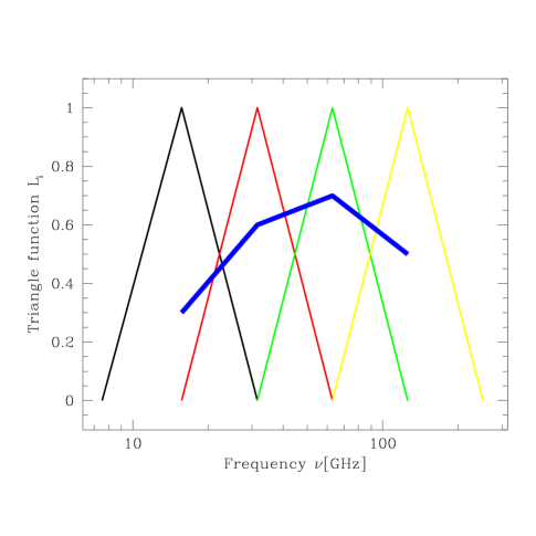
We allow a separate frequency excursion for $T$, $E$, and $B$ for each foreground component. For the cross correlation we allow for the possibility that the excursions in the correlation of the temperature at $\nu$ and $E$-polarization at $\nu^{\prime}$ is not the same as the temperature at $\nu^{\prime}$ with the $E$-polarization at $\nu$. We therefore define two excursions for the cross-correlation ${\mathbf{C}}_{\ell(k)}^{X}(\nu,\nu^{\prime})\propto\Theta_{(k)}^{X_{T}}(\nu)\Theta_{(k)}^{X_{E}}(\nu^{\prime})$. One of the excursions affects the temperature index, the other the polarization index. $\left.\Theta_{(k)}^{X_{T}}\right|_{\rm fid}=\Theta_{(k)}^{X}$ and likewise for ${X_{E}}$ since we have assumed that the fiducial model is symmetric in this respect.

Since the breakpoints $\nu^{i}$ specify the degrees of freedom in the foreground model, they are independent of the number and location of observing frequencies $\nu_{i}$ for any given experiment. We choose them to be evenly spaced in $\ln\nu$, with a factor of 2 in frequency between each, and are centered at the geometric mean of the highest and lowest frequencies of the experiment. This means that we specify $n_{\nu}=4$ breakpoints for Boomerang (67.1, 134, 268, and 537 GHz) and MAP (15.7, 31.5, 62.9, and 126 GHz) and $n_{\nu}=6$ for Planck (28.3, 56.7, 113, 227, 454, 907 GHz).

In the $n_{\nu}=2$ limit, the new parameters correspond to varying the normalization and power-law exponent of the frequency dependence of the foreground component. We chose to extend this freedom by piecewise-linear interpolation rather than smoother options for technical reasons. Splines have non-local behavior; frequencies far outside the range of the CMB experiment would affect the results inside the range. Polynomials are scale-free, so that a polynomial of a given order will adapt itself to the particular experimental specifications so as to put the maximal number of wiggles inside the frequency range. This would mean that the effective number of degrees of freedom in the foreground model would not be consistent from one experiment to the next. Simple interpolation avoids these problems: one need not specify any breakpoints beyond the first outside the frequency range of the experiment, and the scale for variations in the foreground is independent of the experiment.

We don’t allow frequency variations for the thermal SZ component, because its spectrum is theoretically known. As discussed in §2.4, relativistic corrections are expected to be negligible for filaments, so we ignore this complication.

To include these parameters in the Fisher matrix of equation (22), we must specify the derivatives of ${\mathcal{C}}_{\ell}$ with respect to the interpolation parameters ${\mathbf{q}}_{(k)}^{P}$. Clearly only the elements of the same component and polarization type are affected. For $P=T$, $E$, and $B$, the derivatives of that submatrix are

$$\left.{\partial C_{\ell(k)}^{Pf{f^{\prime}}}\over\partial q_{i(k)}^{P}}\right|_{\rm fid}=C_{\ell(k)}^{Pf{f^{\prime}}}\left[L_{i}(\ln\nu_{f})+L_{i}(\ln\nu_{f^{\prime}})\right],$$ (55)

where we have used equation (54). For $P=X$, the derivatives are

$${\partial C_{\ell(k)}^{Xf{f^{\prime}}}\over\partial q_{i(k)}^{X_{T}}}=C_{\ell(k)}^{Xf{f^{\prime}}}L_{i}(\ln\nu_{f}),$$ (56)

$${\partial C_{\ell(k)}^{Xf{f^{\prime}}}\over\partial q_{i(k)}^{X_{E}}}=C_{\ell(k)}^{Xf{f^{\prime}}}L_{i}(\ln\nu_{f^{\prime}}).$$ (57)

For the frequency coherence, we adopt the exponential model for the matrix ${\mathbf{R}}$ using

$${\mathbf{R}}^{f{f^{\prime}}}=\exp\left[-\left|\int^{\nu_{f^{\prime}}}_{\nu_{f}}\,\Delta(\nu)d(\ln\nu)\right|\right].$$ (58)

In the fiducial model, $\Delta(\nu)=\Delta\alpha=1/\sqrt{2}\xi$ independent of frequency. Now we allow excursions of the form

$$\Delta(\nu)=\Delta\alpha+L(\ln\nu;{\mathbf{r}}),$$ (59)

where $L$ is a linear interpolation function as before, parameterized by ${\mathbf{r}}=r_{1},\ldots,r_{n_{\nu}}$. We use the same spacing of the interpolation points $\nu^{1},\ldots,\nu^{n_{\nu}}$ as in the frequency dependence case described above.

As above, for each foreground component except SZ, we allow separate excursions for each of $T$, $E$, and $B$ and two excursions for $X$. The derivatives of ${\mathcal{C}}$ are ($P=T$, $E$, $B$)

$${\partial C_{\ell(k)}^{Pf{f^{\prime}}}\over\partial r_{i(k)}^{P}}=-C_{\ell(k)}^{Pf{f^{\prime}}}\left|\int^{\nu_{f^{\prime}}}_{\nu_{f}}\,d(\ln\nu)L_{i}(\ln\nu)\right|.$$ (60)

For the cross-correlation $X$, we allow for an asymmetric excursion by invoking two excursions of the above form and setting either the upper ($f<{f^{\prime}}$) or lower ($f>{f^{\prime}}$) triangle elements to zero.

For the spatial power, we consider excursions of the form

$$\ln C_{\ell(k)}^{P}=\left.\ln C_{\ell(k)}^{P}\right|_{\rm fid}+L(\ln\ell;{\mathbf{s}}),$$ (61)

where $L$ is a linear interpolation function. The parameters ${\mathbf{s}}=s_{1},\ldots,s_{n_{\ell}}$ are the values of $L$ at a grid of $\ell$ that begins at $\ell=2$ and increased by factors of $e$. As we sum the Fisher contribution to $\ell_{\rm max}=2800$, this gives $n_{\ell}=9$ grid points. However, the overall normalization (i.e. moving all the $s_{i}$ the same amount) is degenerate with an overall shift in the frequency dependence (eq. [53]), so in cases other than the thermal SZ, we hold the middle spatial $s_{j}$ ($\ell=109$) equal to zero.

Separate excursions are allowed in $P=T$, $E$, $B$, and $X$ for each foreground component, including the SZ effect. The derivatives of ${\mathcal{C}}$ with respect to these parameters are

$${\partial{\mathbf{C}}_{\ell(k)}^{P}\over\partial s_{i(k)}^{P}}={\mathbf{C}}_{\ell(k)}^{P}L_{i}(\ln\ell),$$ (62)

where all terms involving different $k$ and $P$ are zero, as before. The $L_{i}$ spatial functions are defined analogously to equation (54).

In short, for most foreground components, we have $10n_{\nu}+4n_{\ell}-4$ free parameters in $({\mathbf{q}},{\mathbf{r}},{\mathbf{s}})$. For the thermal SZ, we have only $4n_{\ell}$. However, for unpolarized components, the parameters for polarization excursions have zero derivatives, so we remove them. This leaves 385 (489) parameters for MAP (Planck) for the MID model, 257 (325) for the OPT model, and 441 (561) for the PESS model. For the MID model, 105 (129) of the parameters are associated with the intensity anisotropies, so there are 105 parameters for our Boomerang estimates.

We allow these parameters to vary without external priors in almost all cases. As we will show below, the CMB experiments are able to constrain the foreground model well enough to extract the cosmic signal. The one exception is the thermal SZ effect with the MAP experiment. The frequency dependence of the SZ is similar to the cosmic temperature variations for frequencies much below 200 GHz. If we allow unfettered variations in the SZ spatial power spectrum, there are significant degradations in the performance of MAP on cosmological parameters. However, these degeneracies correspond to very large departures from the fiducial SZ level. We therefore include a prior (for MAP only) that the SZ power spectrum cannot vary by more than a factor of 10 from the fiducial level (i.e., the parameters $z_{i}$ cannot exceed 10 at 1-$\sigma$ confidence). This is an extremely generous prior—numerical simulations are surely correct to within a factor of 10 at 68% confidence—but it substantially reduces the degradation of the MAP performance in the presence of SZ signals. In detail, for the MID model, MAP with $T$ alone could measure $\Omega_{b}h^{2}$ to 0.0036 with the SZ variations being omitted, 0.0037 with the prior described above, and 0.0075 with a prior of $10^{6}$ on the SZ variations. For this and other parameters, the prior of 10 removes variations in the SZ as a source of cosmological uncertainty in the MID model. The PESS model, with its 10-fold increase in the fiducial SZ level, has 10-20% differences between results with a prior of 10 and those with no SZ variations. Planck and Boomerang can control the SZ to better than a factor of 10, so no prior is applied.

5.3. Cosmological Parameters in the Presence of Foregrounds

Because the variations in the foreground model have effects at all $\ell$, we cannot express the effects of the foregrounds as a simple degradation of the error bars at each multipole (c.f. Fig. 11). Excursions from the fiducial model produce changes in frequency and scale dependence that can compensate both each other and cosmological signals in complicated ways. In other words, with this more complicated foreground model, one does not recover a cleaned CMB power spectrum as an intermediate step of the analysis, but must proceed directly to the estimation of the parameters characterizing the models for foregrounds and cosmology. To quantify the effects of the foregrounds, we will therefore simply compare the final marginalized error bars on cosmological parameters.

Table 3

Marginalized Errors with Foreground Variations
Foregrounds Experiment Quantity None Known Unknown Boomerang (T) $\ln(\Omega_{m}h^{2})$ 0.45 1.007 1.282 $\ln(\Omega_{b}h^{2})$ 0.27 1.008 1.242 $m_{\nu}$ (eV) $\propto\Omega_{\nu}h^{2}$ 3.5 1.006 1.51 $n_{S}(k_{\rm fid})$ 0.30 1.007 1.203 $\Omega_{\Lambda}$ 0.57 1.007 1.287 $\tau$ 1.3 1.016 1.87 $T/S$ 1.2 1.007 1.52 MAP (T) $\ln(\Omega_{m}h^{2})$ 0.20 1.027 1.393 $\ln(\Omega_{b}h^{2})$ 0.12 1.027 1.453 $m_{\nu}$ (eV) $\propto\Omega_{\nu}h^{2}$ 0.87 1.017 1.65 $n_{S}(k_{\rm fid})$ 0.11 1.026 1.332 $\Omega_{\Lambda}$ 0.23 1.026 1.324 $\tau$ 0.31 1.014 1.69 $T/S$ 0.42 1.023 1.240 MAP (TP) $\ln(\Omega_{m}h^{2})$ 0.080 1.208 1.66 $\ln(\Omega_{b}h^{2})$ 0.051 1.201 2.01 $m_{\nu}$ (eV) $\propto\Omega_{\nu}h^{2}$ 0.57 1.078 2.06 $n_{S}(k_{\rm fid})$ 0.041 1.264 2.63 $\Omega_{\Lambda}$ 0.091 1.230 1.74 $\tau$ 0.018 1.90 3.33 $T/S$ 0.16 1.309 1.86 Planck (T) $\ln(\Omega_{m}h^{2})$ 0.062 1.014 1.042 $\ln(\Omega_{b}h^{2})$ 0.035 1.013 1.040 $m_{\nu}$ (eV) $\propto\Omega_{\nu}h^{2}$ 0.55 1.010 1.029 $n_{S}(k_{\rm fid})$ 0.041 1.013 1.031 $\Omega_{\Lambda}$ 0.080 1.013 1.039 $\tau$ 0.23 1.015 1.074 $T/S$ 0.18 1.011 1.035 Planck (TP) $\ln(\Omega_{m}h^{2})$ 0.016 1.056 1.160 $\ln(\Omega_{b}h^{2})$ 0.0094 1.028 1.165 $m_{\nu}$ (eV) $\propto\Omega_{\nu}h^{2}$ 0.24 1.032 1.075 $n_{S}(k_{\rm fid})$ 0.0076 1.109 1.303 $\Omega_{\Lambda}$ 0.022 1.051 1.151 $\tau$ 0.0036 1.69 1.96 $T/S$ 0.0073 4.04 6.58

NOTES.—Marginalized errors for some cosmological parameters within the 12-dimensional adiabatic CDM family of cosmological models and the exponential coherence function (eq. [58]) for the foregrounds. “None” column lists $1-\sigma$ error in case where there are no foregrounds. “Known” column lists the relative degradation when our foreground MID model is added under the assumption that the statistical properties of the foregrounds are known exactly. “Unknown” column lists the relative degradation when the statistical properties of the foregrounds must be simultaneously estimated within a generous parameterization of possible models. Results for MAP with intensity only (T) and with intensity and polarization (TP) are shown; likewise for Planck. $n_{S}(k_{\rm fid})$ is the logarithmic derivative of the scalar primordial power spectrum at $k_{\rm fid}=0.025{\rm\,Mpc}^{-1}$; in the presence of $n_{S}^{\prime}\neq 0$, $n_{S}$ is a function of scale. Cosmological model is $\Omega_{m}=0.35$, $\Omega_{b}=0.05$, $\Omega_{\nu}=0.0175$ ($m_{\nu}=0.7{\rm\ eV}$), $\Omega_{\Lambda}=0.65$, $h=0.65$, $n_{S}=1$, $n_{S}^{\prime}=0$, $\tau=0.05$, $Y_{p}=0.24$, and $T/S=0$. $n_{T}=0$ and cannot vary.

For display purposes, we will focus on the performance on four parameters, chosen to illustrate important aspects of the interplay between foregrounds and cosmological signals:

1. The baryon density $\Omega_{b}h^{2}$ as measured only from the temperature information. This parameter is sensitive to the structure of the acoustic peaks and to the diffusion scale (Hu & Sugiyama 1995).

2. $\Omega_{b}h^{2}$ as measured from both intensity and polarization. The polarization of the acoustic peaks substantially improve the accuracy with which this parameter can be measured (Zaldarriaga et al. 1997) — mainly through the X power spectrum, as we will see in §5.4.5.

3. The reionization optical depth $\tau$ as measured from intensity and polarization. This is dominated by the $E$-channel signal at large angular scales (Hogan et al. 1982), thereby testing how well the diffuse polarized galactic signals can be removed.

4. The tensor-to-scalar ratio $T/S$ as measured from intensity and polarization. This is the only cosmic signal in the B-channel polarization (Kamionkowski et al. 1997; Zaldarriaga & Seljak 1997).

Figure 19.— Relative degradation in error bars from MAP on four cosmological parameters as the amplitude of foregrounds are increased. (top-left) Behavior of $\Omega_{b}h^{2}$ with intensity information only (T). (proceeding clockwise) $\Omega_{b}h^{2}$, $T/S$, and $\tau$ with intensity and polarization information (TP). Bars show the error bar for each foreground case relative to the no-foregrounds case; the $1-\sigma$ error of the latter is listed in each panel. The histograms show results for a series of foreground models, ranging from no foregrounds to our OPT, MID, and PESS models. (lightly-shaded) Results with foregrounds of known properties. (heavily-shaded) Results with foregrounds whose parameters must be simultaneously estimated from the CMB data.

Figure 20.— As Figure 19, but for Planck.

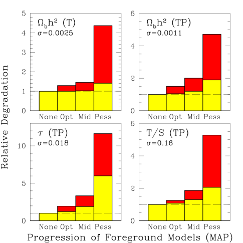
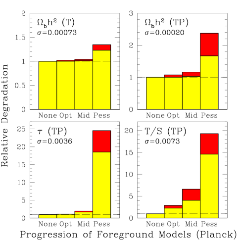
In Figures 19 and 20, we show the degradation of the MAP and Planck performance on these parameters in the presence of our OPT, MID, and PESS foreground models. In each case, the baseline is the performance in the absence of any foregrounds at all. The degradations in the presence of foregrounds are shown for both the case of known properties and the case of unknown properties.

The performance on $\Omega_{b}h^{2}$ with and without polarization is very encouraging. The degradations are less than a factor of 2 in all cases but the PESS model in MAP (where it reaches 4-5). Planck is able to survive even the PESS model with only a factor of 2 increase in the projected errors. The reason for this strong performance is the detailed structure of the acoustic peaks. Even if cleaning is imperfect, the foreground power spectra do not have the oscillatory behavior of the cosmic derivatives and can therefore be distinguished from variations in cosmological parameters. Note that most of the degradation can be attributed to uncertainties in the foreground model; the performance in the case of known foreground properties is nearly perfect.

The situation is somewhat less rosy for the large-angle polarization signals. $\tau$ and $T/S$ both have unique signatures in the large-angle polarization, where signals from the acoustic peaks are quite weak. In the absence of foregrounds, even small cosmic signals can be detected because their sample variance is equally low. With foregrounds, the signal-to-noise is considerably worse. Performance is correspondingly poorer, and the results do depend more sensitively on the severity of the foregrounds. However, one should note that for the OPT and MID models, even the large-angle polarization signal can be cleaned to reasonable accuracy, yielding excellent constraints on $\tau$ and $T/S$. For the PESS model, the degradation is generally more than a factor of 10, although the errors for Planck would still be interesting ($\sim\!5\%$ for $\tau$, $\sim\!10\%$ for $T/S$).

Note that the extra frequency coverage and sensitivity of Planck does not imply that it will necessarily suffer less relative degradation than MAP from the presence of foregrounds; although Planck will clean more effectively, its baseline projections were more ambitious.

In Table 3, we display the numerical results for Boomerang, MAP, and Planck with the MID foreground model. The errors without foregrounds are shown, followed by the relative degradations in the presence of foregrounds with and without knowledge of their properties. For the satellites, we show results considering intensity information alone and then both intensity and polarization information. Boomerang is slightly more robust against foregrounds than MAP, reaching 3-fold degradations in the PESS model. Because our foreground model has more components centered at lower frequencies, the higher frequency range of Boomerang may shift it away from the reach of the model’s variations.

5.4. Which details matter?

Figure 21.— As Figure 19, but increasing the diffuse foregrounds and point sources separately. “Mid” bars refer to the MID foreground model, simultaneously estimating the foreground parameters. “Diff” bars show the results when the diffuse components (i.e. all those that are not point sources) are increased by 10 in amplitude. “PS” bars show the results when the point source and SZ components have their amplitude (after PSF fitting) increased by a factor of 10. “$\times 10$” bars show the combined result. All values are shown as the fractional increase relative to the results with no foregrounds. This figure shows the case for MAP.

Figure 22.— As Figure 21, but for Planck.

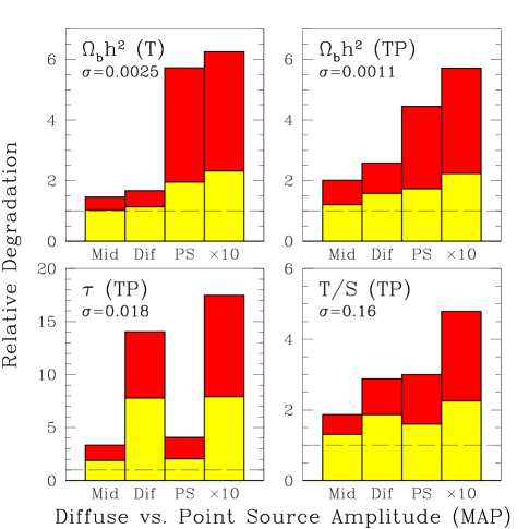
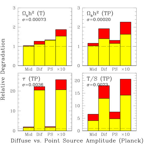
5.4.1 Dependence on foreground amplitude

As we increase the amplitudes of the foregrounds, which components most affect which cosmological parameters? We consider artificially boosting the amplitudes of the MID foreground model by a factor of 10 (i.e., a factor of 100 in power). In Figures 21 and 22, we apply this factor of 10 increase separately to the diffuse components and to the SZ and point source components. Generally, the errors on $\tau$ and $T/S$ are primarily affected by the diffuse components rather than the point sources, while the results for $\Omega_{b}h^{2}$ are the reverse. However, there are some mild exceptions. For Planck with polarization, $\Omega_{b}h^{2}$ is sensitive to the amplitude of the diffuse components. This is because we assumed the power spectrum of the polarization of dust and synchrotron to be considerably bluer than that of the intensity. Hence, when increased in amplitude, these foregrounds contaminate the acoustic peak structure in the polarization and degrade the performance somewhat. Also, for MAP  the results on $T/S$ are sensitive to both diffuse and point-source components. MAP does not make a strong detection of the tensor signal in the polarization and is therefore reliant upon the large-angle signal in the intensity. Boosting the point source amplitude confuses the comparison between $\ell\approx 50$ and $\ell\approx 500$ that would test for the presence of tensors. The trends in Figures 21 and 22 are insensitive to whether foreground parameters are assumed to be known or not.

5.4.2 Dependence on frequency coherence

As was discussed in §4.6.1, the cleaning of foregrounds is usually more effective when a map at one frequency gives a good estimate of the foreground’s presence at another frequency. This is governed by the covariance matrix $R$ and the frequency coherence $\Delta\alpha$. Because the parameters of this matrix are very poorly known at the present time, it is important to check that our results are insensitive to our choices in this sector.

As described above, the parameter $\Delta\alpha$ sweeps between the two extremes of perfect correlation between frequency channels and total independence. As shown in T98, both of these cases have desirable properties for removal of foregrounds. In the former case, there is a particular combination of the frequency maps that completely removes the component in question. In the latter case, one uses the fact that any correlation between different maps must be cosmic signal. Of course, neither perfect correlation nor total independence is correct, and the intermediate case admits a less complete cleaning of foregrounds.

Figure 23.— As Figure 19, but altering the frequency coherence $\Delta\alpha$ of the fiducial foreground model. We scale all $\Delta\alpha$ (see Table 2) by a factor of 0, 0.3, 1, 3, 10, and $\infty$. As shown in T98, perfect coherence and perfect decoherence are the best-cases; intermediate values yield worse performance. All errors are shown relative to those in the case with no foregrounds.

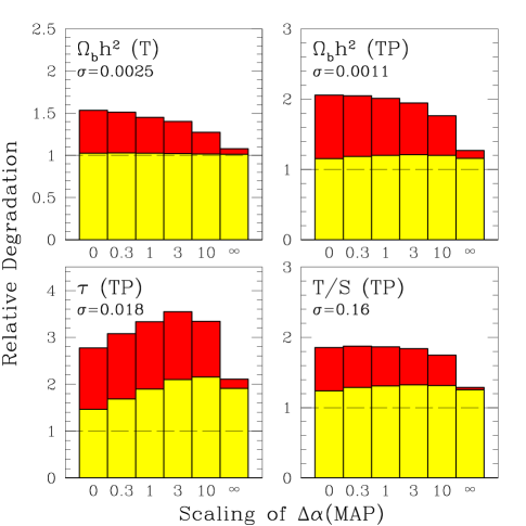
In Figures 23 and 24, we show a sequence of models in which we scale all of the $\Delta\alpha$’s in the MID model by a constant that ranges from zero (perfect correlation) to $\infty$ (complete independence). As expected, the errors on cosmological parameters increase as one moves away from the extremes and reaches a maximum in the middle. This peak typically occurs when the $\Delta\alpha$’s of the foregrounds are multiplied by $\sim\!3$, but the actual location varies from case to case. However, because the peak is broad, the errors from our base model are actually rather close to the maximum. We therefore conclude that our treatment of the covariance between the frequency channels has been sufficiently conservative.

5.4.3 Dependence on foreground model complexity

We now consider turning off certain sets of variations to examine which variations are causing the most degradation. The results are shown in Table 4. We separate the foreground parameters into three sets, namely those involving the frequency dependence (the ${\mathbf{q}}_{(k)}^{P}$), the frequency coherence (the ${\mathbf{r}}_{(k)}^{P}$), and the spatial power spectrum (the ${\mathbf{s}}_{(k)}^{P}$). By convention, the overall normalization of the foreground component is carried by the frequency dependence, not the spatial power spectrum. We include these sets one at a time and in pairs to investigate which is most important. Considered singly, uncertainties in the shape of the power spectrum generally increase the error bars the most, although uncertainties in frequency coherence are more important for $T/S$ in MAP. Taken together, uncertainties in the frequency dependence and coherence are important for $T/S$ for both MAP and Planck.

Figure 24.— As Figure 23, but for Planck.

Table 4

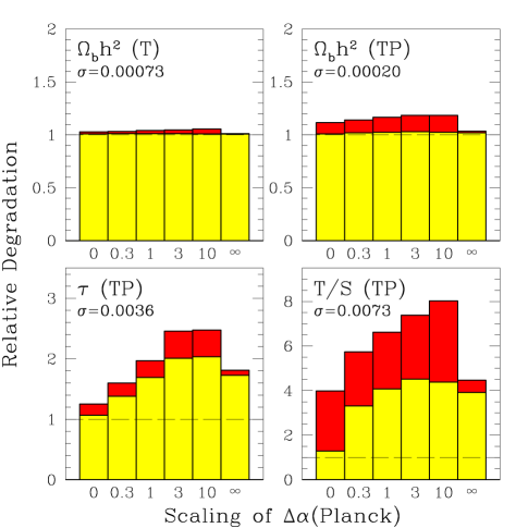
Adding and Removing Knowledge of Foregrounds
Boomerang MAP Planck Foreground Knowledge $\Omega_{b}h^{2}(T)$ $\Omega_{b}h^{2}(T)$ $\Omega_{b}h^{2}(TP)$ $\tau(TP)$ $T/S(TP)$ $\Omega_{b}h^{2}(T)$ $\Omega_{b}h^{2}(TP)$ $\tau(TP)$ $T/S(TP)$ Known Properties 1.000 1.000 1.000 1.000 1.000 1.000 1.000 1.000 1.000 Unknown $C_{\ell}$ 1.133 1.162 1.202 1.320 1.085 1.014 1.029 1.097 1.185 Unknown $\Theta$ 1.036 1.022 1.164 1.222 1.175 1.012 1.073 1.010 1.121 Unknown ${\bf R}$ 1.000 1.014 1.026 1.078 1.021 1.000 1.010 1.016 1.084 Unknown $\Theta$ & ${\bf R}$ 1.106 1.089 1.292 1.374 1.288 1.019 1.098 1.071 1.482 Unknown $C_{\ell}$ & ${\bf R}$ 1.151 1.230 1.376 1.458 1.227 1.014 1.049 1.109 1.290 Unknown $C_{\ell}$ & $\Theta$ 1.164 1.194 1.390 1.545 1.281 1.018 1.093 1.107 1.296 Unknown, except: Known Free-free 1.098 1.348 1.616 1.755 1.414 1.023 1.132 1.161 1.619 Known Synchrotron 1.140 1.387 1.622 1.622 1.378 1.024 1.117 1.115 1.411 Known Vibrating Dust 1.172 1.208 1.278 1.266 1.136 1.024 1.122 1.133 1.492 Known Rotating Dust 1.221 1.320 1.585 1.656 1.367 1.024 1.127 1.140 1.515 Known Thermal SZ 1.221 1.385 1.661 1.756 1.421 1.022 1.137 1.163 1.626 Known Radio PS 1.185 1.238 1.447 1.691 1.364 1.007 1.063 1.143 1.589 Known Infrared PS 1.209 1.218 1.411 1.671 1.348 1.022 1.107 1.097 1.535 All Unknown 1.221 1.415 1.674 1.756 1.424 1.024 1.137 1.163 1.626

NOTES.—Errors on cosmological parameters as we alter the knowledge of the foreground model. All numbers are listed relative to the results when the foreground properties are known; note that this differs from the convention of Table 3. All results use the MID foreground model. A prior of 10 has been used on the SZ component except where stated. In the first half of the table, we progressively introduce each of the three different types of variations, applying them to all of the foreground components. The sets of foreground parameters for the frequency dependence (${\mathbf{q}}_{(k)}^{P}$), the frequency coherence (${\mathbf{r}}_{(k)}^{P}$), and the shape of the spatial power spectrum (${\mathbf{s}}_{(k)}^{P}$) are denoted by $\Theta$, ${\bf R}$, and $C_{\ell}$, respectively. Note that the normalization of the fluctuations is carried by the $\Theta$ uncertainties. Higher errors indicate that the experiment’s performance is particularly sensitive to those uncertainties of the foregrounds. In the second half of the table, we consider all the foreground properties to be unknown except for those of a given component. Lower errors indicate that external information on that foreground would be particularly valuable.

5.4.4 Dependence on foreground type

We next consider the results when all foregrounds properties are unknown save for those of a single component. This can identify the component about which external information would have the most importance in improving cosmological inferences. The results are again shown in Table 4. For Boomerang, we find that uncertainties in the foregrounds are not contributing much additional degradation beyond the mere presence of the foregrounds; the largest remaining concern is that free-free or synchrotron emission might have a high-frequency contribution. For MAP, improving knowledge of the vibrating dust has the most impact, on both the large-angle polarization signals and the small-angle acoustic features. Better control of point sources would help $\Omega_{b}h^{2}$ from temperature information, but one should recall that our foreground model allows non-monotonic excursions in the power spectrum of the point sources and so may be overly pessimistic. Further, MAP suffers significant degradation unless the thermal SZ is controlled by an external prior of a factor of 10, so robust calculations of the power spectrum of this effect as a function of cosmology will be required. For Planck, no foreground makes an enormous difference by itself, although radio point sources have the largest (but still small) effect.

5.4.5 Dependence on polarization type

Figure 25.— Information about cosmological parameters from different polarization types. In each panel, the bars show the relative error bars using all information ($TXEB$), all but $B$-polarization ($TXE$), $T$ and $X$ only ($TX$), $T$ and $E$ only ($TE$) and unpolarized intensity alone ($T$). Results are shown both without any foregrounds (yellow) and for the MID foreground scenario with known properties (red). Note that these color conventions differ from those in Figure 19–24 and 26 and also that this figure uses a Gaussian rather than exponential coherence function. The rightmost bars in the $\tau$ panels extend far off the scale.

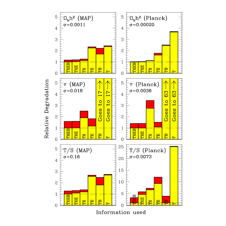
For which polarization type would prior knowledge of the foreground properties most help cosmological parameter estimation? The answer to this question depends on where the cosmological parameter information is coming from in the first place, and this in turn depends on the parameter in question. Limiting ourselves first to the case of known foreground properties, we can answer this question using equation (47). If foregrounds and/or systematic errors made the measured power spectrum $\tilde{C}_{\ell}^{P}$ completely unusable, this would correspond to adding in infinite amount of noise to the element ${\bf M}_{PP}$ of the $4\times 4$ covariance matrix of equation (45). The Fisher matrix ${\bf F}_{\ell}$ of equation (47) therefore gets replaced by

$${\bf F}^{\prime}_{\ell}\equiv\lim_{t\to\infty}\left[{\bf F}^{-1}_{\ell}+{\bf J}t\right]^{-1},$$ (63)

where the ${\bf J}$ is a $4\times 4$ matrix with zeroes everywhere except in element $(P,P)$; ${\bf J}_{P^{\prime}P^{\prime\prime}}\equiv\delta_{PP^{\prime}}\delta_{PP^{\prime\prime}}.$ This corresponds to simply crossing out row $P$ and column $P$ of ${\bf F}_{\ell}$, inverting the remaining $3\times 3$ matrix, and padding with zeroes. For example, if we drop the information from $X$-polarization, we obtain

$${\bf F}^{\prime}_{\ell} = 2\left(\hskip-5.69046pt\begin{tabular}[]{cc}$\>\left[\hskip-5.69046pt\begin{tabular}[]{ccc}$T_{\ell}^{2}$&$X_{\ell}^{2}$&$0$\\[2.0pt] $X_{\ell}^{2}$&$E_{\ell}^{2}$&$0$\\[2.0pt] $0$&$0$&$B_{\ell}^{2}$\end{tabular}\hskip-5.69046pt\right]^{-1}$&$\hskip-5.69046pt\begin{tabular}[]{ccc}$0$\\[2.0pt] $0$\\[2.0pt] $0$\end{tabular}\hskip-5.69046pt$\\ $\hskip-14.22636pt\begin{tabular}[]{c\skippp c\skippp c}$0$&$0$&$0$\end{tabular}\hskip-5.69046pt$&$0$\end{tabular}\hskip-5.69046pt\right)$$ (73)

$$= {2\over D_{\ell}^{2}}\left(\hskip-5.69046pt\begin{tabular}[]{cccc}$E_{\ell}^{2}$&$-X_{\ell}^{2}$&0&$0$\\[2.0pt] $-X_{\ell}^{2}$&$T_{\ell}^{2}$&0&$0$\\[2.0pt] $0$&$0$&$\displaystyle{D_{\ell}^{2}\over B_{\ell}^{2}}$&$0$\\[2.0pt] $0$&$0$&0&$0$\end{tabular}\hskip-5.69046pt\right),$$ (78)

where the notation is the same as in equation (46). Likewise, omitting two of the four power spectra corresponds to crossing out two rows and columns before inverting, etc., so we can compute the attainable accuracy on cosmological parameters using any subset of the four power spectra $T$, $E$, $B$ and $X$.

Figure 25 shows the results for our sample of three cosmological parameters using five such subsets. Comparing $T$ alone with the other cases illustrates the well-known fact that polarization helps substantially, especially with $\tau$ and $T/S$ (see e.g., Hogan et al. 1982; Bond & Efstathiou 1987; Zaldarriaga et al. 1997). We find that all parameters that are sensitive to the acoustic peaks are like $\Omega_{b}h^{2}$ in that the bulk of the polarization gain is coming from $X$-polarization, manifested by $T+X$ giving smaller error bars than $T+E$ and by the combination $T+X+E$ being only marginally better than $T+X$. On the other hand for $\tau$, $E$ is seen to be more important than $X$ for picking up the large-scale bump caused by early reionization. The $B$ channel receives contributions from gravity waves alone. However it dominates the measurement of $T/S$ only for Planck because MAP does not have enough signal-to-noise to yield interesting constraints on the $B$-polarization.

These results imply that a better understanding of foreground polarization in $X$ would most improve errors for $\Omega_{b}h^{2}$, $E$ for $\tau$ and ultimately $B$ for $T/S$. We also test these conclusions in the case of simultaneous estimation of foreground and cosmological parameters by placing priors separately on each of the polarization types; the results confirm these tendencies.

6. Conclusions

We have presented a comprehensive treatment of microwave foregrounds and the manner in which they degrade our ability to measure cosmological parameters with the CMB. Having developed three quantitative models, we compute their effect upon the Boomerang, MAP and Planck missions, including the level of foreground residuals in the cleaned maps for various scenarios and the extent to which this residual contamination would degrade the measurement of cosmological parameters. We consider both the case when the foreground power spectra are known and the case in which they must be computed from the CMB data itself. Our foreground model can be found at www.sns.ias.edu/$\sim$max/foregrounds.html together with software implementing our cleaning algorithm.

Our results are generally encouraging, in that the experiments perform well in the face of rather severe foreground models. This success derives from the fact that the cosmic signals can be distinguished from foregrounds by their frequency dependence, their frequency coherence, and their spatial power spectra. With these handles on the cosmic signal, we find that the error bars on most cosmological parameters are degraded by less than a factor of two for our best-guess foreground model and by less than a factor of five in our most pessimistic scenario. Effects producing large-angle polarization signals, namely reionization and tensor perturbations, suffer more because of their intrinsically small cosmic amplitude, but even these can be accurately extracted in most cases.

6.1. The most damaging foregrounds

One useful result of this work is that it highlights which foregrounds are potentially most damaging for precision cosmology and therefore most in need of further study. We find that allowing for uncertainties in the properties of the foregrounds does cause a substantial degradation in performance relative to the case of known foreground properties. In the study of the acoustic peaks, these uncertainties were dominant; however, in the study of large-angle polarization, the mere presence of sample variance from the foregrounds was more important for Planck.

Taken alone, the uncertainties in the shape of the power spectra were more important that the uncertainties in either the frequency dependence or the frequency coherence. In the case of tensors, the combination of frequency dependence and frequency coherence were particularly important. Of course, combinations of excursions are usually worse than the sum of individual excursions.

In the case of MAP, adding external information about vibrating dust made the most improvement in the results. Point source information also helped in the temperature data on the acoustic peaks. Knowing the level of thermal SZ fluctuations from filaments to within a factor of 10 a priori noticeable improved the results, so order-of-magnitude limits on this effect from simulations or observations will be valuable. In the case of Boomerang, restricting the ability of free-free and synchrotron emission to pollute the 90 GHz channel was most important. Clearly, MAP and Boomerang will complement each other in their constraints on possible pathologies of the intensity of foregrounds, as the experiments cover relatively low and high frequencies, respectively. In the case of Planck, the foreground cleaning in the MID model was sufficiently good that most foregrounds had only a minor impact. The largest degradations were due to radio point sources and synchrotron radiation.

Since we found that temperature-polarization cross-correlation carries much more information than $E$-polarization on most cosmological parameters (the exceptions being $\tau$ and $T/S$), it is clearly important to accurately model and measure the cross-correlation between polarized and $E$-unpolarized foregrounds.

6.2. Robustness

Figure 26.— As Figure 19, but showing the relative degradation in error bars from MAP on four cosmological parameters as the amplitude of foregrounds are increased. The histograms show results for a series of foreground models based on our MID model, with amplitudes of all components multiplied by 0 (i.e. no foregrounds), 1, 3, and 10. The results are scaled to the no-foreground case; the $1-\sigma$ errors in this case are listed in each panel. (lightly-shaded) Results with foregrounds of known properties. (heavily-shaded) Results with foregrounds with unknown parameters that must be simultaneously estimated from the CMB data.

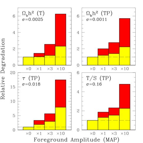
How robust are these results? Have we been to conservative or too optimistic? In general, we have tried to err on the side of caution, occasionally to the point of playing the role of the Devil’s advocate. We view the MID model as slightly cautious and the PESS model as quite extreme, on the verge of being ruled out by current constraints. We have also been conservative in not taking advantage of foreground dependence on Galactic latitude except in the crudest way, with a Galactic cut. In the same spirit, we have not included information from non-CMB templates such as the DIRBE or Haslam maps. The formalism we have presented is general enough that both of these types of additional information can be included, the latter simply by including the foreground templates as additional “channels” in the analysis.

However, there are also ways in which real-world foregrounds may be worse than we have assumed. We have made the simplifying assumption that each physical component is separable in $\ell$ and $\nu$, i.e., that only the amplitude (not the shape) of its power spectrum depends on frequency. This needs to be tested empirically, and may reveal that certain foregrounds decompose into several separable subcomponents. Perhaps most importantly, we have modeled foregrounds as Gaussian, which is certainly incorrect at some level. Our removal method still succeeds in minimizing the rms residual even if the foregrounds are non-Gaussian, and all our plots of residual power spectra remain correct (since they involve second moments only), but the error bars on the measured power spectra (which involve fourth moments) that propagate into the calculations of cosmological parameter accuracy will change in this case, probably for the worse. As mentioned, the variance of a measurement of say $C_{\ell}$ will be $2/N$ for the Gaussian case, where $N=(2\ell+1)f_{\rm sky}$ is the effective number of independent modes that probe this quantity. For a measurement of the band power between $\ell_{1}$ and $\ell_{2}$, we have $N=[(\ell_{2}+1)^{2}-\ell_{1}^{2}]f_{\rm sky}$ modes. Foreground non-Gaussianity typically correlates these modes, reducing the effective number of independent modes and thereby increasing the variance on the measured multipole or band power. We explore the effect of such errors in a very crude way in Figure 26, by simply increasing the foreground amplitudes by various factors $Q$. An amplitude increase $Q$ causes an increase in the power spectrum of $Q^{2}$, corresponding to a variance increase of $Q^{4}$ and a reduction of $N$ by $Q^{4}$. For instance, increasing all foreground amplitudes by a factor $Q=10$ corresponds to reducing the number of independent modes by 10,000. This is likely to be more severe than the actual level of foreground non-Gaussianity, since it would imply, e.g., that all 10,000 multipole modes $a_{\ell m}$ up to $\ell=100$ would be almost perfectly correlated. It should be noted that in the extreme case where non-Gaussianity gives perfect correlations between neighboring multipoles, foregrounds become trivial to remove by projecting out an overall offset. In other words, the worst possible case lies somewhere in between the extremes of no mode correlation and complete mode correlation. A detailed study of the non-Gaussian properties of foregrounds would certainly be worthwhile, using, e.g., the WOMBAT compilation of foreground data (Gawiser et al. 1999).

6.3. Comparison with other work

A number of excellent treatments of foregrounds and their impact on CMB measurements have been published. Thorough and recent ones that are particularly relevant to this paper are those done for the Planck proposal (TE96; Bouchet et al. 1996; Bersanelli et al. 1996; Bouchet et al. 1998; AAO 1998; BG99) and K99. Although these studies did not compute the accuracies with which cosmological parameter could be measured, they all calculated residual power spectra in the cleaned maps and their associated error bars, which can be compared with ours. We typically find slightly higher levels of residual foreground. Apart from minor differences in the assumed foreground power spectra etc, this is because we do not assume that the foreground covariance between different frequencies is a matrix of rank 1 or 2. The former assumption (made in, e.g., TE96 and Bersanelli et al. 1996) corresponds to assuming $\Delta\alpha=0$, i.e., perfect frequency coherence. The latter, used in for instance BG99 and K99, is equivalent to assuming that each foreground can be decomposed into two perfectly coherent components.

The elegant treatment of K99 gives foregrounds even more leeway than we have, with thousands of free parameters, allowing their power spectra to be completely arbitrary functions of $\ell$ and fitting for them directly from the data. Unfortunately, this only works for the above-mentioned rank 2 assumption about coherence for Planck, since the number of components cannot exceed half of the number of channels. We have restricted the foreground power spectra, frequency spectra and frequency correlations to be fairly smooth functions, since all such functions measured to date have been fairly dull and featureless.

6.4. Outlook

A large number of papers have now painted a rosy picture of the future of cosmology, with CMB experiments measuring cosmological parameters to unprecedented accuracy over the next decade. In this paper, we have tried quite hard to spoil this picture, using foreground models with hundreds of harmful parameters and pushing them to limits of physical plausibility and current constraints. Although we have found that great care needs to be taken in the foreground removal phase of the data analysis to avoid potentially perilous pitfalls, we have failed to tarnish the overall picture with more than a few minor blemishes, degrading the accuracy on certain measurements by small factors. Although much work certainly remains to be done on the foreground problem, this is cause for cautious optimism.

Acknowledgements: We thank John Bahcall, Lloyd Knox, David Spergel, Alexei Tchepurnov, Philip Tegmark, Matias Zaldarriaga and an anonymous referee for helpful comments, Luigi Toffolatti for kindly providing his source count model data, and Uroš Seljak & Matias Zaldarriaga for their CMBFAST code, which was used for generating our CMB power spectra. We thank the Alfred P. Sloan Foundation for funding the foreground workshop where this work was first presented, and the workshop participants for useful comments and suggestions. This work was supported by NASA though grant NAG5-6034 and Hubble Fellowship HF-01084.01-96A from STScI, operated by AURA, Inc. under NASA contract NAS5-26555. D.J.E. is supported by a Frank and Peggy Taplin Membership at the IAS, W.H. by the W.M. Keck Foundation, and D.J.E. and W.H. by NSF-9513835.

REFERENCES

AAO for Planck HFI and LFI proposals submitted in response to the Announcement of Opportunity of ESA, 1998

Aghanim, N., de Luca, A., Bouchet, F. R., Gispert, R., & Puget, J. L. 1997, A&A, 325, 9

Banday, A. J., & Wolfendale, A. W. 1991, MNRAS, 248, 705

Bersanelli, M. et al. 1996, COBRAS/SAMBA, Phase A Study for an ESA M3 Mission, ESA Report D/SCI(96)3, http://astro.estec.esa. nl/SA-general/Projects/Planck/report/report.html

Bennett, C. L et al. 1992, ApJL, 396, L7

Bennett, C. L et al. 1994, ApJ, 436, 423

Bond, J. R., & Efstathiou, G. 1987, MNRAS, 227, 33P

Bond, J. R., Efstathiou, G., & Tegmark, M. 1997, MNRAS, 291, L33

Bond, J. R., Jaffe, A. H., & Knox, L. 1998, astro-ph/9808264

Bouchet, F. R. et al. 1995, Space Science Rev., 74, 37

Bouchet, F. R., & Gispert, R. 1999, astro-ph/9903176 (“BG99”)

Bouchet, F. R., Gispert, R., & Puget, J. L. 1996, in Unveiling the Cosmic Infrared Background, ed. E. Dwek (AIP: Baltimore)

Bouchet, F. R., Prunet, S., & Sethi, S. K. 1999, MNRAS, 302, 663

Boughn, S. P., & Crittenden, R. G 1999, in Microwave Foregrounds, ed. A. de Oliveira-Costa & M. Tegmark (ASP: San Francisco)

Brandt, W. N. et al. 1994, ApJ, 424, 1

Brouw, W. N., & Spoelstra, T. A. T. 1976, A&AS, 26, 129

Cayón, L., Sanz, J. L., Argüeso, F., Martínez-González, E., & Barreiro, R. B. 1999, in Microwave Foregrounds, ed. A. de Oliveira-Costa & M. Tegmark (ASP: San Francisco)

Coble, K. et al. 1999, astro-ph/9902195

Cress, C. M., Helfand, D. J., Becker, R. H., Gregg, M. D., & White, R. L. 1996, ApJ, 473, 7

Davies, R. D., & Wilkinson, A. 1999, in Microwave Foregrounds, ed. A. de Oliveira-Costa & M. Tegmark (ASP: San Francisco)

de Luca, A., Désert, F. X., & Puget, J. L. 1995, A&A, 300, 335

de Oliveira-Costa, A., Kogut, A., Devlin, M. J., Netterfield, C. B., Page, L. A., Wollack, E. J. 1997, ApJ, 482, L17

de Oliveira-Costa, A., Tegmark, M., Page, L. A., Boughn, S. 1998, ApJ, 509, L9

de Oliveira-Costa, A., Tegmark, M., Efstathiou, G., McKee, C., & Smoot, G. F. 1999b, in preparation

de Oliveira-Costa A, Tegmark, M., Jones, A. W., Gutierrez, C. M., Davies, R. D., Lasenby, A. N., Rebolo, R., & Watson, R. A. 1999a, astro-ph/9904296

de Zotti, G., Toffolatti, L., Argüeso,, .Davies, R. D., Mazzotta, P., Partridge, R. B., Smoot, G. F., & Vittorio, N. 1999, astro-ph/9902103

Dodelson, S. 1996, ApJ, 482, 577

Dodelson, S., & Jubas, J. M. 1995, ApJ, 439, 503

Dodelson, S., & Stebbins A 1994, ApJ, 433, 440

Draine, B. T., & Lazarian A 1998, ApJ, 494, L19 (“DL98”)

Draine, B. T., & Lazarian A 1999, astro-ph/9902356, in Microwave Foregrounds, ed. A. de Oliveira-Costa & M. Tegmark (ASP: San Francisco)

Duncan, A. R., Haynes, R. F., Jones, K. L., & Stewart, R. T. 1997, MNRAS, 291, 279

Duncan, A. R., Haynes, R. F., Jones, K. L., & Stewart, R. T. 1998, MNRAS, 291, 279

Eisenstein, D. J., Hu, W., & Tegmark M 1999, astro-ph/9807130

Ferreira, P. G., & Magueijo, J. 1997, Phys. Rev. D, 55, 3358

Finkbeiner, D. P. et al. 1999, in preparation

Finkbeiner, D. P., & Schlegel, D. J. 1999, in Microwave Foregrounds, ed. A. de Oliveira-Costa & M. Tegmark (ASP: San Francisco)

Franceschini, A. et al. 1989, ApJ, 344, 35

Gautier, T. N. I., Boulanger, M., Perault, M., & Puget, J. L. 1992, AJ, 103, 1313

Gawiser, E., Jaffe, A. & Silk J 1998, astro-ph/9811148

Goldberg, D. M., & Spergel, D. N. 1999, astro-ph/9811251

Guarini, G., Melchiorri, B., & Melchiorri, F. 1995, ApJ, 442, 23

Guiderdoni, B. 1999, astro-ph/9903112, in Microwave Foregrounds, ed. A. de Oliveira-Costa & M. Tegmark (ASP: San Francisco)

Guiderdoni, B., Hivon, E., Bouchet, F. R., & Maffei, B. 1998, MNRAS, 295, 877

Gutierrez, C. M.,Rebolo, R., Watson, R. A., Davies, R. D., Jones, A. W., & Lasenby, A. N. 1999, astro-ph/9903196

Haiman, Z., & Knox, L. 1999, astro-ph/9902311, in Microwave Foregrounds, ed. A. de Oliveira-Costa & M. Tegmark (ASP: San Francisco)

Hobson, M. P., Jones, A. W., Lasenby, A. N., & Bouchet, F. R. 1998, astro-ph/9806387

Hogan, C. J., Kaiser, N., & Rees, M. J. 1982, Phil. Trans. R. Soc. Lond., A307, 97

Holder, G. P., & Carlstrom, J. E. 1999, in Microwave Foregrounds, ed. A. de Oliveira-Costa & M. Tegmark (ASP: San Francisco)

Hu, W., Scott, D., & Silk, J. 1994, Phys. Rev. D, 49, 648

Hu, W., & Sugiyama, N. 1995, ApJ, 444, 489

Hu, W., & White, M. 1996, A&A, 315, 33

Hu, W., & White, M. 1997, New Astron, 2, 323

Jaffe, A. H. et al. 1999, astro-ph/9903248, in Microwave Foregrounds, ed. A. de Oliveira-Costa & M. Tegmark (ASP: San Francisco)

Jewell, J. 1999, astro-ph/9903201, in Microwave Foregrounds, ed. A. de Oliveira-Costa & M. Tegmark (ASP: San Francisco)

Jonas, J. L. 1999, Ph.D. thesis, Rhodes University, South Africa

Jones, A. W. 1999, astro-ph/9905087, in Microwave Foregrounds, ed. A. de Oliveira-Costa & M. Tegmark (ASP: San Francisco)

Kamionkowski, M., Kosowski, A., & Stebbins, A. 1997, Phys. Rev. D, 55, 7368

Lue, A., Wang, L., & Kamionkowski, M. 1999, astro-ph/9812088

Keating, B., Timbie, P., Polnarev A, & Steinberger J 1998, ApJ, 495, 580

Kendall, M. G., & Stuart, A. 1969, The Advanced Theory of Statistics, Vol. II (Griffin: London)

Knox, L. 1995, Phys. Rev. D, 48, 3502

Knox, L. 1999, astro-ph/9811358

Kogut, A. 1999, in Microwave Foregrounds, ed. A. de Oliveira-Costa & M. Tegmark (ASP: San Francisco)

Kogut, A. et al. 1996, ApJL, 464, L5 (“K96”)

Leitch, E. M., Readhead, A. C. S., Pearson, T. J., & Myers, S. T. 1997, ApJ, 486, L23

Lim, M. A. 1996, ApJ, 469, 69L

Low, F. J., & Cutri, R. M. 1994, Infrared Phys. & Technol., 35, 291

Lubin, P., & Smoot, G. F. 1991, ApJ, 245, 1

Mann, R. G. 1999, astro-ph/9902340, in Microwave Foregrounds, ed. A. de Oliveira-Costa & M. Tegmark (ASP: San Francisco)

McCullough, P. R., Gaustad, J. E., Rosing W, & van Buren D 1999, astro-ph/9902248, in Microwave Foregrounds, ed. A. de Oliveira-Costa & M. Tegmark (ASP: San Francisco)

Ostriker, J. P., & Vishniac, E. 1.986, ApJ, 306, 51

Persi, F. M., Cen, R., & Ostriker, J. P. 1995, ApJ, 442, 1

Platania, P. et al. 1998, ApJ, 505, 473

Prunet, S., Sethi, S. K., & Bouchet, F. R. 1998a, astro-ph/9803160

Prunet, S., Bouchet, F. R., & Sethi, S. K., 1998b, submitted

Prunet, S., & Lazarian A 1999, in Microwave Foregrounds, ed. A. de Oliveira-Costa & M. Tegmark (ASP: San Francisco)

Reach, W. T. et al. 1995, ApJ, 451, 188

Refregier A, Spergel, D. N., & Herbig, T. 1998, astro-ph/9806349

Refregier, A. 1999, in Microwave Foregrounds, ed. A. de Oliveira-Costa & M. Tegmark (ASP: San Francisco)

Rephaeli, Y. 1995, ARA& A, 33, 541

Rybicki, G. B., & Lightman, A. 1979, Radiative Processes in Astrophysics (Wiley & Sons: New York)

Sachs, R. K., & Wolfe, A. M. 1967, ApJ, 147, 73

Schlegel, D. J., Finkbeiner, D. P., & Davis, M. 1998, ApJ, 500, 525

Scott, D., Srednicki, M., & White, M. 1994, ApJL, 421, L5

Scott, D. , & White, M. 1999, A&A, 346, 1

Smoot, G. F. 1999, astro-ph/9902201, in Microwave Foregrounds, ed. A. de Oliveira-Costa & M. Tegmark (ASP: San Francisco)

Staggs, S. T., Gundersen, J. O., & Church, S. E. 1999, astro-ph/9904062, in Microwave Foregrounds, ed. A. de Oliveira-Costa & M. Tegmark (ASP: San Francisco)

Stebbins, A. 1997, astro-ph/9709065

Sunyaev, R. A., & Zel’dovich, Y. 1970, Astroph. Sp. Sci., 7, 3

Tchepurnov, A. V. 1997, Nizhnij Arkhyz preprint 122

Tegmark, M. 1997a, ApJ, 480, L87

Tegmark, M. 1997b, Phys. Rev. D, 56, 4514

Tegmark, M., Taylor, A. N., & Heavens, A. F. 1997, ApJ, 480, 22

Tegmark, M. 1998, ApJ, 502, 1 (“T98”)

Tegmark, M., & de Oliveira-Costa, A. 1998, ApJ, 500, 83

Tegmark, M., de Oliveira-Costa, A., Devlin, M. J., Netterfield, C. B., Page, L., & Wollack E J 1996, ApJL, 474, L77

Tegmark, M., & Efstathiou, G. 1996, MNRAS, 281, 1297 (“TE96”)

Tegmark, M., & Villumsen, J. V. 1996, MNRAS, 289, 169

Tenorio, L., Jaffe, A. H., Hanany, S., & Lineweaver, C. H. 1999, astro-ph/9903206

Toffolatti, M. et al. 1998, MNRAS, 297, 117

Toffolatti, L., de Zotti, G., Argüeso, F., & Burigana C 1999, astro-ph/9902343, in Microwave Foregrounds, ed. A. de Oliveira-Costa & M. Tegmark (ASP: San Francisco)

Vishniac, E. 1987, ApJ, 322, 597

White, M. 1998, Phys. Rev. D, 57, 5273

Wright, E. L. 1979, ApJ, 232, 348

Wright, E. L. 1987, ApJ, 320, 818

Wright, E. L. 1996, astro-ph/9612006

Wright, E. L. 1998, ApJ, 496, 1

Zaldarriaga, M. 1998, ApJ, 503, 1

Zaldarriaga, M., & Seljak, U. 1999, astro-ph/9810257

Zaldarriaga, M., & Seljak, U. 1997, Phys. Rev. D, 55, 1830

Zaldarriaga, M., Spergel, D. N., & Seljak, U. 1997, ApJ, 488, 1

This paper is available with figures and fortran code from h t t p://www.sns.ias.edu/$\tilde{~{}}$max/foregrounds.html