Modeling Variable Emission Lines in AGNs:
Method and Application to NGC 5548

Abstract

We present a new scheme for modeling the broad line region in active galactic nuclei (AGNs). It involves photoionization calculations of a large number of clouds, in several pre-determined geometries, and a comparison of the calculated line intensities with observed emission line light curves. Fitting several observed light curves simultaneously provides strong constraints on model parameters such as the run of density and column density across the nucleus, the shape of the ionizing continuum, and the radial distribution of the emission line clouds.

When applying the model to the Seyfert 1 galaxy NGC 5548, we were able to reconstruct the light curves of four ultraviolet emission-lines, in time and in absolute flux. This has not been achieved by any previous work. We argue that the Balmer lines light curves, and possibly also the Mg ii $\lambda$2798 light curve, cannot be tested in this scheme because of the limitations of present-day photoionization codes. Our fit procedure can be used to rule out models where the particle density scales as $r^{-2}$, where $r$ is the distance from the central source. The best models are those where the density scales as $r^{-1}$ or $r^{-1.5}$. We can place a lower limit on the column density at a distance of 1 ld, of $N_{col}(r=1)\mathrel{\raise 1.29167pt\hbox{$>$}\mkern-14.0mu\lower 2.58334pt\hbox{$\sim$}}10^{23}$ cm^-2 and limit the particle density to be in the range of $10^{12.5}>N(r=1)>10^{11}$ cm^-3.

We have also tested the idea that the spectral energy distribution (SED) of the ionizing continuum is changing with continuum luminosity. None of the variable-shape SED tried resulted in real improvement over a constant SED case although models with harder continuum during phases of higher luminosity seem to fit better the observed spectrum. Reddening and/or different composition seem to play a minor role, at least to the extent tested in this work.

1. Introduction

Broad emission-Line Regions (BLRs) in Active Galactic Nuclei (AGNs) have been the subject of extensive studies for more than two decades. These regions are not spatially resolved and information about their size, and the gas distribution, can only be obtained via reverberation mapping. Understanding such regions requires a combination of detailed observations with sophisticated theoretical models.

The extensive monitoring campaigns, of the last decade, focused on the broad line emission, variability, and response of the broad emission lines to the continuum variations in more than a dozen AGNs (see Peterson 1993 and Netzer & Peterson 1997, for reviews). A major result is that in all well studied cases, the BLR is stratified with a typical size of order of light weeks in Seyfert galaxies and light months in quasars. Present day modeling of such stratified BLRs leaves much to be desired. While time-averaged spectra of AGNs can reasonably be explained by photoionization models (Netzer 1990 and references therein), there is a lack of detailed models fitting to the actual gas distribution, and motion, as deduced from the reverberation studies.

This paper investigates the physical conditions in the line emitting gas of a well studied AGN by incorporating modern photoionization calculations into a detailed geometrical model. Our approach, that requires the simultaneous fit of several emission line light curves, enables us to constraint several important properties of the BLR, such as the gas density, column density and level of ionization. The model is rather complex and is, therefore, limited to a spherical BLR with no attempt to reconstruct the velocity field. In § 2 we present the model, in § 3 we apply it to the Seyfert 1 galaxy NGC 5548, and in § 4 we discuss the new results in view of past studies.

2. The Model

2.1. Motivation, choice of target and previous work

Years of intensive AGN monitoring resulted in a wealth of information on the BLR response to continuum variations. Excellent data sets are now available for half a dozen sources and less complete sets on a dozen or so more. Unfortunately, theoretical understanding lags behind and there are few, if any, systematic attempts to produce complete models for the objects in questions. Most theoretical efforts have been limited to modeling of only one or two emission lines. They did not consider real limitations such as the gas density and column density. Our goal is to reconstruct all the observed light curves. This will enable us to set stringent limits on the physical parameters of the gas. More specifically, the aim is to deduce the run of density, column density and cloud distribution across the BLR. We will demonstrate that the time dependent relative and absolute line intensities, and their relationship to the continuum fluctuations, leave little freedom in such models. In particular, the density and column density are restricted to a rather limited range.

We wish to use as many observational constraints as possible and, therefore, limit ourselves to the best available data sets. We need both recombination lines, to constraint the covering factor, and collisionally excited lines to set limits on the run of density and temperature. Data sets including both high and low ionization lines are preferred since, in this way, we can set limits on the run of ionization parameter as a function of distance from the continuum source. Most importantly, we chose to rely as little as possible on Balmer line intensities since, as explained below, their calculated intensities are subjected to large theoretical uncertainties. Thus, the chosen data set must include a large enough number of UV lines and a well sampled, preferably large amplitude variable continuum. The only information that will not be used in this work is line profiles.

Given the above limitations, there are only 4 data sets that we consider suitable: 1. NGC 4151 - see Crenshaw et al. (1996) and references therein 2. NGC 5548 (Clavel et al. 1991) 3. NGC 3783 (Reichert et al. 1994) 4. NGC 7469 (Wanders et al. 1997). Out of those we chose to model the 1989 UV data of NGC 5548. This data set is unique in terms of its relatively large line and continuum variations, the combination of long duration with intensive regular 4-day sampling, and complete information on all strong UV lines (see however comments about Mg ii $\lambda$2798 in the discussion section). Other advantages of this light curve are discussed below.

In modeling the gas distribution in the nucleus, we distinguish between direct and indirect methods. Direct methods are those where one guesses a gas distribution and calculates the resulting line light curves by putting, through this geometry, the observed (or deduced) continuum light curve. The result is compared with the observed emission-line light curves. Indirect methods attempt to obtain the gas distribution by computing transfer functions. This procedure is somewhat ill-defined since it produces responsivity maps, rather than mass-distribution maps. It therefore requires the additional confirmation that the so-obtained responsivity maps are consistent with photoionization calculations. There have been several attempts to produce transfer functions for various lines in NGC 5548, we are not aware of any successful mapping that is consistent with full photoionization calculations (see also Maoz 1994).

Several previous attempts to model the BLR in NGC 5548 differ from the present study in several important ways. The first systematic attempt to reconstruct the BLR is by Krolik et al. (1991). These authors used photoionization calculations to find the parameters that best fit the mean observed line rations. In parallel, they have used the Maximum Entropy Method to reconstruct several transfer functions. Based on these transfer functions, they modeled a spherically symmetric BLR with locally isotropic line emitting clouds. The BLR is divided into two distinct zones: one emitting the high-ionization lines (column density of $\sim 10^{22}$ cm^-2 and ionization parameter of 0.3) and the other emitting the low-ionization lines (column density of $\sim 10^{23}$ cm^-2 and ionization parameter of 0.1).

O’Brien, Goad, & Gondhalekar (1994) have combined photoionization and reverberation-mapping calculations in a way similar to the present study (§ 2.2). Their work, and also the one by Pérez, Robinson & de la Funte (1992), focused on the shape of the transfer function and the line responsivity in a few generic models. They did not attempt a detailed reconstruction of a specific data set, and the comparison with the observations includes only time lags, and not the detailed shape of the light curves.

Shields, Ferland, & Peterson (1995) used photoionization calculations to examine the C iv $\lambda$1549/Ly$\alpha$ line ratio in NGC 5548 and other objects. They concluded that an optically thin non-variable component contributes to the BLR high ionization lines. Bottorff et al. (1997) presented a detailed kinematic model which they combined with photoionization calculations. They applied this model to one emission line (C iv $\lambda$1549) in the spectrum of NGC 5548.

Dumont, Collin-Suffrin, & Nazarova, (1998) modeled the BLR in NGC 5548 as a 3-zone region where the location of the various components were determined by the mean line-to-continuum lags. These authors assumed high column density ($\geq 10^{23}$ cm^-2) and photon density (the ionization parameter multiplied by the hydrogen density gives 10⁹ to 10¹⁰ cm^-3). Much of their conclusion regarding the density and column density is based on the relative strength of the Balmer lines which we consider to be unreliable for reasons we describe below. Like most others, they did not compare the observed shape of the emission line light curves with the prediction of the model.

Finally, in a recent work, Goad and Koratkar (1998) re-examined the 1989 NGC 5548 data set and deduced a strong radial dependence for the gas density ($N\propto r^{-2}$, with density in the range of 10${}^{11.3}-10^{10.0}$ cm^-3). Here again, the main assumption is of a two-zone model and there is no attempt to use the observed light curves, only the measured time lags.

Evidently, there is a definite lack of modeling complete data sets, i.e. the information provided by half a dozen emission line light curves. The published works focus on either detailed photoionization calculations or detailed geometrical modeling (i.e. using transfer functions) and no study have combined the two in a satisfactory way. Thus, no previous work has demonstrated that the assumed gas distribution, and the calculated physical conditions, are indeed compatible. Global consistency checks are certainly required.

Our work relies heavily on the direct approach. We prefer to avoid, as much as possible, ill-defined transfer functions and unreliable mass distributions. Instead we make a large number of initial assumptions (“guesses”) and check them, one by one, against the complete data set of NGC 5548. This makes the numerical procedure more time-consuming but is more robust because of the direct relationship between the assumed geometry and the resulting light-curves. It also allow us to assess, in a more meaningful way, the statistical significance of our results.

2.2. Formalism

We follow the approach described by Netzer (1990) for a BLR consisting of numerous small clouds and a point-like ionizing source. The contribution of each cloud to the various emission lines is determined by the physical conditions within the cloud and its distance from the center. The main assumption is that the cloud pressure is controlled by an external medium (magnetic field, hot gas, etc.) whose pressure is a simple function of the radius, $P\propto r^{-s}$. For completeness, we summarize below the main ingredients of the model.

Consider a spherical system of clouds around a central radiation source and assume pure radial dependence of all properties. The hydrogen number density, $N(r)$, assumed to be constant within each cloud, is controlled by equilibrium with the external pressure. Neglecting the small electron temperature variation we take this to be

$$N(r)\propto r^{-s}\ \ .$$ (1)

Next, we define the cloud column density, $N_{col}$, by considering spherical clouds, of radius $R_{c}(r)$. The mass of the individual clouds is conserved, as they move in or out, but it is not necessarily the same for all clouds, thus, $R_{c}^{3}(r)N(r)=const$. The cloud mean (over the sphere) column density is thus

$$N_{col}(r)\propto R_{c}(r)N(r)\propto r^{-2/3s}\ \ ,$$ (2)

and the geometrical cross-section is

$$A_{c}(r)\propto R_{c}^{2}(r)\propto r^{2/3s}\ \ .$$ (3)

(Note that the mass conservation assumption is only essential if we are to avoid an additional free parameter that specifies the run of $N_{col}$ with distance). Finally, the number of clouds per unit volume is

$$n_{c}(r)\propto r^{-p}\ \ .$$ (4)

In the numerical integration we consider only one type of clouds (i.e. same size at the same $r$ for all clouds). Simple generalization of this scheme can involve a local population of clouds having some size distribution and the same $p$ for all sub-classes. This requires extra normalization (see below) which we decided to avoid at this stage.

The clouds are illuminated by a central source whose ionizing luminosity, $L(t)$, varies in time. Designating $\epsilon_{l}(r,L)$ as the flux emitted by the cloud in a certain emission-line, $l$, per unit projected surface area ($erg\ s^{-1}\ cm^{-2}$), we get the following relation for the emission of a single cloud:

$$j_{c,l}(r,L)=A_{c}(r)\epsilon_{l}(r,L)\ \ .$$ (5)

(where we note that in the actual calculations, we use a thin slab geometry, hence the geometrical cross section is somewhat different from $\pi R_{c}^{2}$). Assuming the system of clouds extends from $r_{in}$ to $r_{out}$ we obtain cumulative line fluxes:

$$E_{l}\propto\int_{r_{in}}^{r_{out}}n_{c}(r)j_{c,l}(r,L)r^{2}dr\ \ .$$ (6)

Having determined the properties of the emission line clouds, and having assumed a spectral energy distribution (SED) for the ionizing source, we now calculate $\epsilon_{l}(r,L)$ using a photoionization code. We then follow the above formalism to obtain $E_{l}$. Since all parameters have been fixed, there is no need to independently specify the ionization parameter, $U(r)$ which, in our model, is given by

$$U(r)=\frac{Q}{4\pi r^{2}N(r)c}\propto r^{s-2}$$ (7)

where Q is the number of hydrogen ionizing photons per second, and $c$ is the speed of light.

AGN emission is variable, causing the local emission-line flux to be a function of time. We take this into account by calculating $\epsilon_{l}(r,L(t))$ for the entire range of continuum luminosity applicable to the source under discussion. The calculated in situ line fluxes are, therefore, the result of integrating Eq. 6, using, at each distance $r$ the ionizing flux obtained with the ionizing luminosity $L(t-r/c)$. Observed fluxes further require the accounting for the light travel time between the cloud and the observer.

A model is specified by the source luminosity and SED, the radial parameter $s$, and the normalization of the various free parameters. These include $r_{in},\ r_{out}$ and the density and column density at a fiducial distance which we take to be one light-day (1 ld), i.e. outside the range of interest (in all the cases presented here $r_{in}>1$ ld). The comparison with observations further requires the normalization of the total line fluxes and hence the integrated number of clouds. We prefer to use the total covering factor $C(r_{out})$ which is obtained by integrating

$$dC(r)=A_{c}(r)n_{c}(r)dr\propto r^{2/3s-p}dr\ \$$ (8)

between $r_{in}$ and $r_{out}$. The normalization of $C(r_{out})$ is achieved by comparing the observed and calculated flux of the emission lines. The numbers quoted below refer to the total covering factor as determined by taking the mean covering factor derived for the individual lines. We do not consider cloud obscuration and the calculations are limited to values of $C(r_{out})$ smaller than about 0.3. Considering all this, the total number of free parameters in the model is seven.

Computing a single model is not a trivial task. The reason is that, as explained, $\epsilon_{l}(r,L(t))$ is a function of both distance and time. We have accomplished this by calculating large grids of photoionization models covering the required range of density, column density, and incident flux. The calculations were performed using ION97, the 1997 version of the code ION (see Netzer 1996, and references therein). The code includes a large number of atomic transitions and solves for the level of ionization, and the gas temperature, at each location, taking into account all optical depth effects. The line and continuum transfer is calculated by using the local escape probability formalism. The cloud geometry assumed is of a thin shell. This is somewhat different from the spherical-cloud assumption made here, but the uncertainty introduced is well below the uncertainty of the escape probability method.

A serious problem in ION, and in similar codes like Cloudy by G. Ferland (Ferland et al. 1998), is the treatment of the optically thick Balmer lines. The local escape probability approximation used in such codes is inadequate for these lines (Netzer 1990). Unfortunately, there is no known cure for this problem within that formalism and we have decided, therefore, not to consider Blamer lines in this work. The calculated intensity of other optically thick lines produced in the large, extended, low ionization zone of the cloud (e.g., Mg ii $\lambda$2798 and many FeII lines) is also considered uncertain. A further limitation is the anisotropy of line emission which can be important when emission line light-curves are concerned (see Ferland et al. 1992 and references therein). We have decided not to include this effect since the local escape probability method cannot accurately take it into account and since it depends on the cloud shape, which is unknown. We caution that while codes like ION and Cloudy calculate this anisotropy as part of their standard output, the fundamental limitation of the local escape probability method makes such numbers highly uncertain.

We have adopted a goodness of fit criteria to evaluate the model results. This is based on a simple $\chi^{2}$ score which is evaluated by comparing the observed and theoretical light cures of all chosen emission lines, giving each line an equal weight. Thus, an acceptable model must reproduce the correct line variability as well as the observed line ratios. To the best of our knowledge, no previous AGN model have posed such stringent conditions on the goodness of fit.

3. Modeling the BLR in NGC 5548

The Seyfert 1 galaxy NGC 5548 is a subject of an intensive study for more then a decade now. This includes optical spectroscopic monitoring for 8 years (Peterson et al. 1999, and references therein), several satellite monitoring campaigns in different wavelengths — each with a duration of several months (e.g., Nandra et al. 1993, Korista et al. 1995, Tagliaferri et al. 1996, Marshal et al. 1997), and many complementary studies of those data sets (e.g., Clavel et al. 1992, Maoz et al. 1993, Wanders & Peterson 1996). This, together with the reasons mentioned in § 2.1, makes NGC 5548 the best object for testing our model. In this study we have concentrated on the 1989 $International\ Ultraviolet\ Explorer\ (IUE)$ campaign (Clavel et al. 1991) and used the $\lambda$1337 continuum and five emission lines; Ly$\alpha\lambda$1216, C iv $\lambda$1549, C iii ] $\lambda$1909, He ii $\lambda$1640, and Mg ii $\lambda$2798.

On top of the general considerations described in the previous section, there are several constraints pertaining to NGC 5548:

1. The 1989 $IUE$ spectra, and the following HST observations (Korista et al. 1995), clearly show that the C iii ] $\lambda$1909 line is blended with Si iii ] $\lambda$1895. Clavel et al. (1991) have measured the combined flux of both lines, without deblending (this is the flux listed in their tables under the C iii ] $\lambda$1909 header). This is also the case in the Korista et al. (1995) paper. The observed ratio of C iii ] $\lambda$1909 to Si iii ] $\lambda$1895 in the mean spectrum of NGC 5548, is about 3:1. The line ratio, which is density dependent, provides an important constraint on the density. We calculate the intensities of the silicon and carbon lines and restrict ourselves to those models producing a ratio consistent with the observations. The diagrams and tables below gives the summed intensity under the title C iii ] $\lambda$1909.

2. Galactic and intrinsic reddening can affect the observed line ratios and the assumed ionizing continuum. We address this in § 3.4.

3. Another important consideration is the shape of the ionizing continuum. The observed SED of NGC 5548 is reviewed by Dumont et al. (1998) who discuss also various SEDs assumed in previous works. We have chosen a range of possible SEDs, all in agreement with observations of typical Seyfert 1 galaxies. Our optical-UV continuum is combined with the observed ASCA continuum of the source assuming $\alpha_{ox}$=1.06 (see George et al. 1998 for a discussion of the X-ray spectrum of NGC 5548). We have varied the assumed SED, as described in § 3.5, and tested the effect on the emission line spectrum. All chosen SEDs are rather similar to the ones discussed in Dumont et al. (1998). Our fiducial case is presented in Fig. 1 on the same scale as in Dumont et al. (1998).

4. Using the observed $\lambda$1337 continuum flux, a chosen cosmology ($H_{0}$=$75$ km s^-1Mpc^-1 and $q_{0}=0.5$), and the assumed SED, we have estimated the time averaged ionizing luminosity of NGC 5548 to be $\sim 10^{44}$ erg s^-1. The continuum flux at $\lambda$1337 varied by a factor of $\sim 4.5$, during the $IUE$ campaign. Hence we choose our grid to cover the ionizing luminosity range of $10^{43.6}$ to $10^{44.3}$ erg s^-1, with a step size corresponding to 0.1 in $\log{L}$. The observed $\lambda$1337 light curve was transformed into ionizing-luminosity light curve covering the entire range between these values - see Fig. 2. Considering the BLR geometry, we have defined our grid of distances to cover the range of 1 to 100 lds, with a step size of 0.02 in $\log{r}$.

5. We have adopted solar abundances for our standard model (see also § 3.2 below).

Model calculation proceed in two stages. First we produce two-dimensional grids of $\epsilon_{l}(r,L(t))$ by calculating, for each radial distance, all line emissivities for all ionizing luminosities. Each grid represents a particular choice of the density parameter $s$, and the density and column density at the fiducial distance. We consider three density laws: $s=1$, 1.5, and 2, a density at 1 ld of $\sim 10^{11}$ to $\sim 10^{13}$ (varying by a factor of $\sim$2 from one grid to the next) and column densities at 1 ld of $10^{22}$, $10^{23}$, and $10^{24}$. The choice of density, column density, $s$ and the time-variable luminosity, completely specify the ionization parameter at each location.

In the second stage we calculate theoretical light curves by integrating Eq. 6. For this we need to define $p$, $r_{in}$ and $r_{out}$. We have considered models with $p=1$, 1.5 and 2. For each of these we have varied $r_{in}$ and $r_{out}$ in order to minimize the calculated $\chi^{2}$.

An important consideration is the error bar size for the first few points. Obviously, we have no knowledge of the continuum behavior prior to the beginning of the campaign. We have therefore decided to extrapolated the continuum light curve, at a constant level, for all JD $<$ 2447510. This lack of knowledge introduces a large uncertainty in the first part of the line light-curves which is likely to be much larger than the pure observational error. To partly cure this effect, we have artificially increased all experimental error bars during the first 100 days. We used a multiplication correction factor which is 3.0 for day 1 and decreases linearly with time, to 1.0, on day 100 (JD=2447600).

3.1. A detailed example, $s=2$ models

To illustrate our method, we present the results of a model with $s=2$ (i.e. $N(r)\propto r^{-2}$ and $N_{col}(r)\propto r^{-4/3}$) , $p=1.5$, $N_{col}(r=1)=10^{24}$ cm^-2, and various densities. We note, again, that what is referred to here as a single model covers, in fact, a large range of density and column density. Thus, choosing $N(r=1)=10^{12}$ cm^-3 and $N_{col}(r=1)=10^{24}$ cm^-2 we get at 10 lds, $N=10^{10}$ cm^-3 and $N_{col}=10^{22.67}$ cm^-2, and at 100 lds, $N=10^{8}$ cm^-3 and $N_{col}=10^{21.33}$ cm^-2.

Examining this case (Fig. 3) we note several obvious features. First, for $N(r=1)\mathrel{\raise 1.29167pt\hbox{$<$}\mkern-14.0mu\lower 2.58334pt\hbox{$\sim$}}10^{12.2}$ cm^-3, the emission line response is reversed, i.e., increasing continuum luminosity results in decreasing line luminosity. For example, while the ionizing luminosity is increasing from JD$\sim$2447600 to JD$\sim$2447650 (Fig. 2), the Ly$\alpha$ luminosity is decreasing (doted line in Fig. 3), and the calculated light curve is a negative image of the observed one. Further demonstration of this effect is shown in Fig. 4: Here we plot the line emission per unit solid angle ($\epsilon_{Ly\alpha}(r,L)$$\times$$r^{2}$) versus $r$ for four ionizing luminosities. For the lowest density $N(r=1)=10^{11.7}$ cm^-3 (Fig. 4a) $\epsilon_{Ly\alpha}(r,L)$$\times$$r^{2}$ is larger for lower ionizing continuum for $r\mathrel{\raise 1.29167pt\hbox{$>$}\mkern-14.0mu\lower 2.58334pt\hbox{$\sim$}}5$ lds, i.e, the emitted Ly$\alpha$ is getting weaker when the ionizing luminosity is getting stronger. This effect is seen also in all other emission lines. The reason for this behavior is that for low density, the fast column density drop with distance causes the clouds to become optically thin a few lds away from the center. For lines other than Ly$\alpha$, the increase in ionizing flux causes the gas to become too ionized to emit a significant amount in the line under question. The decrease in Ly$\alpha$ is of different origin. This line is mostly due to recombination and its intensity depends exponentially on the Lyman continuum optical depth (which, in this case, is of order unity) and linearly on the ionizing flux. Hence, the decrease in the optical depth affects the line more than the increase in ionizing flux. As evident from Figs. 3 and 4, the reversed response disappears for $N(r=1)\mathrel{\raise 1.29167pt\hbox{$>$}\mkern-14.0mu\lower 2.58334pt\hbox{$\sim$}}10^{12.2}$ cm^-3, resulting in a much better fit to the observations. This shows that careful analysis of a single light-curve is already enough to put limits on the BLR density.

While the simulated Ly$\alpha$ light curve, for the $s=2$ grid, nicely fit the observed light curve with certain choice of density, $r_{in}$ and $r_{out}$, this geometry seem to do a poorer job for the other emission lines. This is illustrated in Figs. 5 and 6 that show that while calculated light curves of Ly$\alpha$, C iv  and He ii  reasonably fit the observations, those for C iii ]  and Mg ii  badly disagree with the data. Fig. 6 shows the reason for this discrepancy which is the positive response for Ly$\alpha$, He ii  and C iv  up to about a distance of 30 lds, and the negative response for Mg ii  and C iii ] . Furthermore, the apparent good fit shown by a solid line in Fig. 5 is misleading since it was obtained by allowing different normalizations of Eq. 6 for the different lines. When requiring the same covering factor for all lines, there is no satisfactory solution (see the dashed line in that diagram). The disagreement amounts to a factor 1.4 for C iii ]  and a factor 12(!) for Mg ii . For that model (dashed line in Fig. 5) the reduced $\chi^{2}$ score (for the 4 emission lines excluding the Mg ii line as explained in § 3.2) is 9.8.

The above example demonstrates the difficulty in fitting, simultaneously, line responses and line ratios. Most previous work considered one line at a time and did not attempt full solution. Hence, their seemingly satisfactory solution do not represent realistic spectra. Our simulations show that no normalization or a choice of $p$ can cure this problem in the $s=2$ case. This is in contradiction to the result of Goad & Koratkar (1998) who favor an $s=2$ BLR. (see further discussion of their model in § 4). The underlying reason for the failure of the $N\propto r^{-2}$ family of models is that, in such cases the ionization parameter is constant throughout the BLR. This is in contradiction to the observations that show different lags for lines representing different levels of ionization.

3.2. General trends

We have made a careful investigation of a large number of models. We have considered cases with $s$ $=$ 1, 1.5, and 2, with $N(r=1)$ in the range of $10^{11}$ to $10^{13}$ cm^-3, and three values of $N_{col}(r=1)$, $10^{22}$, $10^{23}$ and $10^{24}$ cm^-2. Below is a summary of the most important results.

We first note that as the column density increases from $N_{col}(r=1)=10^{22}$ to $10^{24}$ cm^-2, so does the agreement between the model and the data. Thus, models with $N_{col}(r=1)=10^{22}$ cm^-2 give very poor fit (the line rations are wrong and there is a reversed response in some lines) while models with $N_{col}(r=1)\mathrel{\raise 1.29167pt\hbox{$>$}\mkern-14.0mu\lower 2.58334pt\hbox{$\sim$}}10^{23}$ cm^-2 fit the data much better. Current photoionization codes are limited to Compton thin gas, i.e. they cannot reliably calculate cases with column densities larger than about $10^{25}$. Thus we are unable to put upper limits on the column density of the gas.

While large column density clouds are not sensitive to the exact column, we have noted some changes that suggest that even the $N_{col}(r=1)=10^{23}$ cm^-2 models are not thick enough. For example, in some models with this column there is a noticeable improvement in $\chi^{2}$ when increasing the BLR size (i.e. $r_{out}$) which is not seen in the $N_{col}(r=1)=10^{24}$ cm^-2 models. It indicates that the reversed response of optically thin cloud is present even in $N_{col}(r=1)=10^{23}$ cm^-2 cases.

As shown in § 3.1, $s=2$ models are practically ruled out. Regarding cases with $s=1.5$ and $s=1$, we have found that in both cases there are lower and upper limits on the gas density. For $N(r=1)\mathrel{\raise 1.29167pt\hbox{$<$}\mkern-14.0mu\lower 2.58334pt\hbox{$\sim$}}10^{11}$ cm^-3, the $s=1.5$ models result in reverse response (like the $s=2$ models) and the $s=1$ models produce wrong line ratios (in particular in these low density models the C iii ] $\lambda$1909 to Si iii ] $\lambda$1895 line ratio does not agree with the observations, see § 3). For $N(r=1)\mathrel{\raise 1.29167pt\hbox{$>$}\mkern-14.0mu\lower 2.58334pt\hbox{$\sim$}}10^{12.5}$ cm^-3, the line ratios (e.g., He ii /Ly$\alpha$) in both $s$ cases do not agree with the observations. Hence, our study shows that the BLR density in NGC 5548, is in the range of $10^{12.5}>N(r=1)>10^{11}$ cm^-3. This is true for all models with $N_{col}(r=1)\mathrel{\raise 1.29167pt\hbox{$>$}\mkern-14.0mu\lower 2.58334pt\hbox{$\sim$}}10^{23}$ cm^-2.

A general trend found for all values of $s$ is that as $p$ increases from 1 to 2 (i.e., more weight is given to clouds closer to the central source) the amplitude of the modeled light curves is in better agreement with the observations and so are most line ratios (an exception is the Ly$\alpha$/Mg ii  line ratio - see discussion below). Hence, models with higher $p$ are preferred.

A common problem in all models is the too weak Mg ii$\lambda$2798 line. While we do not have a complete explanation for this, we suspect that it is due to one of two reasons: either the transfer of this line is inaccurately treated, similar to the case of the Balmer lines (discussed in § 2.2), or else it is caused by the thousands of highly broadened Fe ii lines, in that part of the spectrum, that make the measured line intensity highly uncertain (see for example the discussion in Wills, Netzer and Wills, 1985; Maoz et al. 1993). Below we discuss the possibility of enhanced metallicity which also does not cure this problem. This is a definite failure of our model and is the reason for excluding this line when computing the $\chi^{2}$ and the normalization factor for Eq. 6.

Another common trend is the improved $\chi^{2}$ score for larger $r_{out}$. In general, models with $r_{out}$ in the range 70 to 100 ld, agree better with the observations compared with models with $r_{out}<70$ lds. We also found that the models are not very sensitive to the exact value of $r_{in}$ and the best value is 3 lds.

Considering the above trends and limitations, and using the $\chi^{2}$ score for the four chosen emission lines, we find that models with $s=1$ best fit the observed spectra and models with $s=1.5$ give somewhat inferior fits. An example of one of the best cases is a model with $s=1$, $N_{col}(r=1)=10^{24}$ cm^-2, $N(r=1)=10^{11.4}$ cm^-3, $r_{in}=3$ lds and $r_{out}=100$ lds. The light curves produced in this case are shown in Fig. 7 for various values of $p$. The trend of improved fit with increasing $p$ is evident for all lines except, as explained, for Mg ii . The reduced $\chi^{2}$ scores for the set of four emission lines are 4.5 for the $p=1$ model, 3.1 for the $p=1.5$ model, and 2.2 for the $p=2$ model.

A note about the $\chi^{2}$ score is in order. Our best models are characterized by $\chi^{2}\sim 2$ which, statistically, is not very significant. This is somewhat arbitrary since enlarging the estimated errors by 50% (which can be attributed to to systematic measurement errors or model uncertainty) will result in $\chi^{2}<1$.

3.3. Different composition

As noted earlier, almost all previous studies used solar composition material. In order to test the sensitivity of the results to the metal abundance, we run our best fitted model (Fig. 7) with all metal abundances increased by a factor two. The results are generally similar to the solar composition model, with somewhat larger $\chi^{2}$ score (slightly stronger C iii ]  and slightly weaker Ly$\alpha$ and C iv ). In view of this we have not investigated other compositions.

3.4. Reddening

Reddening can affect line ratios as well as the apparent shape of the continuum. Here we investigate the possibility that the intrinsic continuum differs, in luminosity and SED, from the observed one and the intrinsic line luminosities are larger than those observed. This would have an effect on the gas distribution in the source since the amount of continuum energy reprocessed by this gas, and the level of ionization, are different under these conditions.

Galactic reddening toward NGC 5548 is discussed by Wamsteker et al. (1990) who estimated it to be $E(B-V)=0.05$. These authors noted the possibility of additional internal extinction which they have estimated to be of the same order of the galactic reddening. Following this, we have assumed an internal extinction identical to the galactic extinction, i.e., total extinction of $E(B-V)=0.1$.

We have investigated the effect of reddening by modifying the SED in our best fit model (section § 3.2 as shown in Fig. 7) assuming the above $E(B-V)$. New line luminosities were obtained by using extinction correction factors from Seaton (1979). Dereddening the observed SED is more complicated since our adopted continuum is made of a collection of power-laws. The adopted SED is presented in Fig. 8e (dot-dashed line). It was normalized to fit the reddened $\lambda$1337 light curve, in order to be consistent with the observations (see explanation in § 3).

The results of this model are essentially identical to those of the unreddened case and are, therefore, not presented. This is not surprising in view of the further tests that we have conducted that are discussed below.

3.5. Different SED

Several theoretical ideas (e.g. Binette et al. 1989, Clavel & Santos-Lleo 1990) as well as observational evidence (e.g., Romano & Peterson 1998 and references therein) point to a change in the SED during continuum variation. This is expected since the shape of the optical-UV continuum is known to undergo large changes (e.g. Wamsteker et al. 1990, Clavel et al. 1991). Regarding the X-ray continuum variations, these are of a different time scale, and different amplitude, compared with the UV variations. It is therefore likely that the shape of the UV-X-ray ionizing continuum is a complicated function of the source luminosity. Unfortunately, there is little observational study of such changes and we can only estimate the effect by testing various possible SEDs and their effect on changes in the emission line spectrum.

We have carried out calculations with various possible schemes shown in Fig. 8. The first case (Fig. 8a) is the standard SED (the one used in all previous models, see Fig. 1 and solid line in Fig. 8e) shown here at 11 pre-chosen fluxes. Next we have tried different shape SEDs. In doing so we are not interested in the radio-FIR part of the continuum hence we did not alter the shape and level of the spectrum below a frequency of 0.01 Ryd. We also keep the flux above 20 Ryd constant since the average X-ray and $\gamma$-ray flux does not change on time scales similar to the optical–UV time scale (although it is changing very strongly on shorter time scales). Keeping in mind the observed variation in the optical-UV continuum slope, we assume that the flux change at 3 Ryd is a factor 2 larger than the flux change at 0.12 Ryd (the 0.12 and 3 Ryd are two of the energies used to define our SED). This is causing the optical-UV continuum to become harder as the continuum luminosity increases and is consistent with observations (Clavel et al. 1991). We have normalized the SEDs such that the variable flux at 1337Å remains consistent with the observations. The different SEDs for this scheme are presented in Fig. 8c. We have used them to compute a new $\epsilon_{l}(r,L(t))$ grid for $s=1$ model and to produce light curves for $p=1$,1.5 and 2. The agreement of these results with the observations is not as good as our best fit, constant shape SED model (§ 3.2 and Fig. 7) — the $\chi^{2}$ score is about a factor 2 worse.

The reason for the inferior fit is related to the relative number of low and high energy ionizing photons. In particular, we attribute it to the relative number of ionizing photons above 4 Ryd. In our original model (Fig. 8a) the relative number of those photons is higher than in the variable SED model (Fig. 8c). To verify this, we have tested two other schemes. In the first scheme (Fig. 8b), as the continuum flux increases the break point at 3 Ryd moves, gradually, to lower frequencies (to 1.5 Ryd when the continuum flux is highest). Thus, there are even fewer ionizing photons above 4 Ryd compared with the scheme shown in Fig. 8b. Indeed, the resulting $\chi^{2}$ score is much worse (by about a factor 3.5) compared with the constant SED scheme.

In the second scheme (Fig. 8d), the break point moves to higher frequencies as the continuum flux increases (from 3 Ryd when the flux is lowest to 5 Ryd when the flux is highest). The relative number of ionizing photons with energy larger than 4 Ryd increases with continuum luminosity. The resulting $\chi^{2}$ is indeed better - see Fig. 9. In fact, the last scheme gives the very best fit of all our models, to the He ii  line light curve. However, the fits to the other lines (L$\alpha$, C iv , and C iii ] ) are somewhat poorer and the overall $\chi^{2}$ slightly worse (a factor 1.5) compared with the constant SED case.

The above examples show that our model results are, indeed sensitive to the assumed SED and its changes in time. Interestingly, the light curve fits point to a change which is opposite to the one suggested by Binette et al. (1989). We suspect that by scanning a large grid of parameters with such variable SED we can improve our best result. This is beyond of the scope of the present work.

3.6. Covering factor

We have computed the covering factor by integrating Eq. 8 as described in § 2.2. For models with $s=2$ we find a covering factors between 0.5 (for $p=2$) to 0.95 (for $p=1$). This is much higher than predicted for typical AGNs but is in agreement with the results of Goad & Koratkar (1998) who find for their $N\propto r^{-2}$ model a covering factor of $\sim$0.7. As explained, fitting the light curves of several lines simultaneously, we can rule out models with $s=2$. The too high covering factor seems to confirm our conclusion.

Models with $s=1.5$ and $s=1$ result in smaller covering factors. For our best model with $s=1$ we find a covering factor of 0.25 for $p=1$, 0.28 for $p=1.5$, and 0.30 for $p=2$. This is in good agreement with previous estimates and is consistent with the no-obscuration assumption of our model.

4. Discussion and comparison with other studies

Several past models are detailed enough to allow meaningful comparison with our calculations.

1. Our models are inconsistent with the $r^{-2}$ density law. This is in disagreement with the study of Goad and Koratkar (1998) despite of the good agreement with their range of acceptable densities and the lower limit on the column density. Goad and Koratkar (1998) did not explore a large parameter space, in particular, they only considered a limited range of density laws. We suspect that their conclusion regarding $s=2$ models is related to the use of mean time lags, rather than detailed fits to the observed light curves.

2. Dumont et al. (1998) used a three zone model and reached several conclusions based on time-averaged properties. They noted three problems arising from their modeling: an energy budget problem, a line ratio problem, and line variability problem. The first two are most probably related to the use of Balmer line intensities as prime elements in evaluating their model results. As explained, we have not included the Balmer lines in our fit since we consider present day photoionization models to be inadequate in this respect. Regarding the line ratio, we find good agreement with observations for both high and low ionization lines. We suggest that even a three-zone model, like the one used by Dumont et al., is too simplified to account for the continues gas distribution in NGC 5548.

3. “Locally Optimally-emitting Clouds” (LOCs) models (Baldwin et al. 1995, Korista et al. 1997) have been suggested to explain the broad line spectrum of AGNs. The models assume clouds with a range of density and column density at every point in the BLR. This is very different from our assumption of a specific density and column density at each radius. LOCs must be put into a real test by checking whether they result in light curves that are in better agreement with the observations, compared with the simpler models tested here.

   There are two obvious ways to compare the two models. First, in LOC models the incident central source flux “selects” clouds at certain radii to be efficient emitters of certain lines while at other radii, other lines are more efficiently produced. Thus, successful LOC models of NGC 5548 should resemble ours, in their run of density and column density for the most efficient emitting component. Second, future work along the lines suggested here should test multi-component models (i.e. various densities at each location) against the observed light-curve. This will make them similar, in some respect, to LOC models. Finally, we must comment that present day LOC models are too general and do not contain full treatment of shielding and mixing of the various coexisting components.

4. Alexander and Netzer (1994; 1997) suggested that BLR clouds may be bloated stars (BSs) with extended envelopes. In their work they fitted the emission-line intensities, profiles and variability to the mean observe AGN spectrum. One of the conclusion is that the density at the edge of the BSs (the part emitting the lines) falls off like r^-1.5, where r is the distance from the central source to the BS, and the number density of the BSs falls off like r^-2. These two trends are in good agreement with our preferred values of $s$ and $p$. While the BS model is consistent with the mean time-lags measured in intermediate luminosity AGNs, it remains to be seen whether it can fit, in detail, the time dependent spectrum of objects like NGC 5548.

5. Summary

We have presented a new scheme to model the BLR in AGNs. It combines photoionization calculations with reverberation mapping and assumes gradual changes of density and column density as a function of distance from the central source. Using this scheme we were able to constraint the physical conditions in the BLR and put limits on the important physical parameters. The present work addresses only spherical BLRs. Future work will hopefully generalize it to other geometries.

When applying the scheme to NGC 5548, we were able to reconstruct four out of the five observed UV emission-line light curves. We found that a large population of optically thin-clouds (due to low density and/or column density) results in a reversed response to continuum variations. Such models are therefore excluded. We also excluded models where $N\propto r^{-2}$ and favor models where the density scales as $r^{-1.5}$ or $r^{-1}$. We have placed a lower limit of $N_{col}(r=1)\mathrel{\raise 1.29167pt\hbox{$>$}\mkern-14.0mu\lower 2.58334pt\hbox{$\sim$}}10^{23}$ cm^-2 on the column density of the clouds. We have used the results to place limits on the density of the BLR. For NGC 5548, this must be in the range of $10^{12.5}>N(r=1)>10^{11}$ cm^-3.

We have studied a range of possible SEDs, including one which resulted from applying a reddening correction with $E(B-V)$=0.1. The one that produces the best agreement with the observations is an SED where the relative number of $E>4$ Ryd photons increases with the AGN luminosity.

There are obvious limitations to this method and several ways to improve it. For example, line beaming (anisotropy in the emission line radiation pattern) must be considered. Unfortunately, similar to the Balmer line problem, the radiation pattern cannot be accurately calculated in present-day escape-probability-based codes. Multi-component models, with a range of density and column density at each radius (not necessarily similar to LOC models), must be tested too. Finally, testing different BLR geometries and a denser parameter space is highly desirable.

Figure 1.— The spectral Energy Distribution of NGC 5548 used in this study. The continuum is normalized to agree with Dumont et al. (1998).

Figure 2.— Interpolated ionizing continuum light curve based on the Clavel et al. (1991) continuum and our assumed SED.

Figure 3.— Calculated Ly$\alpha$ light curves for a model with $s=2$, $r_{in}=3$ lds, $r_{out}=25$ lds $N_{col}(r=1)=10^{24}$, and various densities — $N(r=1)$, as marked. Dots with error bars represent the observed light curve from Clavel et al. (1991).

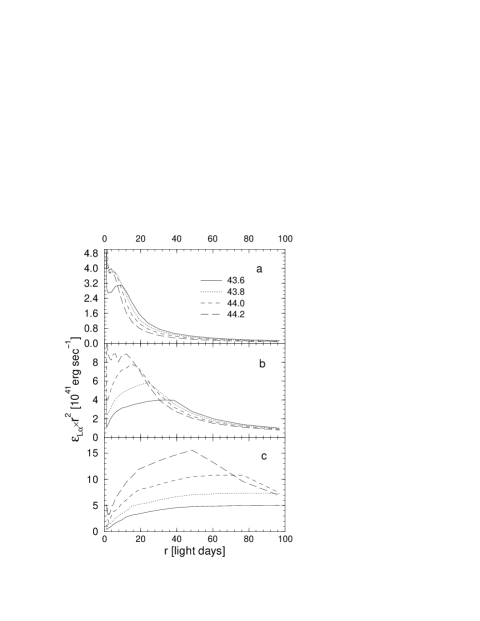
Figure 4.— Ly$\alpha$ emission per unit solid angle versus $r$ for the three densities shown in Fig. 3. a: $N(r=1)=10^{11.7}$ cm^-3. b: $N(r=1)=10^{12.4}$ cm^-3. c: $N(r=1)=10^{13.2}$ cm^-3. For each model there are four different ionizing luminosities, as marked.

Figure 5.— Simulated light-curves (continuous lines) compared with observations for a model with $s=2$, $p=1.5$, $N(r=1)=10^{12.4}$ cm^-3, $N_{col}(r=1)=10^{24}$ cm^-2, $r_{in}=3$ lds, and $r_{out}=25$ lds. The solid lines represent models with different normalization factors for different lines. Dashed lines represent models where the same normalization factor is used for all lines (i.e. a single optimized covering factor)

Figure 6.— Line emission per unit solid angle versus $r$ for the 5 emission lines modeled in Fig. 5.

Figure 7.— Simulated light-curves compared with observations for models with $s=1$, $N(r=1)=10^{11.4}$ cm^-3, $N_{col}(r=1)=10^{24}$ cm^-2, $r_{in}=3$ lds and $r_{out}=100$ lds: solid line - $p=1$ ; dotted line - $p=1.5$ ; dashed line - $p=2$. Note that $p=2$ model is, by far, the best.

Figure 8.— Different SEDs used in this work (see text for details). We show the SED illuminating a cloud positioned at $r=10$ lds with $N=10^{10.4}$ cm^-3 and $N_{col}=10^{23.3}$ cm^-2.

Figure 9.— Same as Fig. 7 for a model with variable shape SED (Fig. 8d).