An analytic study of Bondi–Hoyle–Lyttleton accretion

Abstract

The adiabatic shock produced by a compact object moving supersonically relative to a gas with uniform entropy and no vorticity is a source of entropy gradients and vorticity. We investigate these analytically. The non–axisymmetric Rayleigh–Taylor and axisymmetric Kelvin–Helmholtz linear instabilities are potential sources of destabilization of the subsonic accretion flow after the shock. A local Lagrangian approach is used in order to evaluate the efficiency of these linear instabilities. However, the conditions required for such a WKB type approximation are fulfilled only marginally: a quantitative estimate of their local growth rate integrated along a flow line shows that their growth time is at best comparable to the time needed for advection onto the accretor, even at high Mach number and for a small accretor size. Despite this apparently low efficiency, several features of these mechanisms qualitatively match those observed in numerical simulations: in a gas with uniform entropy, the instability occurs only for supersonic accretors. It is nonaxisymmetric, and begins close to the accretor in the equatorial region perpendicular to the symmetry axis. The mechanism is more efficient for a small, highly supersonic accretor, and also if the shock is detached.

We also show by a 3–D numerical simulation an example of unstable accretion of a subsonic flow with non–uniform entropy at infinity. This instability is qualitatively similar to the one observed in 3–D simulations of the Bondi–Hoyle–Lyttleton flow, although it involves neither a bow shock nor an accretion line.

1 Introduction

The instability of the supersonic axisymmetric Bondi–Hoyle–Lyttleton (hereafter BHL) accretion was first discovered in 2–D numerical simulations by Matsuda et al. (1987) for axisymmetric accretion and by Fryxell & Taam (1988), Taam & Fryxell (1989) for flows including density or velocity gradients. The shock surface oscillates from one side of the accretor to the other (so called “flip–flop” instability), leading to high–amplitude, quasi–periodic variations of the mass accretion rate. This phenomenon was later confirmed by Matsuda et al. (1989, 1991, 1992), who showed that this process is more violent for small accretor sizes, non absorbing accretors, and high Mach numbers (see also Benensohn et al. 1997, Shima et al. 1998). 3–D numerical simulations were performed by Ishii et al. (1993), Ruffert (1996 and previous works for homogeneous media and 1997 for flows including gradients), showing again quasi–periodic variations of the mass accretion rate, although with a smaller amplitude (up to 30 per cent), and with deformations of the shock surface only in the immediate vicinity of the accretor.

Livio (1992) proposed a series of possible observational implications of the instability. In particular, it ought to occur in the accretion process of a neutron star orbiting in a dense wind in high mass X-ray binaries (HMXB) (Taam et al. 1988, De Kool & Anzer 1993). It was also applied to the supermassive black hole SgrA^∗ at the galactic center (Ruffert and Melia 1994), and even to individual galaxies in the intracluster gas (Balsara et al. 1994).

Accretion onto a point like Newtonian accretor moving supersonically in a uniform adiabatic gas is of course a highly idealized problem. It presents the advantage of depending only on two dimensionless parameters, namely the adiabatic index $\gamma$ of the gas and its mach number ${\cal M}_{\infty}$ at infinity. Although this academic formulation seems simple, it gives rise to an instability for which no clear criterion is available yet. The extreme simplicity of this formulation leads us to expect simple laws describing the onset of instability, and in particular the distribution of timescales characterizing the instability. Numerical simulations have to include a third dimensionless parameter, namely the size of the accretor $r_{*}$ in units of the accretion radius ($r_{\rm A}\equiv 2GM/v_{\infty}^{2}$). Due to prohibitive computationnal cost, the smallest accretor size considered in 3–D was $r_{*}/r_{\rm A}=0.02$ (Ruffert 1996 and previous works). We would like to be able to extrapolate the results obtained with numerical simulations to smaller accretors, like a weakly magnetized neutron star or a black hole, moving at $v_{\infty}=1000$ km s^-1, for which $r_{*}/r_{\rm A}\sim 10^{-5}$.

Despite numerous numerical simulations, our understanding of the instability is still unsatisfactory. The instability of the accretion column for cold flows is well established (Cowie 1977, Soker 1990, 1991), but does not directly apply to the case of hydrodynamic BHL flows. A tentative explanation for the flip–flop instability was proposed by Livio et al. (1991), who showed that a conical shock becomes unstable when its opening angle exceeds a critical value. However, recent numerical simulations (Ruffert 1994b, 1995) suggest that the origin of the instability in 3–D is to be found within the subsonic flow near the accretor rather than at the shock surface. This lack of a definite physical explanation for the instability left open the question of whether this instability is influenced by numerical artifacts or is a natural consequence of the physics involved.

A detailed understanding of the instability mechanism should enable us to predict how the instability is influenced by the effects of the accretor size, density and velocity gradients in the upstream flow (Ruffert & Anzer 1995, Ruffert 1997), radiative cooling and heating of the gas (Blondin et al. 1990, Taam et al. 1991) and relativistic effects near the accretor (Petrich et al. 1989, Font & Ibanez 1998a,b), and be more confident in invoking this instability for the variability of accreting systems in astrophysics.

To suggest such a physical mechanism is the purpose of the present paper.

The local approach that we use is shortly reviewed in Sect. 2. A lower bound for the entropy gradient produced by a shock is computed in Sect. 3. We use a simplified formulation of the Rayleigh–Taylor (Sect. 4) and Kelvin–Helmholtz (Sect. 5) linear instabilities in order to estimate their influence on the stationary BHL flow described in Foglizzo & Ruffert (1997, Paper I). They are compared and discussed in Sect. 6. The results of new subsonic 3-D simulations are interpreted in the light of this analysis in Sect. 7.

2 Local stability analysis

2.1 Local linear growth rate integrated along a flow line

According to the numerical simulations (e.g. Ruffert 1995), the instability of the BHL flow occurs only when a shock is present. The shock is a source of entropy inhomogeneities and vorticity, and therefore potentially a source for two well known local instabilities: entropy gradients in a gravitational field may lead to the Rayleigh–Taylor instability (hereafter RTi ), and vorticity can induce the Kelvin–Helmholtz instability (hereafter KHi ). Note that entropy gradients ${\@vec{\nabla}}S$ and vorticity ${\@vec{w}}$ in the BHL flow are closely related by Eq. (10) in Paper I:

$${\@vec{w}}\times{\@vec{v}}=T{\@vec{\nabla}}S.$$ (1)

Unlike Garlick (1979) and Petterson et al. (1980) who used a global analysis to show the stability of the spherically symmetric accretion flows, we adopt here a local approach to estimate the effect of the RTi and KHi on the axisymmetric BHL flow. Although a global perturbative analysis would in principle lead to conclusive statements about the stability of the flow, it seems to be excessively difficult for axisymmetric flows, where a boundary value problem must be solved in two dimensions (radial and azimuthal) for perturbations of an incompletely known stationary flow (Paper I). The local approach has the double advantage of being mathematically tractable and physically understandable, although it might require some strong approximations. Using the same notation as in Paper I, flow lines are indexed by their distance $\varpi$ to the symmetry axis at infinity. We evaluate the typical local growth rate of each instability and integrate it over the time available for amplification, i.e. along a flow line $\varpi$ between the shock $r_{\rm sh}(\varpi)$ and the accretor surface $r_{\star}(\varpi)$. We would like to check whether such a mechanism can amplify perturbations up to non–linear amplitudes before they are advected onto the surface of the accretor. We consider the linear growth rate $|\sigma_{i}({\@vec{r}})|$ of the instability ($i=$ RT or KH) as obtained from a normal mode approach in an infinite medium of same entropy gradient and vorticity as at the position ${\@vec{r}}$ in the BHL flow. As stressed by Garlick (1979) in the case of spherical accretion, such a local approximation is justified only if the distance over which the growth rate varies $(\partial\log\sigma_{i}/\partial r)^{-1}$ is longer than the distance $(v/\sigma_{i})$ traveled during a growth time. The variation of the growth rate is due to the convergence and acceleration of the flow, typically on a scale $r$. The criterion can be stated quantitatively as follows:

$$\left|{\sigma_{i}({\@vec{r}})r\over{\@vec{v}}}\right|\gg\left|{\partial\log\sigma_{i}\over\partial\log r}\right|\sim 1\;.$$ (2)

We estimate the quantity ${\cal A}_{i}(\varpi)$ defined as:

$${\cal A}_{i}(\varpi) \equiv \int_{t_{\rm sh}}^{t_{\star}}|\sigma_{i}({\@vec{r}})|{\rm d}t=\int_{{\@vec{r}}_{\rm sh}(\varpi)}^{{\@vec{r}}_{\star}(\varpi)}{|\sigma_{i}({\@vec{r}})|\over v({\@vec{r}})}{\rm d}l\;,$$ (3)

$${\hat{\cal A}_{i}} \equiv {\rm Max}\{{\cal A}_{i}(\varpi),\varpi>0\},$$ (4)

where we defined the elementary displacement as ${\rm d}l\equiv v{\rm d}t$. ${\hat{\cal A}_{i}}$ is a dimensionless number which depends on the three dimensionless parameters of the problem, namely the Mach number ${\cal M}_{\infty}\geq 0$ of the flow at infinity, the adiabatic index $5/3\geq\gamma\geq 1$ and the accretor radius $r_{\star}\geq 0$. We aim at determining the maximum value of ${\hat{\cal A}_{i}}$ when these parameters are varied.

The WKB approximation gives accurate results where its criterion (2) is satisfied, i.e. if ${\hat{\cal A}_{i}}\gg 1$. A threshold ${\hat{\cal A}_{i}}^{*}$ exists above which the results are still significant, e.g. within $10\%$. As shown by Bender & Orszag (1978) in many illustrative examples of the WKB method, the WKB approximation often gives reliable results even when its criterion is marginally satisfied. Although this may lead us to expect ${\hat{\cal A}_{i}}^{*}\sim 1$, the threshold ${\hat{\cal A}_{i}}^{*}$ does not always strictly equal unity and naturally depends on the problem considered. The exact determination of ${\hat{\cal A}_{i}}^{*}$ lies beyond the scope of this paper, and we shall assume it is of the order of unity. The three following situations might be encountered:

(i) if ${\hat{\cal A}_{i}}\gg{\hat{\cal A}_{i}}^{*}$, we conclude that the criterion (2) is fulfilled, and that a strong linear instability is identified for the corresponding set of parameters.

(ii) If ${\hat{\cal A}_{i}}>{\hat{\cal A}_{i}}^{*}$ is finite, we would conclude that a marginal linear instability is present, which may lead to a non–linear instability or saturation if the typical amplitude of the perturbations is larger than $\exp(-{\hat{\cal A}_{i}})$. For example, ${\hat{\cal A}_{i}}\sim 3$ would be enough to amplify to non–linear amplitudes initial perturbations of order $5\%$.

(iii) If ${\hat{\cal A}_{i}}<{\hat{\cal A}_{i}}^{*}$, the criterion (2) is not fulfilled and our method does not allow us to reach a conclusive statement.

Note that none of the 3–D numerical simulations suggest a particularly violent linear instability, since several accretion times $r_{\rm A}/c_{\infty}$ are usually needed before the instability becomes visible (e.g. Ruffert 1995). Case (i) is therefore a priori excluded in the range of parameters covered by these simulations, i.e. ${\cal M}_{\infty}\leq 10$, $r_{\star}/r_{\rm A}\leq 0.02$.

2.2 Local expansion in the vicinity of a point like accretor

Our local approach makes the important “continuity” assumption that the BHL flow on a Newtonian accretor of size $r_{\star}$ resembles the BHL flow on a point like Newtonian accretor when $r_{\star}\to 0$. This allows us to make series expansions in the vicinity of the singularity $r=0$, and check whether ${\hat{\cal A}_{i}}$ diverges when $r_{\star}\to 0$. Although the limit $r\to 0$ with Newtonian gravity is unrealistic (see e.g. Petrich et al. 1989, Font & Ibanez 1998a,b for relativistic effects), it is useful in order to understand formally classical flows, before more sophisticated effects are added.

3 Entropy distribution produced by the shock

3.1 Entropy gradient along the shock

For the sake of simplicity, in what follows we choose the same units as in Paper I, such that the ratio of the mean molecular weight to the gas constant $\mu/{\cal R}=1$, without loosing any generality. The Rankine-Hugoniot conditions (e.g. Landau & Lifshitz 1987) imply that the entropy jump $\Delta S$ across an adiabatic shock is an increasing function of the Mach number ${\cal M}_{1}$ associated to the velocity component $v_{1\perp}$ ahead of and perpendicular to the shock:

$${\rm e}^{\Delta S}=\left[{2+(\gamma-1){\cal M}_{1}^{2}\over(\gamma+1){\cal M}_{1}^{2}}\right]^{\gamma\over\gamma-1}\left[{2\gamma{\cal M}_{1}^{2}-\gamma+1\over\gamma+1}\right]^{1\over\gamma-1}\;.$$ (5)

Let $v_{2\perp}$ be the velocity component perpendicular to and immediately after the shock. We write the entropy gradient immediately after the shock as a function of ${\cal M}_{1}$ and its variations with respect to the curvilinear abscisse $L$ along the shock, using Eq. (5):

$$\nabla S = {2\eta\over\gamma-1}{v_{2}\over v_{2\perp}}{\partial\log{\cal M}_{1}\over\partial L},$$ (6)

$$\eta \equiv {2\gamma(\gamma-1)({\cal M}_{1}^{2}-1)^{2}\over(2+(\gamma-1){\cal M}_{1}^{2})(2\gamma{\cal M}_{1}^{2}-(\gamma-1))}<1.$$ (7)

$\eta$ always converges to unity for large Mach numbers, when the kinetic energy of the gas exceeds its internal energy (i.e. ${\cal M}_{1}^{2}\gg 2/(\gamma-1)$). The convergence is thus much slower for $\gamma$ close to 1 (Fig. 1).

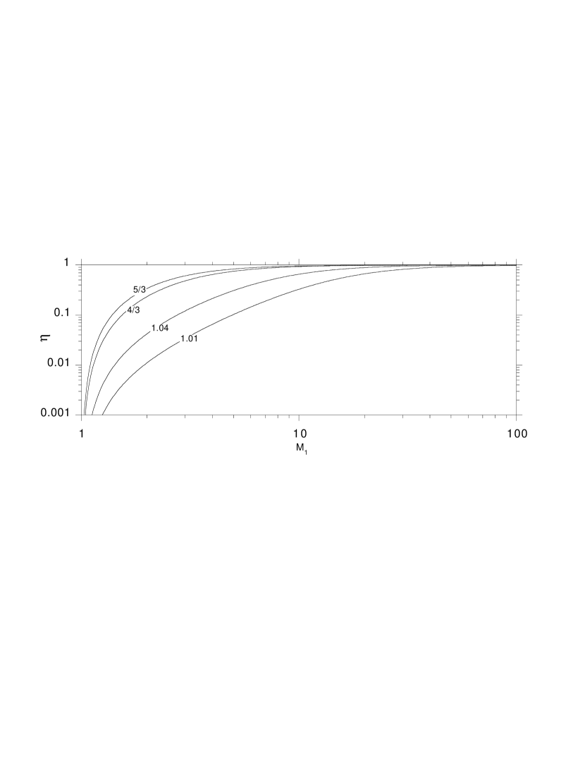
Figure 1: Coefficient $\eta<1$ entering the expression (6) of the entropy gradient created by the shock. The value of the adiabatic index $\gamma$ is indicated on each curve.

According to numerical simulations, the shock distance seems to vary strongly from about 0.2 accretion radii for $\gamma=5/3$ to apparently zero for $\gamma=1.01$ ($r_{\star}=0.02$ in Ruffert 1996). It is not clear yet whether the shock would be detached for smaller accretors. Wolfson (1977) remarked that for $\gamma$ close to one, energy is soaked up by the internal degrees of freedom of the gas, therefore not contributing to support the shock through the kinetic pressure, thus favouring an attached shock. This leads us to consider successively the cases of attached and detached shock.

3.2 Case of a shock attached to a point like accretor

We deduce from Eqs. (E1), (E2), (E4) in Paper I that along a shock attached to a point like accretor with an angle $\theta_{\rm sh}$, for $r\ll r_{\rm A}$, the velocity scales like:

$$v_{1\perp} = \left({2GM\over L}\right)^{1\over 2}\cos{\theta_{\rm sh}\over 2}\sim{\gamma+1\over\gamma-1}v_{2\perp},$$ (8)

$$v_{1\parallel} = \left({2GM\over L}\right)^{1\over 2}\sin{\theta_{\rm sh}\over 2}=v_{2\parallel}.$$ (9)

Using Eq. (6), the entropy gradient immediately after the shock, close to the point like accretor is:

$$\left|\nabla S\right|\sim{1\over\gamma-1}\left[1+\left({\gamma+1\over\gamma-1}\right)^{2}\tan^{2}{\theta_{\rm sh}\over 2}\right]^{1\over 2}{1\over L}.$$ (10)

The entropy produced by the shock is a decreasing function of $L$ if the shock is attached. It depends on the Mach number only through the shock opening angle $\theta_{\rm sh}$.

3.3 Case of a detached axisymmetric shock

Let ${r}_{\rm sh}(\theta)$ be the shape of the axisymmetric shock surface, using polar coordinates $(r,\theta)$ centred on the accretor.

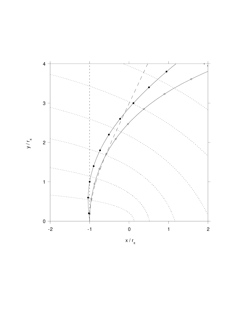
Figure 2: The coordinates of the accretor are $(0,0)$ on the upper plot. The hyperbolic trajectories of the gas emanating from $x<0$ are represented by dotted lines. Four particular shock shapes are plotted for $r_{\pi}=0.1$ accretion radii. The short dash line is orthogonal to the symmmetry axis, and the long dash curve is orthogonal to the supersonic flow lines. The curves with circles are the optimal shapes leading to the smallest entropy gradients corresponding to polynomial shapes of the variable $y^{2}$ (empty circles) and $y^{1/2}$ (filled circles). The value of $\zeta$ along these four curves is displayed on the bottom plot.

Let $r_{\pi}\equiv{r}_{\rm sh}(\pi)$ be the distance of the shock from the accretor, along the symmetry axis. Eq. (5) indicates that when ${\cal M}_{\infty}\gg 1$, the entropy jump along the symmetry axis is:

$$\Delta S(r_{\pi})\sim{2\over\gamma-1}\log{\cal M}_{1}\geq{2\over\gamma-1}\log{\cal M}_{\infty}\;.$$ (11)

Far from the accretor, the shock surface approaches the Mach cone of semi-angle $\theta_{s}$ defined by $\sin\theta_{s}\equiv 1/{\cal M}_{\infty}$ (${\cal M}_{1}\sim 1$). The entropy jump therefore decreases from $\Delta S(r_{\pi})$ ahead of the accretor to zero far from it. Since the entropy gradient immediately after the shock surface vanishes both on the symmetry axis and far from the accretor, the maximum entropy gradient $\left|\nabla S\right|_{\rm max}$ is reached on a circle ${r}_{\rm sh}(\theta_{\rm max})$ corresponding to an intermediate azimuthal angle $\theta_{\rm max}$.
Let us denote by $\alpha$ the angle between the flow line and the vector perpendicular to the shock surface, before the shock, so that $v_{1\perp}=v_{1}\cos\alpha$. Defining the dimensionless function $\zeta$ along the shock surface ${r}_{\rm sh}(\theta)$ as

$$\zeta({r}_{\rm sh}(\theta))\equiv-{r_{\pi}\over\cos\alpha}{\partial\log{\cal M}_{1}\over\partial L}\leq\zeta_{\rm max},$$ (12)

Eq. (6) is rewritten as follows:

$$\nabla S = -{2\eta\over\gamma-1}\left[1+\left({v_{1\perp}^{2}\over v_{2\perp}^{2}}-1\right)\sin^{2}\alpha\right]^{1\over 2}{\zeta\over r_{\pi}},$$ (13)

$$1 < {v_{1\perp}\over v_{2\perp}}={(\gamma+1){\cal M}_{1}^{2}\over 2+(\gamma-1){\cal M}_{1}^{2}}<{\gamma+1\over\gamma-1}.$$ (14)

The Rankine-Hugoniot condition (Eq. 14) and Eq. (13) provide us with both a lower and an upper bound for the maximum entropy gradient produced by a strong shock ($\eta\sim 1$ for ${\cal M}_{\infty}\gg 1$):

$${2(\gamma+1)\over(\gamma-1)^{2}}{\zeta_{\rm max}\over r_{\pi}}\geq\left|\nabla S\right|_{\rm max}\geq{2\over\gamma-1}{\zeta_{\rm max}\over r_{\pi}}.$$ (15)

The value of the maximum $\zeta_{\rm max}$ of the function $\zeta$ depends only on the properties of the supersonic flow before the shock, and on the shape of the shock surface ${r}_{\rm sh}(\theta)$. The function $\zeta^{*}(r_{\pi})$ is defined as the minimum value of $\zeta_{\rm max}$ for all possible continuous mathematical curves ${r}_{\rm sh}(\theta)$ satisfying ${r}_{\rm sh}(\pi)=r_{\pi}$ and ${\rm d}{r}_{\rm sh}/{\rm d}\theta(\pi)=0$:

$$\zeta^{*}(r_{\pi})\equiv{\rm Min}\;\left\{\zeta_{\rm max},\;{\rm any\;curve}\;r_{\rm sh}(\theta)\;,{r}_{\rm sh}(\pi)=r_{\pi}\right\}.$$ (16)

Thus we obtain a lower bound for the maximum entropy gradient $|\nabla S|_{\rm max}$ produced by a detached shock standing at the distance $r_{\pi}$ from the accretor:

$$\left|\nabla S\right|_{\rm max}\geq{2\over\gamma-1}{\zeta^{*}\over r_{\pi}}.$$ (17)

Figure 3: Coefficient $\zeta^{*}$ characterizing the minimum value of the maximum entropy gradient immediately after an axisymmetric shock, depending on its distance $r_{\pi}$ to the accretor. The shock shapes are the same as in Fig. 2.

In the framework of the approximation of the supersonic trajectories by hyperbolae, for ${\cal M}_{\infty}\gg 1$, $\zeta^{*}$ depends only on the distance $r_{\pi}$ of the shock. We have computed numerically the function $\zeta^{*}(r_{\pi})$ using a polynomial approximation of the shock shape and a downhill simplex method for the minimization (Press et al. 1992). Powell’s method was also used with comparable results. Satisfactory results were obtained with a polynomial $x(y)$ of order 3 in $y^{2}$. The overall minimum seems to be reached by the singular curve scaling like $x+r_{\pi}\sim y^{3/2}$ near the symmetry axis, which can be approached by a series of regular polynomials (Figs 2 and 3). For comparison, a plane shock orthogonal to the symmetry axis produces typically twice as much entropy gradients than the minimum value ($\zeta_{\rm max}/\zeta^{*}\sim 2$). More realistic is the curve orthogonal to the supersonic flow lines ($\alpha\equiv 0$), which produces entropy gradients about $20\%$ stronger than the absolute minimal value. According to Fig. 3, the coefficient $\zeta^{*}>0.1$ for realistic shock distances, i.e. $r_{\pi}<r_{\rm A}$. The maximum entropy gradient along the shock stands near $L\sim r_{\pi}$ (Fig. 2).

Fig. 2 shows that the mathematical curves approaching the minimum value of the entropy gradient after the shock are not very different from the physical shock shapes observed in numerical simulations (e.g. Fig. 7). The lower bound $\zeta^{*}$ might therefore be a good approximation of the realistic value of $\zeta_{\rm max}$, within a factor two.

3.4 Entropy gradient in the subsonic flow between a detached shock and the accretor

If the boundary condition on the surface of the accretor allows a high enough mass accretion rate, the maximum entropy gradient immediately after the shock corresponds to a flow line $\varpi_{\rm max}$ converging to the accretor. With the entropy remaining constant along each flow line after the shock, the gradient of entropy across the flow is simply the gradient immediately after the shock surface modified by a geometrical factor. If the convergence towards the accretor were along straight flow lines, the entropy gradient would simply increase like $1/r$. However, flow lines are not radial, and we can take this into account by including a geometrical factor $\delta({\@vec{r}})$, so that the distance between two neighbouring flow lines converging towards the accretor scales like $r/\delta({\@vec{r}})$:

$$\delta({\@vec{r}})\equiv{r(\theta)\over{r}_{\rm sh}}{\nabla S({\@vec{r}})\over(\nabla S)_{\rm sh}}\;,$$ (18)

where $r(\theta)$ is the shape of the flow line $\varpi_{\rm max}$, and $(\nabla S)_{\rm sh}$ is the entropy gradient on this flow line immediately after the shock, at a distance ${r}_{\rm sh}$, so that $\delta({\@vec{r}}_{\rm sh})=1$. We made a distinction in Sect. 4 of Paper I between the directions of regular and singular accretion on a point like accretor. The distance between adjacent accreted flow lines decreases like $\sim r$ when $r\to 0$ in a direction of regular accretion ($\lim_{r\to 0}\delta(r)$ is finite), whereas it decreases much faster in a direction of singular accretion ($\lim_{r\to 0}\delta(r)$ diverges). Since we proved in Paper I that accretion for a gas with $\gamma=5/3$ is always regular, we know that the instability of the BHL flow does not rely on the presence of directions of singular accretion. We can therefore assume that $\lim_{r\to 0}\delta$ is finite in our analysis of the instability.

We obtain from Eqs. (15) and (18) upper and lower bounds for the entropy gradient between the detached shock and the accretor, along the flow line $\varpi_{\rm max}$, at high Mach number:

$${2(\gamma+1)\zeta_{\rm max}\over(\gamma-1)^{2}}{{r}_{\rm sh}\over r_{\pi}}{\delta\over r}\geq\left|\nabla S\right|_{\rm max}\geq{2\zeta_{\rm max}\over\gamma-1}{{r}_{\rm sh}\over r_{\pi}}{\delta\over r}\;.$$ (19)

Note that the ratio ${r}_{\rm sh}/r_{\pi}$ is of the order of $2^{1\over 2}$ in Fig. 2.

4 Rayleigh–Taylor instability

4.1 A simplified formulation of the RT instability

Let us consider a stratified gas in a gravitation field. An entropy gradient can act either in a stabilizing or destabilizing manner depending on whether it does or does not contribute to support the gas against gravity. The vertical gravity field ${\@vec{g}}$ and pressure forces at equilibrium are related as follows:

$${\@vec{g}}={1\over\rho_{0}}{\@vec{\nabla}}P_{0}\;.$$ (20)

The Brunt–Väisälä frequency $N$ is the frequency of oscillations of the stratified gas, in the limit of small wavelengths perpendicular to the gravity field (see Appendix A.1). $\sigma_{\rm RT}\equiv(-N^{2})^{1\over 2}$ is the local growth rate of the RTi when the entropy decreases upwards:

$$\sigma_{\rm RT}^{2}\equiv-N^{2}\equiv{\gamma-1\over\gamma}{\@vec{g}}\cdot{\@vec{\nabla}}S\;.$$ (21)

If the flow is sheared with height, perturbations with a short horizontal wavelength in the direction perpendicular to the flow velocity grow at the same rate (see Appendix A.1).

4.2 Effective gravity in the comoving frame

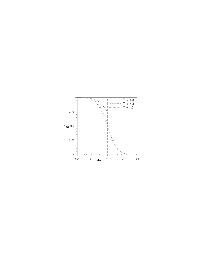
Figure 4: Effective gravity, in $GM/r^{2}$ units, in the case of spherical accretion for various values of $\gamma$.

From the principle of equivalence, there would be no RTi in a gas falling freely in a gravitational potential, because the effective gravity would then be zero. So in a reference frame falling with the gas, the effective gravity $g_{\rm eff}$ driving the RTi is opposite to the pressure force:

$${\@vec{g}}_{\rm eff}\sim{1\over\rho}{\@vec{\nabla}}P\;.$$ (22)

According to Sect. 4.6 in Paper I, the pressure close to the accretor is spherically symmetric to first order for $\gamma=5/3$. This leads us to neglect the negative contribution of the azimuthal pressure force to the scalar product ${\@vec{\nabla}}P\cdot{\@vec{\nabla}}S$ in Eq. (21). The radial pressure support decreases from the subsonic region to the supersonic region. The effective gravity, calculated analytically in the case of spherical accretion, is displayed in Fig. 4 for various adiabatic indices. In the subsonic region, the effective gravity is more than $50\%$ of the gravity of the accretor for any value $1<\gamma<5/3$. The best pressure support is reached, of course, for $\gamma=5/3$, for which the effective gravity in the subsonic region is at least $75\%$ of the gravity. We shall assume that the effective gravity for an axisymmetric flow is comparable to the effective gravity in the spherical case, thus constraining the dimensionless gravity parameter $g^{*}\in[0.5,1]$ in the subsonic region of the flow:

$$g^{*}\equiv g_{\rm eff}{r^{2}\over GM}.$$ (23)

4.3 RTi efficiency in the BHL flow

4.3.1 General expression of the RT efficiency

According to Eq. (21), the local growth rate of nonaxisymmetric perturbations with a short wavelength perpendicular to both the flow lines and the radial direction (similar to the case $k_{x}\to\infty$, $k_{y}=0$ in Appendix A.1) is approximated as follows:

$$\sigma_{\rm RT}^{2}={\gamma-1\over\gamma}g^{*}{GM\over r^{2}}|\nabla S|\sin\beta\;,$$ (24)

where $\beta$ is the angle between the flow line and the radial direction:

$$\tan\beta\equiv{v_{\theta}\over v_{r}}.$$ (25)

The perpendicular wavelength of a non axisymmetric perturbation decreases geometrically as the flow is advected, so that the growth rate of the RTi stays maximum.

Defining the free fall velocity $v_{\rm ff}$ as

$$v_{\rm ff}\equiv\left({2GM\over r}\right)^{1\over 2},$$ (26)

the integrated efficiency of the RTi defined by Eq. (3) follows from Eqs. (24) and (26) :

$${\cal A}_{\rm RT}(\varpi) \equiv \left({\gamma-1\over 2\gamma}\right)^{1\over 2}\times$$ (27)

$$\int_{{\@vec{r}}_{\rm sh}(\varpi)}^{{\@vec{r}}_{\beta}(\varpi)}g^{*{1\over 2}}{v_{\rm ff}\over v}\left(r|\nabla S|\right)^{1\over 2}\sin^{1\over 2}\beta{{\rm d}l\over r}\;.$$

With the estimates of the entropy gradient and effective gravity of Sects. 3 and 4.2, we are now able to evaluate Eq. (27) for the different topologies discussed in Paper I. Since the entropy along the shock decreases away from the symmetry axis, the stratification is potentially linearly unstable only in the region where $\beta>0$. The conservation of angular momentum implies that $\beta>0$ in the supersonic flow before the shock. Since $\beta$ is likely to increase across the shock, we conclude that the stratification is locally unstable immediately after the shock surface. We denote by $r_{\rm\beta}(\theta)\geq 0$ the surface where the velocity is radial, thus delimiting a region of unstable stratification.

4.3.2 Attached shock

Using Eqs. (10), (24) close to accretor ($\eta\sim 1$), and the relation $\sin\beta=v_{2\perp}/v_{2}$, the local growth rate is:

$$\sigma_{\rm RT}=\left({g^{*}\over 2\gamma}\right)^{1\over 2}{v_{\rm ff}\over r}.$$ (28)

This growth rate must be integrated along a flow line $\varpi$ between the azimuthal angles $\theta_{\rm sh}$ and $\theta_{\rm so}$ corresponding to the shock and the sonic surfaces respectively. The length of this path of integration is of the order of $r(\theta_{\rm sh}-\theta_{\rm so}$). Estimating the velocity after the shock from Eqs. (8) and (9) gives:

$${\cal A}_{\rm RT}(\varpi) \equiv \int^{\theta_{\rm so}}_{\theta_{\rm sh}}{\sigma_{\rm RT}\over v}{\rm d}l,$$ (29)

$$\sim {\gamma+1\over 2\gamma}\left({g^{*}\over 2}\right)^{1\over 2}{\theta_{\rm sh}-\theta_{\rm so}\over\left[\sin^{2}{\theta_{\rm sh}\over 2}+{(\gamma-1)^{2}\over 4\gamma}\right]^{1\over 2}}<2^{1\over 2}.$$ (30)

The efficiency depends strongly on the azimuthal size of the subsonic region reaching the accretor ($\theta_{\rm sh}-\theta_{\rm so}$). This parameter is unfortunately unknown, and we only obtain an upper bound on the efficiency of the RTi : the timescale of the RTi instability is at best comparable to the advection timescale for a shock attached to the accretor, however small the accretor might be.

4.3.3 Region of supersonic accretion near a point like accretor with a detached shock, $\gamma<5/3$

The sign of $\beta$ in the supersonic region might simply preclude the instability ($\beta<0$ for $\gamma=5/3$). Let us show that even if the flow lines were bent in the unstable direction ($\beta>0$ for $\gamma\sim 1$), the RTi would become negligible when the gas approaches a point like accretor. For this we wish to check that the divergence of the entropy gradient when $r\to 0$ is not fast enough to make the RTi growth time shorter than the free fall time. Using Eq. (19) and Eq. (24), the radial dependence of the RTi growth rate in the supersonic region scales like:

$$\sigma_{\rm RT}(r) = {\cal O}\left(g^{*{1\over 2}}{\beta^{1\over 2}\over r^{3\over 2}}\right)$$ (31)

$$\ll {\cal O}\left(r^{-{3\gamma+1\over 4}}\right),$$ (32)

where we have used Eq. (56) of Paper I for an upper bound of $\beta(r\to 0)$ ($\partial\log\beta/\partial\log r\geq(5-3\gamma)/2$), and the decrease of the effective gravity. Using the free fall approximation of the velocity, the contribution of the region surrounding a point like accretor to the efficiency of the RTi scales like:

$$\int^{{\@vec{r}}}_{0}{\sigma_{\rm RT}\over v}{{\rm d}r\over\cos\beta}\ll{\cal O}\left(r^{5-3\gamma\over 2}\right)\;.$$ (33)

From the convergence of the integral when $r\to 0$ we deduce that the local growth time is much longer than the free fall time, and the RTi can be neglected there if $\gamma<5/3$.

4.3.4 Region of subsonic accretion along the maximum entropy gradient

Since the RTi is driven by the entropy gradient, it is natural to evaluate a lower bound for its efficiency along the flow line $\varpi_{\rm max}$ associated with the maximum entropy gradient, at high Mach number ($\eta\sim 1$), using Eqs. (19) and (27):

$${\hat{\cal A}}_{\rm RT} \geq {\rm Min}\;{\cal A}_{\rm RT},$$ (34)

$${\rm Min}\;{\cal A}_{\rm RT} \equiv \left({\zeta_{\rm max}\over\gamma}{{r}_{\rm sh}\over r_{\pi}}\right)^{1\over 2}\int_{{\@vec{r}}_{\rm sh}}^{{\@vec{r}}_{\beta}}{v_{\rm ff}\over v}(\delta g^{*}\sin\beta)^{1\over 2}{{\rm d}l\over r}\;.$$ (35)

The Bernoulli equation can be written in terms of the free fall velocity, and approximated for ${\cal M}_{\infty}^{2}\gg 2/(\gamma-1)$, inside the sonic radius:

$$v^{2}\left[1+{2\over(\gamma-1){\cal M}^{2}}\right] = v_{\rm ff}^{2}+v_{\infty}^{2}\left[1+{2\over(\gamma-1){\cal M}_{\infty}^{2}}\right],$$ (36)

$$\sim v_{\rm ff}^{2},$$ (37)

where we have neglected $v_{\infty}$ compared to $v_{\rm ff}$ between the shock and the accretor, since the shock distance is typically shorter than the accretion radius ($v_{\rm ff}(r_{\rm A})=v_{\infty}$). The ratio $v_{\rm ff}/v$ decreases in the subsonic region between the shock (${r}_{\rm sh}$) and the sonic point ($r_{\rm sonic}$). Applying Eq. (37) at the sonic point (${\cal M}=1$) and at the shock (${\cal M}\sim{\cal M}_{\rm sh}$), we obtain the following range:

$$\left({\gamma+1\over\gamma-1}\right)^{1\over 2}\leq{v_{\rm ff}\over v}\leq{\gamma+1\over\gamma-1}.$$ (38)

If $\gamma<5/3$, the flow line $\varpi_{\rm max}$ reaches the accretor in the supersonic region, and we know from the preceding section that the contribution of this region to the integral is negligible.

Let us examine each of the terms of Eq. (35) for $\gamma=5/3$, which is supposed to be the most unstable case according to numerical simulations.

(i) $0.75\leq g^{*}\leq 1$ according to Fig. 4, and thus we estimate $g^{*}\sim 0.9$,

(ii) the geometrical factor $\delta$ is finite since accretion with $\gamma=5/3$ is always regular (Paper I), and is assumed to be of the order of unity,

(iii) $2\leq v_{\rm ff}/v\leq 4$ according to Eq. (38), and thus we estimate $v_{\rm ff}/v\sim 3$.

Because these three contributions to the integral are finite, we replace each of them by their mean value and approximate Eq. (35) as follows:

$${\rm Min}\;{\cal A}_{\rm RT}\sim 1.0\;\left({\zeta_{\rm max}\over 0.15}\delta{{r}_{\rm sh}\over 2^{1\over 2}r_{\pi}}\right)^{1\over 2}\int_{{\@vec{r}}_{\rm sh}}^{{\@vec{r}}_{\beta}}\sin^{1\over 2}\beta{{\rm d}l\over r}\;.$$ (39)

We showed in Paper I that $\beta<0$ along the sonic surface for $\gamma=5/3$, thus $r_{\beta}(\varpi)>0$ can be estimated as a fraction of the shock distance $r_{\pi}$. This precludes the possibility that the integral in Eq. (39) might diverge when the size of the accretor is decreased. This further suggest that the efficiency of the RTi instability should not increase much when the accretor size is much smaller than the shock distance ($r_{\star}\ll r_{\pi}$). In order to estimate this efficiency, let us remark from Fig. 7 that $\sin\beta$ is close to unity immediately after the shock (see also numerical simulations as in Fig.2). Since we expect that $\beta>0$ over a sizable fraction of the shock distance, this integral is likely to be of order unity. According to the typical values of $\zeta_{\rm max}$ deduced from Fig. 3, we conclude from Eq. (39) that Min ${\cal A}_{\rm RT}$ is of the order of unity, hardly more. Since the lower and upper bounds in Eq. (19) differ by a factor $(\gamma+1)/(\gamma-1)$, and since the RTi growth rate scales like the square root of the entropy gradient, we finally estimate for $\gamma=5/3$:

$$1.0\la{\hat{\cal A}}_{\rm RT}\la 2.0\;.$$ (40)

Thus the integrated efficiency of the linear RTi does not diverge, even in the case of a point like accretor moving at high Mach number in a gas with $\gamma=5/3$. Although small, this efficiency of order unity is not negligible.

5 Kelvin–Helmholtz instability

5.1 A simplified formulation of the KH instability

The maximum linear growth rate of the KHi in an inviscid fluid is comparable to the maximal vorticity of the flow in equilibrium. From the studies of the instability with various velocity profiles (see an overview in Drazin and Reid, 1981), one can extrapolate the following growth rate $\sigma_{\rm KH}$ and optimal wavelength $\lambda_{\rm max}$ of the instability corresponding to a vorticity profile with a maximum $|w_{\rm max}|$ and a gradient width $h$:

$$|\sigma_{\rm KH}| = \alpha\;|w_{\rm max}|\;\chi({\lambda_{\rm max}\over\lambda}),\quad{\rm with}\,\,\alpha\approx 0.2,$$ (41)

$$\lambda_{\rm max} = \kappa\;h\;,\quad\quad\quad\quad\quad\quad\quad\,{\rm with}\,\,\kappa\approx 7,$$ (42)

where $\chi(x)\leq\chi(1)=1$ is a function of the wavelength $\lambda$ of the perturbation. Its typical shape, obtained by a numerical solution of the Orr-Sommerfeld equation, is plotted in Fig. 5.

Figure 5: Typical dependence of the Kelvin-Helmholtz instability on the wavelength $\lambda$ of the perturbation, described by the function $\chi$ (full line). The dotted line shows the slope at long wavelengths.

The effect of compressibility on the linear instability can be studied by solving the linearized equations for a sheared plane flow (see Appendix A.2), with the following velocity profile:

$$v(z) \equiv {v_{0}\over 2}\tanh{2z\over h},$$ (43)

$$w_{\rm max} = {v_{0}\over h}.$$ (44)

Neither the value of $\gamma$, within the range $[1,5/3]$, nor the presence of an entropy gradient across the flow influences the growth rate and the wavelength of the most unstable mode by more than a few percent.

Figure 6: Maximum growth rate of the linear KHi and associated wavelength, as a function of the Mach number ${\cal M}_{\rm KH}=v_{0}/c_{0}$ for a uniform sound velocity $c_{0}$, and a velocity profile given by Eq. (43). The growth rate $\sigma_{\rm KH}$ is displayed in units of the vorticity maximum $w_{\rm max}=v_{0}/h$ (solid line). The dimensionless parameter $\kappa$ measures the optimal wavelength $\lambda_{\rm max}$ in units of the width of the vorticity peak $h$ (dashed line). The rigid boundaries are at $\pm 5h$. Within the accuracy of our numerical relaxation method, these curves are independent of the adiabatic index in the range of interest $1\leq\gamma\leq 5/3$.

A determining quantity for the KHi in compressible flows is the relative Mach number ${\cal M}_{\rm KH}$ measured in the frame comoving with the flow line of maximum vorticity:

$${\cal M}_{\rm KH}\equiv{|v(h/2)-v(-h/2)|\over c_{0}}\sim{hw_{\rm max}\over c_{0}}\;,$$ (45)

with $c_{0}$ being the sound speed on the line of maximum vorticity ($z=0$), and $v(z)$ the $z$-dependent velocity of the flow in the $y$–direction. The growth rate decreases by a factor of $2$ between the very subsonic flow (which mimics the incompressible case) and ${\cal M}_{\rm KH}=1.3$, as shown on Fig. 6. So the difference of velocities within the vorticity peak must be less than the sound speed (i.e. ${\cal M}_{\rm KH}<1$) in order to allow pressure forces to act in the KHi mechanism as efficiently as in the incompressible limit. Note that the limiting values of $\sigma_{\rm KH}$ and $\kappa$ for ${\cal M}_{\rm KH}\to 0$ in Fig. 6 agree with the values of $\alpha$ and $\kappa$ stated in Eqs. (41) and (42).

5.2 Application to the BHL flow with a detached shock

According to Eq. (1), the same symmetry arguments used for the entropy gradients in Sect. 3 apply to the vorticity. A surface of steepest increase of the vorticity therefore connects the shock to the accretor, where the vorticity diverges for $r\to 0$ (Eqs. 49–59 in Paper I).

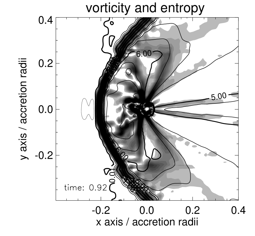
Figure 7: Lines of constant entropy superimposed on a greyscale map of the vorticity in a numerical simulation of BHL with $\gamma=5/3$ and ${\cal M}_{\infty}=10$ (model FS in Ruffert 1994b). In a good approximation, the line of steepest increase of the entropy gradient coincide with the line of steepest increase of the vorticity, and corresponds to a line of flow.

If this surface of maximum vorticity is not too different from a flow surface, the KHi will develop most efficiently along these particular flow lines. Numerical simulations, illustrated by Fig. 7, together with Eq. (1), suggest that the surface of steepest increase of the entropy gradient and the surface of steepest increase of the vorticity coincide with the flow line denoted by $\varpi_{\rm max}$, such that $\theta_{0}(\varpi_{\rm max})$ is a direction of maximum entropy gradient and vorticity.

We use Eqs. (1) and (19) along these flow lines to write the vorticity as follows:

$$w_{\rm max} = {c^{2}\over\gamma v}\nabla S\;,$$ (46)

$$\geq {2\zeta_{\rm max}\over\gamma(\gamma-1)}{\delta\over{\cal M}^{2}}{{r}_{\rm sh}\over r_{\pi}}{v\over r}\;.$$ (47)

$\delta$ is related to the width $h(r)$ of the vorticity peak ($h_{\rm sh}\equiv h({r}_{\rm sh})$), and thus to the optimal wavelength of the KHi , through Eqs. (18) and (42):

$$\delta({\@vec{r}})={h_{\rm sh}\over h(r)}\left({r\over{r}_{\rm sh}}\right)\;.$$ (48)

Although the vorticity defined in Eq. (47) may become arbitrarily large when $\gamma$ is close to unity, the time-scale of the KHi is limited by compressibility effects. Let us estimate the Mach number ${\cal M}_{\rm KH}$ defined in Eq. (45), using Eqs. (47) and (48):

$${\cal M}_{\rm KH}\sim{2\zeta_{\rm max}\over\gamma(\gamma-1)}{h_{\rm sh}\over r_{\pi}}{1\over{\cal M}},$$ (49)

Paradoxically, Eq. (49) indicates that compressibility effects are stronger in subsonic regions. We introduce in Eq. (49) the minimum value ${\cal M}_{\rm sh}$ of the Mach number after the shock, defined by the Rankine–Hugoniot jump conditions:

$${\cal M}_{\rm sh} \equiv \left({\gamma-1\over 2\gamma}\right)^{1\over 2},$$ (50)

$${\cal M}_{\rm KH} \sim {0.4\over\gamma^{1\over 2}(\gamma-1)^{3\over 2}}{\zeta_{\rm max}\over 0.15}\;{h_{\rm sh}\over r_{\pi}}\;{{\cal M}_{\rm sh}\over{\cal M}},$$ (51)

$$\sim 0.6\;{\zeta_{\rm max}\over 0.15}\;{h_{\rm sh}\over r_{\pi}}\;{{\cal M}_{\rm sh}\over{\cal M}},$$ (52)

where Eq. (52) assumes $\gamma=5/3$. Noting that the Mach number increases from the shock to the sonic surface (${\cal M}>{\cal M}_{\rm sh}$), and that $h_{\rm sh}/r_{\pi}$ is of the order of unity, we conclude that the effect of compressibility on the KHi can be neglected for $\gamma=5/3$. From Eq. (41) and (47), we can write the minimum KHi growth rate, at high mach number (${\cal M}_{\infty}\gg 1,\eta\sim 1$), as follows:

$$|\sigma_{\rm KH}|\geq{2\alpha\zeta_{\rm max}\delta\over\gamma(\gamma-1)}\;{\chi\over{\cal M}^{2}}\;{{r}_{\rm sh}\over r_{\pi}}\;{v\over r}\;,$$ (53)

Let us estimate the minimum efficiency Min ${\cal A}_{\rm KH}$ of the KHi mechanism along the flow line $\varpi_{\rm max}$:

$${\rm Min}\;{\cal A}_{\rm KH}(\varpi_{\rm max})\equiv{2\alpha\zeta_{\rm max}\over\gamma(\gamma-1)}{{r}_{\rm sh}\over r_{\pi}}\int_{{r}_{\rm sh}(\varpi_{\rm max})}^{r_{\star}(\varpi_{\rm max})}{\delta\chi\over{\cal M}^{2}}{{\rm d}l\over r}\;.$$ (54)

The width $h$ of the entropy gradient decreases geometrically with $r$, and the optimal wavelength of the KHi decreases according to Eq. (42). By contrast, the wavelength $\lambda$, parallel to the flow line, of a Lagrangian perturbation must increase when advected, since the flow is accelerated. It is therefore not possible to maintain the KHi with its local maximum growth rate during the advection of the perturbation.

If we denote by $\lambda_{\rm i}\equiv\kappa h_{\rm i}\ll{r}_{\rm sh}$ the initial wavelength of the perturbation, Fig. 5 indicates that it becomes unstable only when advected towards a region where the gradient width is $h(r)<2\lambda/\kappa$. We rewrite Eq. (54) using Eq. (48):

$${\rm Min}\;{\cal A}_{\rm KH}={2\alpha\zeta_{\rm max}\over\gamma(\gamma-1)}{{r}_{\rm sh}\over r_{\pi}}\int_{{r}_{\rm sh}}^{r_{\star}}\left[{\chi(h/h_{\rm i})\over h/h_{\rm i}}\right]{1\over{\cal M}^{2}}{h_{\rm sh}\over h_{\rm i}}{{\rm d}l\over{r}_{\rm sh}}\;.$$ (55)

Neglecting the increase of $\lambda_{i}$ due to the acceleration compared to the linear decrease of $h(r)$, the ratio $\lambda_{\rm max}(r)/\lambda_{i}\equiv h(r)/h_{i}$ decreases linearly to zero when $r\to 0$. The integral in Eq. (55) is approximated for $r_{\star}\to 0$ by extracting some average values $\hat{\delta}$ and $\hat{\cal M}$ from it, and integrating the function $\chi$ described in Fig. 5:

$$\int_{0}^{{r}_{\rm sh}}\left[{\chi(h/h_{i})\over h/h_{i}}\right]{1\over{\cal M}^{2}}{h_{\rm sh}\over h_{i}}{{\rm d}l\over{r}_{\rm sh}} \sim {\hat{\delta}\over\hat{\cal M}^{2}}\int_{0}^{2}{\chi(x)\over x}{\rm d}x,$$ (56)

$$\sim 2.1\;{\hat{\delta}\over\hat{\cal M}^{2}},$$ (57)

$${\rm Min}\;{\cal A}_{\rm KH}\sim{0.4\over(\gamma-1)^{2}}\;{\alpha\over 0.2}\;{\zeta_{\rm max}\over 0.15}\;\hat{\delta}\;{{r}_{\rm sh}\over 2^{1\over 2}r_{\pi}}\left({{\cal M}_{\rm sh}\over\hat{\cal M}}\right)^{2}.$$ (58)

Introducing $\gamma=5/3$ into Eq. (58), and approximating $\hat{\cal M}\sim({\cal M}_{\rm sh}+1)/2$ we obtain:

$${\rm Min}\;{\cal A}_{\rm KH}\sim 0.5\;{\alpha\over 0.2}\;{\zeta_{\rm max}\over 0.15}\;{\hat{\delta}}\;{{r}_{\rm sh}\over 2^{1\over 2}r_{\pi}}.$$ (59)

We deduce from Eqs. (19) and (59) an estimate of the KHi efficiency for $\gamma=5/3$:

$$0.5\la{\hat{\cal A}}_{\rm KH}\la 2.0\;.$$ (60)

In particular, ${\hat{\cal A}}_{\rm KH}$ does not diverge when $r_{\star}\to 0$. According to Eq. (56), the integral in Eq. (55) is regular at $r=0$, thus its value should not depend on the accretor size if $r_{\star}\ll r_{\pi}$. Consequently, the KHi efficiency should be little influenced by the size of the accretor if $r_{\star}\ll r_{\pi}$. The above calculation indicates that a whole range of wavelengths leads to comparable efficiencies if $r_{\star}\ll r_{\pi}$. Although the integrated efficiency remains limited, the variability timescale is directly related to the wavelength of the perturbation.

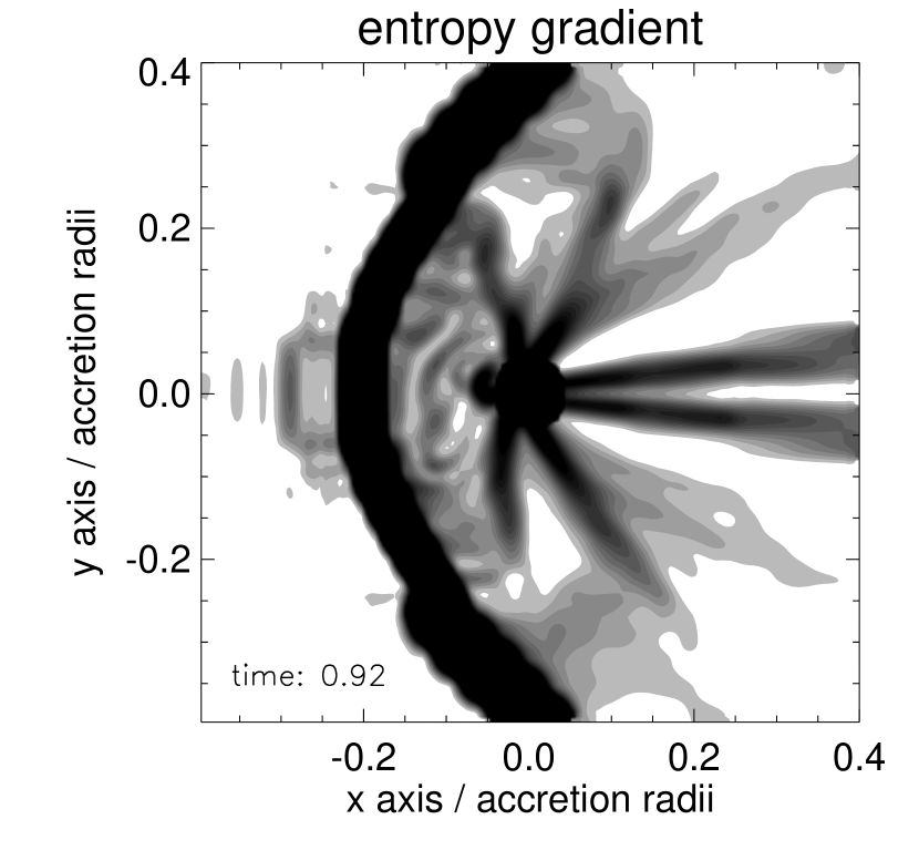
Figure 8: Splitting of the entropy gradient peak generated by the shock into several narrower peaks.

Numerical simulations show that the gradient width, a priori comparable to the radius of curvature of the shock, is split into several maxima of much smaller width, typically of 5–10 degrees in a snapshot of the flow before instability (Fig. 8). One may imagine that the gradient width decreases with time, as more and more gas is accumulated from the downstream side of the accretor, until the gradient width is short enough to start the KHi . We must also note that the generation of vorticity at the interface between the grids in the multi–grid PPM numerical technique might influence the distribution of vorticity in the flow.

6 Discussion of the efficiencies of the two instabilities

The local time scale of the instability in the subsonic region scales like the advection time onto the accretor, so that the efficiency integrated along a flow line is always of order unity (Eqs. 40 and 60). Assuming that the threshold of the WKB approximation is also of the order unity (${\hat{\cal A}_{i}}^{*}\sim 1$) and following the statements of Sect. 2, we stand in the uncomfortable position between case (ii) and case (iii). Despite this uncertainty, it is interesting to compare the analyze the results of numerical simulations in the light of these physical mechanisms.

The efficiency of the instabilities naturally increases with the strength of the shock, as can be seen from the function $\eta({\cal M}_{1})$ (Eq. 7 and Fig. 1). Numerical simulations with $\gamma=4/3$ (Ruffert 1995) and $\gamma=5/3$ (Ruffert & Arnett 1994, Ruffert 1994b) show the same trend: the flow is stable with ${\cal M}_{\infty}=1.4$ and unstable with ${\cal M}_{\infty}=3$ and $10$, with detached shocks in all these situations. The highest entropy gradients are obtained for ${\cal M}_{\infty}^{2}\geq 2/(\gamma-1)$, thus requiring higher Mach numbers for nearly isothermal flows. Increasing the Mach number does not increase the efficiency of the instabilities indefinitely: our estimates show that this efficiency saturates when the increase of the entropy gradient is compensated by the decrease of the advection timescale. We see no obvious justification for a possible divergence of any of the numerous dimensionless parameters introduced ($\zeta,\delta,g^{*},\alpha$) if the Mach number ${\cal M}_{\infty}$ is increased, or if the accretor size is decreased, and therefore expect the integrated efficiencies to be smaller than $2$.

Our calculations seem to indicate that the efficiency should increase when $\gamma$ approaches unity (Eqs. 35, 38 and 58), whereas the most unstable flows observed in simulations correspond to $\gamma=4/3$ and $\gamma=5/3$. Nevertheless, we showed in Sect. 4.3.2 that the efficiency of the RTi is finite for $\gamma=1$ when the shock is attached to the accretor. Thus this paradox would disappear if a critical adiabatic index exists below which the shock is attached to the accretor, as suggested by Wolfson (1977).

The axisymmetric KHi must be considered together with the effect of stratification, which can be stabilizing or destabilizing depending on the sign of $\beta$. The influence of stratification on the KHi can be estimated quantitatively by comparing the time scales associated to each physical process, in the same spirit as was done with the Richardson number. This ratio informs us about a possible stabilization of the KHi by buoyancy forces if $\beta<0$, or which of the two instabilities is the fastest if $\beta>0$. The ratio of the timescales can be deduced from Eqs. (24), (41) and (46) as follows:

$${\sigma_{\rm RT}\over\sigma_{\rm KH}}={1\over\alpha}\left[{\gamma(\gamma-1)\over 2}g^{*}\right]^{1\over 2}{\cal M}^{2}{v_{\rm ff}\over v}{\sin^{1\over 2}\beta\over\chi}\left(r\nabla S_{\rm max}\right)^{-{1\over 2}}.$$ (61)

We estimate this ratio both immediately after the shock and at the sonic point. At the shock, the effective gravity is strong ($g^{*}\sim 1$), and Eqs (19), (38) and (50) provide us with a lower bound for Eq. (61):

$${\sigma_{\rm RT}\over\sigma_{\rm KH}}({r}_{\rm sh}) \geq 3.8(\gamma-1)^{3\over 2}\left({\gamma+1\over\gamma}\right)^{1\over 2}{\sin^{1\over 2}\beta\over\chi}$$ (62)

$$\times \left({0.15\over\delta\zeta_{\rm max}}\right)^{1\over 2}{0.2\over\alpha}\left({2^{1\over 2}r_{\pi}\over{r}_{\rm sh}}\right)^{1\over 2}.$$

Applying this equation to $\gamma=5/3$, we obtain:

$${\sigma_{\rm RT}\over\sigma_{\rm KH}}({r}_{\rm sh})\geq 2.6\;{\sin^{1\over 2}\beta\over\chi}\left({0.15\over\delta\zeta_{\rm max}}\right)^{1\over 2}{0.2\over\alpha}\left({2^{1\over 2}r_{\pi}\over{r}_{\rm sh}}\right)^{1\over 2}.$$ (63)

Since $\beta$ is large immediately after the shock, Eq. (63) suggests that the RTi is more unstable than the KHi there. At the sonic point (${\cal M}=1$), using Eqs. (19) and (38), Eq. (61) becomes:

$${\sigma_{\rm RT}\over\sigma_{\rm KH}}(r_{\rm sonic}) \geq 6.6\gamma^{1\over 2}(\gamma-1){\sin^{1\over 2}\beta\over\chi}$$ (64)

$$\times \left({g^{*}\over 0.75}\right)^{1\over 2}\left({0.15\over\delta\zeta_{\rm max}}\right)^{1\over 2}{0.2\over\alpha}\left({2^{1\over 2}r_{\pi}\over{r}_{\rm sh}}\right)^{1\over 2}.$$

Applying this equation to $\gamma=5/3$, we obtain:

$${\sigma_{\rm RT}\over\sigma_{\rm KH}}(r_{\rm sonic}) \geq 5.7\;{\sin^{1\over 2}\beta\over\chi}$$ (65)

$$\times \left({g^{*}\over 0.75}\right)^{1\over 2}\left({0.15\over\delta\zeta_{\rm max}}\right)^{1\over 2}{0.2\over\alpha}\left({2^{1\over 2}r_{\pi}\over{r}_{\rm sh}}\right)^{1\over 2}.$$

Let us first remark from Eq. (71) of Paper I that if $\gamma=5/3$, $0\leq\lim_{r\to 0}(\partial\log\beta/\partial\log r)\leq 1$, indicating that the convergence of $\sin^{1\over 2}\beta$ towards zero is slower than that of $\chi(r)\sim r/2$ close to a point like accretor. Thus the KHi ultimately becomes stabilized by buoyancy forces near a point like accretor, when the wavelength of the perturbation is much longer than the vorticity gradient width.

According to Eq. (65), a perturbation with a wavelength such that $\chi=1$ at the sonic point would be locally unstable to the KHi with hardly any stabilization by the buoyancy forces if $|\beta|\la 1$ degree. The angle $\beta$ at the sonic point is negative for $\gamma=5/3$ (see Paper I) and much smaller than at the shock, especially if the sonic surface is close to the accretor. We know from Paper I that the sonic surface is attached to the accretor if $\gamma=5/3$. Thus the flow line reaching a point like accretor along the sonic surface is unstable to the KHi without being stabilized by the buoyancy forces. The shortest timescale associated to the KHi therefore depends on the size of the accretor, while the longest is directly related to the shock distance.

Although the RTi is dominant near the shock, and the KHi might prevail closer to the sonic surface, it is hard to disentangle the two mechanisms, which act in a combined way when the shock is detached. The situation is different when the shock is attached to the accretor, since there is no vorticity maximum in this case. It is interesting to note that the linear efficiency estimated in Eq. (30) for an attached shock is not much smaller than the efficiencies derived for a detached shock. Numerical simulations indicate that accretion flows with an attached shock are generally more stable than those with a detached shock (Ruffert 1995, Zarinelli et al. 1995). In the simulations by Ruffert (1996) with $\gamma=1.01$, the instability is nevertheless clearly observed, producing fluctuations of the mass accretion rate of about $7\%$ (simulations with $\gamma=4/3$ and $5/3$ produce typical fluctuations of $14\%$ and $23\%$ respectively). This suggests that the RTi alone may destabilize linearly the flow when the shock is attached, while the combined action of the two mechanisms when the shock is detached is more efficient and leads to higher non linear amplitudes.

7 Instabilities in simulations with subsonic flows

Figure 9: Contour plot of the density distribution together with the instantaneous flow velocities. The contours are spaced logarithmically with intervals of 0.1 dex, the contour corresponding to $10^{0}$ is annotated. The time elapsed since the beginning of the simulation together with the velocity arrow unit is shown at the top right. The accretor is at the center with coordinates $x=0,y=0$. The right figure is a zoom of the left figure enlarged around the accretor.

In order to separate more clearly the different effects that might contribute to the formation of the instabilities, we performed numerical simulations of accretion from a flow with subsonic bulk velocities at infinity, but with a gradient in entropy. The rationale is the following. When the accretor moves supersonically relative to a surrounding medium a bow shock will form. The shock transforms the initially (at infinity) homogeneous medium moving at supersonic velocities into a subsonic flow with an entropy decreasing away from the axis of symmetry.

We did a set of simulations to mimic these conditions, of which we will present here the most important results relevant to the topic of this paper. The accretor radius is chosen to be $r_{\star}=0.02r_{\rm A}$ and the same absorbing boundary conditions are used as in Ruffert (1994a). The simulations are done on 7 nested cartesian grids, the zone size on each finer grid being a factor of two smaller than of the next coarser grid. The largest grid spans 8 accretion radii. Matter is evolved hydrodynamically using the “Piecewise Parabolic Method”, assuming it is a polytropic gas with an adiabatic index of 5/3.

The flow at infinity is in direction of the positive $x$-axis, with a constant velocity along $x$. The pressure is uniform at infinity. In order to maintain pressure equilibrium, the maximum of entropy $\Delta S$ at $y=0$ at infinity along the $x$-axis is offset by a minimum in density with the following shape:

$$\frac{\rho_{\infty}(x,y,z)}{\rho_{\rm 0}} \equiv 1-\varepsilon\exp\left(-\frac{y^{2}}{2}\right)\;,$$ (66)

$${\rm with}\;\varepsilon \equiv 1-\exp\left[-{\gamma-1\over\gamma}\Delta S\right]\;.$$ (67)

The entropy difference was chosen to be $\Delta S=2$ ($\varepsilon=0.55$, $r_{\rm A}\nabla S_{\rm max}\sim 1.33$) which is comparable to the value observed in the numerical simulations, e.g. in Fig. 17d of Ruffert (1994b) and Fig. 7 of this paper. The velocity at infinity was chosen constant, such that the Mach number at infinity is 0.6 far from the axis. The density profile (Eq. 66) and the uniform pressure imply that the Mach number decreases by a factor $(1-\varepsilon)^{1/2}$ along the axis.

Fig. 9 shows a snapshot of the density and velocity distribution of such a model. At the point in time at which the snapshot was taken two transient vortices are prominent at ($x\approx-0.1,y\approx\pm 0.15$), corresponding to a buoyant vortex ring rising against the flow. Such rings were already observed in numerical simulations by Koide, Matsuda & Shima (1991, Fig. 12). When boundary conditions were chosen for which there is little or no accretion at the surface of the star, e.g. by Shima et al. (1985), Fryxell, Taam & McMillan (1987), Matsuda et al. (1991), such vortex structures appeared too.

A movie showing the temporal evolution of the density distribution shows that the flow is not stationary. Just from an inspection of the contour plots and movies no obvious difference is apparent between the instabilities generated in these simulations and the instabilities present in the simulations of three-dimensional BHL–accretion (e.g. Ruffert 1996, and references therein).

Since the entropy gradients are present over the whole domain of the simulation, it is important to check the contribution of the region far from the accretor (e.g. $r>r_{\rm A}$) to the efficiency of the instabilities. Thus we decompose the global efficiency of each instability into the contributions ${\cal A}_{i}$ and ${\cal A}_{i}^{\infty}$ defined as follows:

$$\int_{r_{\infty}}^{r_{*}}{\sigma_{i}\over v}{\rm d}l = \int_{r_{\infty}}^{r_{\rm A}}{\sigma_{i}\over v}{\rm d}l+\int_{r_{\rm A}}^{r_{*}}{\sigma_{i}\over v}{\rm d}l,$$ (68)

$$\equiv {\cal A}_{i}^{\infty}+{\cal A}_{i}$$ (69)

Far ahead from the accretor, the trajectories are nearly parallel to the symmetry axis, and the growth rate of the RTi along a flow line indexed by $\varpi\sim r_{\rm A}$ can be estimated from Eq. (24) with $\sin\beta\sim\varpi/r$:

$$\sigma_{\rm RT} = {\gamma-1\over\gamma}\varpi\nabla S{GM\over r^{3\over 2}},$$ (70)

$${\cal A}_{\rm RT}^{\infty} < \left({\gamma-1\over 2\gamma}r_{\rm A}\nabla S\right)^{1\over 2}\int_{r_{\infty}}^{r_{\rm A}\over\varpi}{{\rm d}u\over(1+u^{2})^{3\over 4}},$$ (71)

$$< 0.6,$$ (72)

where we have used the parameters of the simulation, namely $r_{\infty}/r_{\rm A}=8$, and $\gamma=5/3$. The convergence of the integral when $r_{\infty}\to\infty$ ensures that the main contribution of the RTi comes from the region close to the accretor, within a few accretion radii. Nevertheless, the value of ${\cal A}_{\rm RT}^{\infty}$ might not be fully negligible compared to ${\cal A}_{\rm RT}$ as estimated in Eq. (40).

An important difference between this model and the supersonic models with a bow shock is that here the Bernoulli constant $B(r,\theta)$, defined by $B\equiv v_{\infty}^{2}/2+c_{\infty}^{2}/(\gamma-1)$ is not uniform far away from the accretor, since the sound speed is not uniform at infinity. The non–uniformity of $B$ adds an additionnal term in Eq. (1) (Eq. 9 of Paper I):

$${\@vec{w}}\times{\@vec{v}}=T{\@vec{\nabla}}S-{\@vec{\nabla}}B.$$ (73)

Using the property that the entropy and the Bernoulli constant are conserved along the stationary flow lines, and that the vorticity is zero at infinity, we deduce from Eq. (73) that the gradient of $B$ is proportionnal to the entropy gradient and rewrite the vorticity as follows:

$$\nabla B = {c_{\infty}^{2}\over\gamma}\nabla S,$$ (74)

$$w = {\nabla S\over\gamma v}(c^{2}-c_{\infty}^{2}).$$ (75)

The increase of the temperature close to the accretor therefore implies that the contribution of the term ${\@vec{\nabla}}B$ in Eq. (73) becomes negligible close to the accretor, like in BHL flows.

The Bernoulli equation (36) is used to obtain an upper bound for the variation of the sound speed far from the accretor:

$$c^{2}-c_{\infty}^{2} = {(\gamma-1)c_{\infty}^{2}\over 2+(\gamma-1){\cal M}^{2}}\left[{2GM\over rc_{\infty}^{2}}-({\cal M}^{2}-{\cal M}_{\infty}^{2})\right],$$ (76)

$$< {\gamma-1\over 2+(\gamma-1){\cal M}^{2}}\left({2GM\over r}\right).$$ (77)

Using Eqs. (41) and (75) with optimal wavelength and neglecting compressibility effect, we obtain the following upper bound for the contribution of the region ahead of the accretor to the efficiency of the KHi :

$${\cal A}_{\rm KH}^{\infty} < \alpha{\gamma-1\over 2+(\gamma-1){\cal M}_{\infty}^{2}}{r_{\rm A}\nabla S\over\gamma}\log\left({r_{\infty}\over r_{\rm A}}\right),$$ (78)

$$< 0.07,$$ (79)

where $r_{\infty}/r_{\rm A}=8$, ${\cal M}_{\infty}=0.6$, and $\gamma=5/3$.

Thus both ${\cal A}_{\rm RT}^{\infty}$ and ${\cal A}_{\rm KH}^{\infty}$ are smaller than the estimated values of ${\cal A}_{\rm RT}$ (Eq. 40) and ${\cal A}_{\rm KH}$ (Eq. 60) in the vicinity of the accretor, although they might not be fully negligible.

We conclude that these simulations , which might possibly at first sight seem artificial, are an encouraging indication of the instabilities being generated by entropy gradients in the flow. They show that an instability exists which does not rely on the deformations of the shape of the shock surface, nor on the reflection of waves against the shock surface. Moreover, they suggest that the instability of the BHL flow is not an artifact due to the numerical treatment of the shock.

These simulations should be followed by other simulations in order to understand better this instability. A first step would be to explore numerically the effect of the amplitude of the entropy gradient. The absence of shocks makes this flow easier to study by a global perturbation analysis in order to obtain conclusive statements about the precise onset of linear stability of the flow. Particular analytical solutions of such flows would be very useful in this respect.

8 Conclusions

Despite our lack of knowledge concerning both the shape of the shock surface, and the dependence of the shock distance on the adiabatic index and Mach number, we are able to make a quantitative estimate of the entropy gradients produced by the shock. A priori, entropy gradients and vorticity are sources of linear instability through the Rayleigh–Taylor and the Kelvin–Helmholtz mechanisms. Their efficiency is estimated using a WKB like analysis, by integrating their local linear growth rate along a flow line between the shock and the accretor. The WKB criterion is only marginally satisfied, since the growth time is at best comparable to the advection time onto the accretor. This may cast doubts on the significance of our quantitative estimates, although the physical picture seems robust. If correct, this suggests that only large enough initial perturbations may reach non linear amplitudes when amplified by these mechanisms.

It is striking that several features of the instability observed in numerical simulations (cf. the animations currently available at http://www.mpa-garching.mpg.de/ ~mor/bhla.html) would be explained naturally by these mechanisms:

(i) the instability requires a shock: both the RTi and the KHi require the presence of a shock, which produces entropy gradients and vorticity.

(ii) the instability is stronger when the shock is detached: the KHi adds to the destabilization of the flow if the shock is detached.

(iii) the instability is stronger for high Mach numbers: the entropy gradient and vorticity produced by the shock increase with the Mach number.

(iv) the instability is stronger for small accretors: the smaller the accretor, the longer the advection time, and the stronger the entropy gradients.

(v) the instability is nonaxisymmetric: as is the RTi .

(vi) the instability starts in the region of intermediate azimuthal angle ($\theta\sim\pi/2$), close to the accretor: this region coincides with the region of maximum entropy gradient and vorticity, if the shock is detached.

If these mechanisms were responsible for the instability, our calculations further indicate that the efficiency of the linear instability becomes

(i) independent of the Mach number if the kinetic energy dominates the internal energy: ${\cal M}_{\infty}^{2}\gg 2/(\gamma-1)$,

(ii) independent of the accretor size if it is much smaller than the shock distance: $r_{\star}\ll r_{\pi}$. Nevertheless, the range of timescales associated to the instability depends naturally on the size of the accretor.

A higher efficiency of the linear instabilities would be reached if a feedback loop could be obtained: this is the subject of ongoing research.

Our study should invite the groups performing numerical simulations to follow carefully the evolution of entropy gradients and vorticity, since an overestimate of these quantities could lead to an artificially strong instability.

The simulations presented in Sect. 7 suggest that an absorbing accretor moving with a subsonic velocity in a gas with a non uniform entropy gives rise to an unstable accretion flow, resembling the BHL instability. This configuration might be a fruitful approach to understand the BHL instability better.

Appendix A The Kelvin–Helmholtz and Rayleigh–Taylor instabilities in a compressible fluid

A.1 Stratified sheared atmosphere

We consider a stratified atmosphere with a density profile $\rho_{0}(z)$, entropy $S_{0}(z)$, sound speed $c_{0}(z)$ in a vertical constant gravity $g_{0}$ satisfying Eq. (20). The atmosphere is sheared in the $y$–direction with the velocity profile $V_{0}(z)$. Perturbations are decomposed on a Fourier basis in the $x,y$ directions, with their associated wavenumbers $k_{x},k_{y}$. Their growth rate is denoted by $\sigma$. The linearized equations for perturbations lead to the following differential system on the perturbed vertical velocity $v_{z}$ and pressure $p$:

$${\partial(i\rho_{0}v_{z})\over\partial z} = \left[{k_{y}V_{0}^{\prime}\over k_{y}V_{0}-i\sigma}-{\gamma-1\over\gamma}{\partial S_{0}\over\partial z}\right](i\rho_{0}v_{z})$$ (80)

$$+\left[\left({k_{y}V_{0}-i\sigma\over c_{0}}\right)^{2}-k_{x}^{2}-k_{y}^{2}\right]{p\over k_{y}V_{0}-i\sigma}$$

$${\partial p\over\partial z} = -\left[(k_{y}V_{0}-i\sigma)^{2}-{\gamma-1\over\gamma}g_{0}{\partial S_{0}\over\partial z}\right]{(i\rho_{0}v_{z})\over k_{y}V_{0}-i\sigma}$$ (81)

$$-{g_{0}\over c_{0}^{2}}p\;.$$

Taking the limit $k_{x}\to\infty$, $k_{y}=0$ in Eqs. (80)-(81), we recover the Brunt–Väisälä frequency defined in Eq. (21).

A.2 Compressible KHi without stratification

The effect of compressibility on the linear KHi can be studied by solving Eqs. (80)–(81) for $g_{0}=0$. The pressure $P_{0}(z)$ across the flow is taken constant for equilibrium, but the entropy and the temperature may vary.
$V_{0}(z)$ being the unperturbed flow speed in the $y$–direction, we obtain the following differential equation for the pressure perturbation:

$${\partial^{2}p\over\partial z^{2}} - 2{\partial\log\over\partial z}\left({k_{y}V_{0}-i\sigma\over c_{0}}\right){\partial p\over\partial z}$$ (82)

$$+ \left[\left({k_{y}V_{0}-i\sigma\over c_{0}}\right)^{2}-k_{x}^{2}-k_{y}^{2}\right]p=0\;.$$

The Orr–Sommerfeld equation governing the incompressible case (e.g. Drazin & Reid 1981) is recovered by taking the limit $c_{0}\to\infty$. We solved this equation by a relaxation method between two rigid walls, and obtained Figs. 5 and 6. Different entropy profiles were tested, particularly the ones keeping a uniform Bernoulli constant with a length scale comparable to the vorticity length scale (as in an entropy–induced vorticity), with no significant departure from the case of uniform entropy. Indeed, we see from equation (82) that a non uniform entropy does not introduce significant changes compared to the case of uniform entropy, apart from the necessary spatial dependence of the sound speed $c_{0}(z)$.

A.3 Combined actions of shear and buoyancy

The Richardson number Ri measures the ratio of buoyancy force to inertia for an incompressible fluid (see for example Chandrasekhar, 1961, §103):

$${\rm Ri}\equiv-g_{0}\left({\partial\log\rho\over\partial z}\right)\left({\partial V_{0}\over\partial z}\right)^{-2}\;.$$ (83)

It is also the squared ratio of the time scales associated to the RTi and KHi . In the classical case of an exponential density and a hyperbolic tan-velocity profile, the Kelvin–Helmholtz instability is stabilized for ${\rm Ri}>1/4$.

Appendix B Table of symbols used

In Table 1 we present a list of the most important symbols used in this paper together with the equation number of their first occurence.

Table 1: Equation number corresponding to the first occurence of the symbols used

symb.	Eq.	comment
$r$, $\theta$		spherical coordinates
$r_{\rm A}$		accretion radius
${r}_{\rm sh}$	18	shock shape
$r_{\pi}$	11	shock distance along the sym. axis
$r_{\beta}(\theta)$	27	surface where the flow is radial
$c$		sound speed
$c_{0}$	45	sound speed at the vorticity maximum
$w$	1	vorticity
$v$	1	gas velocity
$v_{2\perp}$	6	velocity after and perp. to the shock
$v_{\rm ff}$	26	free fall velocity
$g_{\rm eff}$	22	effective gravity
$g^{*}$	23	dimensionless gravity
$h$	42	vorticity gradient width
$G$		gravitational constant
$M$		accretor mass
$S$	1	entropy
$T$	1	temperature
$L$	6	curvilinear abscisse along the shock
${\cal M}_{\infty}$		mach number at infinity
${\cal M}_{1}$	5	mach number perp. to and before the shock
${\cal M}_{\rm sh}$	50	mach number immediately after the shock
${\cal M}_{\rm KH}$	45	relative mach number
${\cal A}(\varpi)$	3	strength of instability along a flow line
${\hat{\cal A}}$	4	maximum strength of instability
$\gamma$	5	adiabatic index
$\sigma$	2	linear growth rate
$\varpi$	3	flow line indexed by its impact parameter
$\eta$	7	dimensionless entropy jump strength
$\theta_{\rm sh}$	8	opening angle of the attached shock
$\theta_{\rm so}$	30	opening angle of the attached sonic surface
$\zeta$	12	dimensionless entropy gradient
$\zeta^{*}$	16	min. value of the max. entropy gradient
$\delta$	18	dimensionless geometrical factor
$\beta$	25	flow line angle
$\alpha$	41	KHi geometrical factor
$\kappa$	42	KHi optimal wavelength
$\chi$	41	KHi wavelength dependency
$\lambda$	42	wavelength of the perturbation

References

- (1) Balsara D., Livio M., O’Dea C.P., 1994, ApJ 437, 83
- (2) Bender C.M., Orszag S.A., 1978, Advanced Mathematical Methods for Scientists and Engineers, McGraw-Hill Book Co.
- (3) Benensohn J.S., Lamb D.Q., Taam R.E., 1997, ApJ 478, 723
- (4) Blondin J.M., Kallman T.R., Fryxell B.A., Taam R.E., 1990, ApJ 356, 591
- (5) Chandrasekhar S., 1961, Hydrodynamic and Hydromagnetic stability, Oxford: Clarendon Press.
- (6) Cowie L.L., 1977, MNRAS 180, 491
- (7) De Kool M., Anzer U., 1993, 262, 726
- (8) Drazin P.G., Reid W.H., 1981, Cambridge University Press
- (9) Foglizzo T., Ruffert M., 1997, A&A 320, 342 (Paper I)
- (10) Font J.A., Ibanez J.M.A., 1998a, ApJ 494, 297
- (11) Font J.A., Ibanez J.M.A., 1998b, MNRAS 298, 835
- (12) Fryxell B.A., Taam R.E., 1988, ApJ 335, 862
- (13) Fryxell B.A., Taam R.E., McMillan S.L.W., 1987, ApJ 315, 536
- (14) Garlic A.R., 1979, A&A 73, 171
- (15) Ishii T., Matsuda T., Shima E., Livio M., Anzer U., Börner G., 1993, ApJ 404, 706
- (16) Koide H., Matsuda T., Shima E., 1991, MNRAS 252, 473
- (17) Landau L.D., Lifshitz E.M., 1987, Fluid Mechanics, Vol. 6, Pergamon Press
- (18) Livio M., Soker N., Matsuda T., Anzer U., 1991, MNRAS 253, 633
- (19) Livio M., 1992, IAU Conference on Evolutionary Processes in Interacting Binary Stars, Y. Kondo et al. (eds.), p.185
- (20) Matsuda T., Inoue M., Sawada K., 1987, MNRAS 226,785
- (21) Matsuda T., Sekino N., Shima E., Sawada K., 1989, MNRAS 236, 817
- (22) Matsuda T., Sekino N., Sawada K., Shima E., Livio M., Anzer U., Börner, G., 1991, A&A 248, 301
- (23) Matsuda T., Ishii T., Sekino N., Sawada K., Shima, E., Livio, M., Anzer U., 1992, MNRAS 255, 183
- (24) Peterson J.A., Silk J., Ostriker J.P., 1980, 191, 571
- (25) Petrich L.I., Shapiro S.L., Stark R.F., Teukolsky S.A., 1989, ApJ 336, 313
- (26) Press W.H., Teukolsky S.A., Vetterling W.T., Flannery B.P. 1992, Numerical Recipes, Cambridge University Press
- (27) Ruffert M., 1994a, ApJ 427, 342
- (28) Ruffert M., 1994b, A&AS 106, 505
- (29) Ruffert M., 1995, A&AS 113, 133
- (30) Ruffert M., 1996, A&A 311, 817
- (31) Ruffert M., 1997, A&A 317, 793
- (32) Ruffert M., Anzer U., 1995, A&A 295, 108
- (33) Ruffert M., Arnett D., 1994, ApJ 427, 351
- (34) Ruffert M., Melia F., 1994, A&A 288, L29
- (35) Shima E., Matsuda T., Takeda H., Sawada K., 1985, MNRAS 217, 367
- (36) Shima E., Matsuda T., Anzer U., Börner G., Boffin H.M.J., 1998, A&A 337, 311
- (37) Soker N., 1990, ApJ 358, 545
- (38) Soker N., 1991, ApJ 376, 750
- (39) Taam R.E., Fryxell B.A., 1989, ApJ 339, 297
- (40) Taam R.E., Fryxell B.A., Brown D.A., 1988, ApJ 331, L117
- (41) Taam R.E., Fu A., Fryxell B.A., 1991, ApJ 371, 696
- (42) Wolfson R., 1977, ApJ 213, 200
- (43) Zarinelli A., Walder R., Nussbaumer H., 1995, A&A 301, 922