The power spectrum of the Lyman-$\alpha$ clouds

Abstract

We investigate the clustering properties of 13 QSO lines of sight in flat space, with average redshifts from $z\approx 2$ to 4. We estimate the 1–D power spectrum and the integral density of neighbours, and discuss their variation with respect to redshift and column density. We compare the results with standard CDM models, and estimate the power spectrum of Lyman-$\alpha$ clustering as a function both of redshift and column density. We find that $a$) there is no significant periodicity or characteristic scale; $b$) the clustering depends both on column density and redshift; $c$) the clustering increases linearly only if at the same time the HI column density decreases strongly with redshift. The results remain qualitatively the same assuming an open cosmological model.

1 Introduction

As new and deeper galaxy redshift surveys are being completed, a definite picture of the local galaxy distribution is slowly emerging. This distribution is characterized by large voids surrounded by sheets of clustered matter (see e.g. El-Ad et al. 1996a, 1997), and can be well quantified by statistical descriptors like the power spectrum (see e.g. Park et al. 1994, Tadros & Efstathiou 1995, Tadros & Efstathiou 1996, Lin et al. 1996). In a few years, surveys like the Sloan Digital Sky Survey (Loveday 1996) and the Two Degree Field Redshift Survey (Colless 1998, Maddox 1998) will extend our knowledge of the clustering of the luminous matter by at least a factor of ten both in depth and coverage.

However, mapping the luminous galaxies is clearly not enough to fully understand the history and geography of our Universe. First, even the deepest surveys so far planned do not reach beyond $z\approx 1$. Secondly, we already know that a prominent component of the matter, perhaps a dominant one, is not bright enough to be included in the present surveys. Ranging from truly dark matter, to dwarf galaxies, to very low surface brightness galaxies, to Lyman-$\alpha$ clouds, the systems which can easily escape detection are many and varied. Their importance in solving crucial questions, such as whether the voids traced by bright galaxies are really empty of matter (Szomoru et al. 1994, Stocke et al. 1995), which are the paths of galaxy formation, what is the role of galaxy interactions, cannot be underestimated.

In this respect, the large number of absorption lines seen in quasar spectra, the so called Ly$\alpha$ forest, is an important tracer of the intervening matter distribution along the QSO lines of sight at any redshift in the observable Universe ($0\ \raise-2.0pt\hbox{\hbox to0.0pt{\hbox{$\sim$}\hss}\raise 5.0pt\hbox{$<$}\ }z\ \raise-2.0pt\hbox{\hbox to0.0pt{\hbox{$\sim$}\hss}\raise 5.0pt\hbox{$<$}\ }5$). Even if the Ly$\alpha$ forest is a one-dimensional distribution, the fact that a line of sight can contain at high redshift ($z\ \raise-2.0pt\hbox{\hbox to0.0pt{\hbox{$\sim$}\hss}\raise 5.0pt\hbox{$>$}\ }2.5$) up to a few hundreds of absorption lines makes the statistics significant. While galaxies are associated with emitting objects, the Ly$\alpha$ clouds represent the gas detected through the absorption of HI and are not necessarily associated with stars. In this sense they are matter tracers different from any other.

What is the fraction of baryonic matter in the IGM is still matter of controversy. Hydrodynamical simulations of the Ly$\alpha$ forest (Rauch & Haehnelt 1995, Miralda–Escudè et al. 1996, Rauch et al. 1997, Weinberg et al. 1997, Bi & Davidsen 1997) indicate that this fraction is large for redshift $z\ \raise-2.0pt\hbox{\hbox to0.0pt{\hbox{$\sim$}\hss}\raise 5.0pt\hbox{$>$}\ }2$ ($\Omega_{b,{\rm IGM}}h^{2}\ \raise-2.0pt\hbox{\hbox to0.0pt{\hbox{$\sim$}\hss}\raise 5.0pt\hbox{$>$}\ }0.01-0.02$) and collapsed objects in the young Universe represent probably a small correction. However observations of the Ly$\alpha$ forest with column density in the range $12.8\ \raise-2.0pt\hbox{\hbox to0.0pt{\hbox{$\sim$}\hss}\raise 5.0pt\hbox{$<$}\ }\log N_{{\rm HI}}\leq 16.0$ by Kim et al. 1997 using Keck/HIRES QSO spectra give $\Omega_{b,{\rm IGM}}h^{2}\ \raise-2.0pt\hbox{\hbox to0.0pt{\hbox{$\sim$}\hss}\raise 5.0pt\hbox{$<$}\ }0.01$ in $2.1<z<3.5$. The discrepancy is probably due to the fact that in the simulations the (photo and collisional) ionisation of the IGM is assumed to be higher than that assumed by Kim et al., who neglected collisional ionisation because they derived an upper limit to the temperature of the gas $T<10^{5}$ K from the measured Doppler parameter of the Ly$\alpha$ lines.

The study of signatures in the distribution of Ly$\alpha$ lines has been performed mainly using the traditional tool for the galaxy distribution: the two point correlation function (TPCF). While it has been clear for many years (Sargent et al. 1980) that low resolution spectroscopy was unable to give a definitive answer to the clustering of the Ly$\alpha$ forest for scales of $\Delta v<300$ km s^-1 (no signal was found for larger scales), the advent of high resolution spectroscopy in the last few years has started a more controversial discussion on the presence of clustering at small scales, and on the evolution of the same with redshift. A weak signal has been found on small scales ($50<\Delta v<300$ km s^-1, Webb 1987, Rauch et al. 1992, Chernomordik 1995, Cristiani et al. 1995). More recently, a detection of redshift evolution of the TPCF, being stronger at lower redshift, in a large sample of high column density Ly$\alpha$ lines ($\log N_{{\rm HI}}>13.8$) (Cristiani et al. 1997, Savaglio et al. 1999) has been only marginally confirmed by a similar study by Kim et al. (1997), keeping open the question whether the Ly$\alpha$ forest does cluster and at which scales. This controversy leads to the natural consequence that it is necessary to find other tools of investigation for the same problem since the TPCF is neither the only statistical technique nor necessarily the most appropriate. Pando & Fang (1996) have shown that the scaling properties of the Ly$\alpha$ forest can be studied using the wavelet decomposition analysis. The results are that clustering is present up to large scales (20 $h^{-1}$ Mpc) and that the 1–D power spectrum is significantly different from a Poissonian distribution. The box–counting technique (Carbone & Savaglio 1996, Savaglio & Carbone 1997) has the advantage of avoiding boundary effects, and has given a positive signal evolving with redshift (up to about 3 $h^{-1}$ Mpc at $z\sim 3.8$ and up to about 20 $h^{-1}$ Mpc at $z\sim 2$). The Ly$\alpha$ forest has been studied also by Hui et al. (1997), by deriving the expected column density distribution given a theoretical power spectrum.

We will investigate the distribution of the Lyman-$\alpha$ clouds by two different, but related, descriptors: the 1-dim power spectrum, and the density of neighbours, or conditional density. The former is particularly suited to detecting preferential scales in the distributions, since it decomposes the system in plane waves. Here ”preferential scale” means simply a wavelength whose Fourier coefficient is significatively different than expected assuming a Gaussian distribution of the Fourier coefficients. A preferential scale of clustering has sometimes been claimed in the galaxy distribution (Broadhust et al. 1991; Einasto et al. 1997), so that it is interesting to see if something similar holds for the Lyman-$\alpha$ clouds. The 1-dim power spectrum is however intrinsically a very noisy quantity, since the Fourier coefficients are statistically independent quantities in the limit of a Gaussian field. The main advantage is that, as a consequence of the statistical independence, their statistics is straightforward. On the other hand, the conditional density is an integral quantity, because it counts the average density of clouds within a distance $R$ of another cloud; its signal is stable, but its statistics can only be approximated via MonteCarlo simulations. The conditional density has a reduced scatter with respect to the TPCF, and is therefore easier to compare to theoretical models, although the information on specific scales is spread over a large interval.

Once the analysis of the dataset is completed, we can compare it to theoretical models of the density fluctuation field. The primary goal is to derive the Lyman-$\alpha$ power spectrum in the linear regime as a function both of redshift and column density. We will therefore derive a biasing function $b_{{\rm{Ly}\alpha}}^{2}(z,N_{HI})$, defined as the ratio of the cloud spectrum to a theoretical CDM spectrum at scales large enough to be in the linear regime of gravitational clustering. Since we will consider clouds at $z\geq 2$, we can assume safely that comoving scales larger than 3 Mpc/h are linear, i.e. the variance in spheres of 3 Mpc/h at $z\geq 2$ is less than unity. Although we will report data even at lower scales, all the relevant numerical results are obtained using only scales larger than 3 Mpc/h. For simplicity, we normalize the CDM spectrum to the value that matches the present day cluster abundance, i.e. $\sigma_{8}(z=0)\approx 0.6\Omega_{0}^{-0.6}$ (White, Efstathiou & Frenk 1993); a different choice of $\sigma_{8}$, for instance normalizing to the microwave background fluctuations or to the present galaxy clustering, simply rescale $b_{{\rm{Ly}\alpha}}^{2}(z,N_{HI})$ by a constant factor. Since at the high redshifts of our data the space-time geometry has an important effect, we test the dependence of our results considering in the following two values of the cosmological density: the inflationary value $\Omega_{0}=1$ and the observationally preferred $\Omega_{0}=0.4$. The final product is the cloud power spectrum approximated as

$$P_{{\rm Ly}\alpha}(k,z)=b_{{\rm Ly}\alpha}^{2}(z,N_{HI})P_{cdm}(k,z)$$ (1)

where $P_{cdm}(k,z)$ is a CDM spectrum normalized to $\sigma_{8}=0.6\Omega_{0}^{-0.6}$, evolving with $z$ as $D_{+}(\Omega_{0},z)^{2}$, where $D_{+}(\Omega_{0},z)$ is the fluctuation growth function in the linear regime. We adopt the approximation (Padmanabhan 1993)

$$D_{+}=\frac{1+\frac{3}{2}\Omega_{0}}{1+\frac{3}{2}\Omega_{0}+\frac{5}{2}\Omega_{0}z}$$ (2)

which is valid for $\Omega_{0}>0.1$ and $\Lambda=0$ (the effect of a finite $\Lambda$ is actually negligible on $D_{+}$). For $\Omega_{0}=1$ this gives $(1+z)^{-1}$ as expected. The biasing function $b_{{\rm Ly}\alpha}^{2}$ expresses therefore the evolution of the clustering of the clouds both versus redshift and column density. One can disentangle the evolutionary path in $z$ and $N_{HI}$ only by means of further assumptions. Although this task is left to future work, we obtain the preliminary result that the Ly$\alpha$ clustering evolves linearly only if at the same time the average column density decreases strongly with time.

Our method is based on the parametric estimation of the power spectrum of fitted absorption lines. A completely different method has been proposed in a recent work by Croft et al. (1998). They can successfully recover both the shape and the amplitude of the linear power spectrum of initial mass fluctuations (assumed to be Gaussian) from the one–dimensional power spectrum derived from QSO Lyman–$\alpha$ spectra, artificially created by realistic hydrodynamic cosmological simulations. It is premature to compare the results of the two approaches, also because Croft et al. apply the method to only one observed QSO line of sight; the results on the spectrum of Q1244+231 at $z\approx 3$ are consistent with a standard CDM model with normalization $\sigma_{8}=0.5$. This conclusion applies also to our findings, although we find a very marked dependence on redshift and on column density.

Table 1: The QSO absorption line sample

#	QSO	$z_{em}$	FWHM	$<z>$	$\Delta z$	No. of	$n_{\geq 13.3}$	$n_{\geq 13.5}$	$n_{\geq 13.8}$	$n_{\geq 14}$
			(km s-1)			lines
1	$0000-26^{1}$	4.124	6.6	3.73	$3.43-4.04$	366	248	206	142	105
$1b$	$0000-26^{2}$	4.124	13	3.82	$3.60-4.04$	262	198	165	116	89
2	$1208+10^{3}$	3.82	9	3.65	$3.55-3.75$	118	77	65	44	31
3	$0055-26^{4}$	3.67	13	3.28	$2.96-3.61$	285	212	171	109	67
4	$2355+01^{3}$	3.39	9	3.22	$3.12-3.34$	97	68	64	48	33
5	$0014+81^{5}$	3.41	8	2.95	$2.71-3.19$	262	122	96	66	48
6	$2126-15^{6}$	3.27	11	2.90	$2.60-3.21$	154	122	101	71	55
7	$0302-00^{5}$	3.29	8	2.87	$2.63-3.11$	266	118	96	62	42
8	$0956+12^{5}$	3.30	8	2.86	$2.63-3.09$	256	110	81	48	40
9	$0636+68^{5}$	3.17	8	2.79	$2.55-3.03$	313	142	112	68	47
10	$1700+64^{7}$	2.72	15	2.41	$2.15-2.68$	85	73	65	43	30
11	$1225+31^{8}$	2.219	18	1.94	$1.70-2.18$	130	79	60	29	16
12	$1101-26^{9}$	2.15	9	1.97	$1.85-2.10$	65	38	31	21	12
13	$1331+17^{10}$	2.08	18	1.87	$1.68-2.05$	57	42	31	19	10
	total				$1.85-4.12$	2454

¹ Lu et al. (1996), ² Savaglio et al. (1997), ³ Cristiani et al. (1997), ⁴ Cristiani et al. (1995), ⁵ Hu et al. (1995), ⁶ D’Odorico et al. (1997), ⁷ Rodríguez–Pascual et al. (1995), ⁸ Khare et al. (1996), ⁹ Carswell et al. (1991), ¹⁰ Kulkarni et al. (1996)

2 The sample

The sample contains 13 absorption line lists of QSO lines of sight collected from the literature, for a total of 2450 Ly$\alpha$ absorption lines in the redshift range $1.68<z<4.04$ (in the following we refer to lines meaning always Ly$\alpha$ absorption lines). These line lists have been obtained by means of high resolution spectroscopy ($6.6\leq$ FWHM $\leq 18$ km s^-1) and have no observational gaps in the Ly$\alpha$ forest. The region of the proximity effect (closer than about 8 Mpc from the source) has been excluded for completeness. We also excluded from the sample those systems which are known to be metal systems. In Table 1 we give details and references of the sample used. For one object (QSO 1 and 1^b in Table 1), we compared two line lists given by two different groups (Lu et al. 1997, Savaglio et al 1997) in order to understand whether any significant difference between the two distributions is connected to different absorption line analysis approaches; in the analysis we always use the sample 1.

To investigate the dependence of the clustering on the column density and on the redshift, we group the 13 lines of sight in various subsets. First, we consider separately the six lines of sight with higher average redshift (average redshift $<z>\simeq 3.28$ ; numbers $1-6$ in Table 1), and the seven systems with lower average redshifts ( $<z>\simeq 2.39;$ numbers $7-13$ in Table 1). We will refer to these two sets as the higher and the lower redshift sets, respectively. Then, we group the 13 QSO lists in six sets of four lines of sight each (the sets are partially overlapping), so as to obtain average redshifts ranging from 2.05 to 3.47, as detailed in Table 2. For instance, the number-of-neighbours statistics for the set $a$ of Table 2 is obtained averaging over the QSO lines of sight 0000-26,1208-26,0055-26 and 2355+01. Finally, we consider for each of the sets the Lyman-$\alpha$ lines with column density above a certain threshold, $\log N_{HI}\geq 13.3,13.5,13.8,14$. In all, we obtain 30 different, although partially overlapping, subsets of clouds with various values of cut-off in the column density, and various average redshifts. This grid of sets will be exploited to get the full, bidimensional variation of clustering with column density and redshift.

3 The method

Table 2: Data subsets

	set	$<z>$
$a$	1-4	3.47
$b$	2-5	3.28
$c$	4-7	2.99
$d$	6-9	2.86
$e$	8-11	2.51
$f$	10-13	2.05

Figure 1: The average power spectra (in units of the noise) of the Lyman- $\alpha$ log$N_{HI}\geq 13.8$ (right panels) and log$N_{HI}\geq 13.3$ (left panels) for the high and low redshift samples. The dotted lines are the one and two sigma Poisson errors. The abscissa is the wavelength $\lambda=2\pi/k$.

Figure 2: The cumulative distribution function (circles) for all the peaks in the spectra of our sample. The thin line is the CDF of the Poisson simulations (an exponential), and the dashed lines mark the one sigma deviation.

Let $z_{i},i=1,..n$ be the redshift of the $i$-th Lyman-$\alpha$ cloud along a line of sight, and let $\eta_{i}$ be its mass. We will later assume a unitary mass for the clouds. The Fourier transform of the cloud distribution is then

$$\delta_{k}=L^{-1}\int[\rho(r)/\rho_{0}-1]\exp(ikr)dr$$ (3)

where

$$r=\frac{1}{H_{0}^{-1}\Omega_{0}^{2}(1+z)^{2}}[2\Omega_{0}z+2(\Omega_{0}-2)(\sqrt{1+\Omega_{0}z}-1)]$$ (4)

is the cloud distance, $L$ is the total length of the cloud system, $\rho(r)$ is the mass density, $\rho_{0}$ its average. We can put $\rho(r)=\sum_{i}\eta_{i}\delta^{D}(r_{i})$, where $\delta^{D}(r_{i})$ is a Dirac delta function. It follows that the total mass along the line of sight is $M=\sum\eta_{i}$ , and that $\rho_{0}=M/L=\sum\eta_{i}/L=\eta_{0}n/L$, where $\eta_{0}=\sum\eta_{i}/n$ is the average mass. Then

$$\delta_{k}=n^{-1}\sum(\eta_{i}/\eta_{0})\exp(ikr_{i})-W_{k}$$ (5)

where

$$W_{k}=L^{-1}\int_{0}^{L}\exp(ikr)dr\simeq N_{b}^{-1}\sum_{j}^{N_{b}}\exp(ikr_{j})$$ (6)

is the window transform. The window integral is approximated in $N_{b}$ equally spaced bins, which should be taken as small as possible, down to the resolution limit of the data. Finally, the power spectrum is defined as

$$P(k)=L|\delta_{k}|^{2}$$ (7)

By this definition, we have $P(0)=0$. If the clouds are uncorrelated, then on average $\langle\eta_{j}\eta_{i}e^{ik(r_{i}-r_{j})}\rangle=0$ for $i\neq j$; therefore, we get

$$\langle|\sum_{j}^{n}\eta_{j}\exp(ikr_{j})|^{2}\rangle=\sum_{j}^{n}\eta_{j}^{2}$$ (8)

and then we obtain the pure shot-noise power spectrum $P_{sn}$ in the limit of an infinite sample (i.e. for $W_{k}=\delta^{D}(k)$)

$$P_{sn}=L\sum\eta_{j}^{2}/(\sum\eta_{j})^{2}$$ (9)

We derived the equations including the mass, but in the following we put $\eta_{j}=1$ (from which $P_{sn}=L/n$) because the relation between the observed HI column density and the mass is dominated by poorly known parameters like the cloud size and shape. As a simple test, we arbitrarily assumed $\eta_{j}\sim{\rm log}N_{HI}$ and found no qualitative difference. We will evaluate $P(k)$ at $k_{j}=2\pi j/L,j=1,..N_{b}/2$, so as to obtain $N_{b}/2$ coefficients $P(k_{j})$.

The Fourier coefficients $\delta_{k}$, being linear combinations of many independent random variables $\eta_{i}\exp(ikr_{i})$, tend to be distributed as Gaussian variables. The power spectrum coefficients, sum of the square of two Gaussian variables, are distributed as a $\chi^{2}$ distribution with two degrees of freedom, i.e. as an exponential

$$D(P_{j})=(1/P_{sn})\exp(-P_{j}/P_{sn})$$ (10)

If the central limit theorem conditions are not fulfilled, e.g. the $k$-modes are correlated or the data are strongly non-Gaussian, the distribution of $P_{j}$ deviates from the exponential. To estimate the noise level $P_{sn}$ for a given line of sight, we generate one thousand simulated distributions of lines, distributing randomly the lines. Then, we estimate $P_{sn}$ by fitting the distribution of power spectrum coefficients with the exponential (10 ), and average over the realizations. The agreement with the expected value ( 9) is excellent. From Eq. (10) we see that the variance of $P_{sn}$ is

$$\sigma_{P_{sn}}^{2} = \int_{0}^{\infty}{(P-P_{sn})^{2}\over P_{sn}}\exp(-P/P_{sn})dP=$$ (11)

$$P_{sn}^{2}\int_{0}^{\infty}(x-1)^{2}\exp(-x)dx=P_{sn}^{2}$$

However, this gives only an idea of the spread of the spectrum coefficients around the noise. To be more quantitative, we compare the cumulative distribution function (CDF) of the spectrum coefficients $P_{i}=L|\delta_{k_{i}}|^{2}$ with the CDF of the simulated distribution. The noise CDF is

$$C(>P)=\int_{P}^{\infty}D(P^{\prime})dP^{\prime}=\exp(-P/P_{sn})$$

Therefore, a peak of height $P=cP_{sn}$ among $n_{p}$ peaks is statistically significant if $n_{p}\exp(-c)$ is very low, e.g. $10^{-3}$.

Figure 3: Theoretical trend of the conditional density for various values of the parameters. The thick line is for a CDM model in a flat space with shape parameter $\Gamma=0.2$. The dotted line includes the non-linear correction. The thin line assumes a higher value of the velocity dispersion. The short-dashed line is for $\Gamma=0.5$, while the long-dashed one is for a open model. All models are normalized to $\sigma_{8}=0.6\Omega_{0}^{-0.6}$, and are evaluated at $z=3$. Beyond 3 Mpc/$h$ the non-linear correction becomes negligible.

Figure 4: The circles represent the normalized integral density of neighbours for the seven high redshift cloud systems with various cut-offs in column density. The short-dashed and the long-dashed lines give the one-sigma and the two-sigma error band, respectively. The continuous lines are the linear CDM expectations, for $\Gamma=0.2$, the lower curve, and $\Gamma=0.5,$ the upper curve. The upper and the lower panels are for the seven high and low redshifts respectively.

Figure 5: As in Fig. 4b, now assuming an open universe with $\Omega_{0}=0.4$.

The one-dimensional power spectrum is plagued by the aliasing problem stressed by Kaiser & Peacock (1991): spurious high signal-to-noise peaks may be induced by the 1-dim geometry. However, since we compare the Ly$\alpha$ spectrum to random realizations with the same geometry, and not to a theoretical significance level, our method is able to assess the probability that random realizations produce a given spectrum peak.

The second quantity we use is the normalized density of neighbours, i.e.

$$\rho_{n}=\langle\rho(R)\rangle_{n}=\langle\sum_{i}\eta_{i}/R\rangle/\rho_{p}$$ (12)

where the sum extends to all the lines within a distance $R$ of a given line assumed as a center, and the average extends over all the centers, and where $\rho_{P}=n/L$ is the expected Poisson density. At the scales at which a clustering signal is detected, $\rho_{n}>1.$

Evaluating $\rho_{n}$ the following problem arises. Let us order the Lyman-$\alpha$ clouds along a line of sight on the $r$ axis, with increasing distance $r$. Consider the Lyman-$\alpha$ clouds within a distance $R$ from the $i$-th cloud at position $r_{i}$: there are clouds on the right, at $r_{i}<r\leq r_{i}+R$ , and clouds on the left, at $r_{i}-R\leq r<r_{i}$. Suppose now the left set, for instance, is cut by the boundary of the sample. We would count the clouds contained in it in $\rho(R)$ even if, in fact, the left set contains lines only up to a distance smaller than $R$. If the clustering decreases with scale, as expected, the left set cut by the boundary would have on average a higher $\rho(R)$ than if it were not cut. In other words, including sets cut by the boundary amounts to averaging different scales in $\rho(R)$. This would result in a systematic boundary effect, an effect which increases for large radii and for large clustering. To avoid this, we include only the clouds in sets which are not cut by the boundary: that is, around each cloud, we take only the right set if the left one is cut, and vice versa.

Let us write down here the relations between the two quantities introduced, the power spectrum and the density of neighbours, and the relation between these and the 3-dim power spectrum $P_{3}(k)$. We have

$$P(k)=\frac{1}{2\pi}\int_{k}^{\infty}P_{3}(k^{\prime})k^{\prime}dk^{\prime}$$ (13)

$$\rho_{n}=1+\frac{1}{2\pi}\int_{0}^{\infty}P(k)W(kR)dk$$ (14)

where $W(x)$ is the 1-dim top-hat window function, $W(x)=\sin(x)/x$.

The theoretical spectra are in real space. As is well known, the peculiar velocities suppress the power of the real space spectrum at small scales and enhance it at large scales. The redshift space spectrum $P_{3s}(k)$ is then a function of the real space spectrum $P_{3r}(k),$ of the factor $\beta=\Omega_{0}^{0.6}$ , and of the cloud velocity dispersion $\sigma_{v}$ along the line of sight. The overall effect can be modeled according to the following formula derived by Peacock & Dodds (1994):

$$P_{3s}(k) = P_{3r}(k)G(\beta,y)$$

$$G(\beta,y) = \frac{\pi^{1/2}}{8}\frac{{\rm erf}(y)}{y^{5}}[3\beta^{2}+4\beta y^{2}+4y^{4}]-$$ (15)

$$\frac{\exp(-y^{2})}{4y^{4}}[\beta^{2}(3+2y^{2})+4\beta y^{2}]$$

where $y=k\sigma_{v}H_{0}^{-1}$. We will investigate scales from 1 to 100 Mpc/$h.$ The lower limit of the scale is close to the typical transverse size of the Ly$\alpha$ clouds, being of the order of a few hundred $h^{-1}$ kpc with no strong redshift evolution (Crotts et al. 1997, Smette et al. 1995). At scales below 1 or 2 Mpc/$h$ it is very difficult to model accurately the Lyman-$\alpha$ power spectrum, due to various effects: the line-of-sight velocity dispersion, the thermal broadening of the lines, the procedure of line fitting, the non-linear clustering. Croft et al. (1998) found that a correction factor $\exp(-.5k^{2}r_{s}^{2})$ with $r_{s}$=1.5 Mpc/$h$ may account empirically for all these small scale effects. Although we included some of the effects above mentioned to correct the spectrum at small scales, we work out the numerical results using only scales larger than 3 Mpc/$h$, where the corrections are small. We take for the velocity dispersion $\sigma_{v}=100$ km s^-1: simulations give in fact peculiar velocities about 100 km s^-1 or less (Miralda–Escudè, 1996, Rauch et al. 1997, Bi & Davidsen 1997), while observations of quasar pairs give velocity differences between common absorption lines less than about 100 km s^-1 (Smette et al., 1995, Dinshaw et al., 1994, $z\sim 2$). Although the level of peculiar velocity is expected to vary with redshift, we fix its value to 100 km/sec both because the range of $z$ we investigate is not very large, and because the correction is anyway important only at scales less than 1 Mpc/$h$.

Let us mention that the expected IGM spectrum deviates from the CDM spectrum at small scales also because of the clustering suppression below the IGM Jeans mass. This deviation can be accounted for by a term which depends essentially on the IGM temperature and redshift (Bi & Davidsen 1997). As long as $T<10^{5}$K (Kim et al. (1997) found that at $z=3$ less than 19% of the Ly$\alpha$ clouds with $12.8\leq\log N_{HI}\leq 16$ can have $T>10^{5}$K), the scale at which a sensible deviation occurs is smaller than 0.5 Mpc $h^{-1}$, for all relevant $z$. In the following we therefore neglect this factor.

4 Power spectrum results

We calculated the PS for all our cloud systems, and averaged over the high and low redshift subsets mentioned in Section 2. In this section we assume for simplicity $\Omega_{0}=1$, since here we will not compare the results to a CDM model, but rather to Poisson distributions. We have tested that putting $\Omega_{0}=0.4$ in the distance-redshift relation does not modify the conclusions. In Fig. 1 we show the power-to-noise ratios $P(k)/P_{sn}$ for the average of the six higher and, separately, of the seven lower redshift QSO lines of sight in the range from 1 to 100 Mpc $h^{-1}$with cut-offs $\log N_{HI}>$13.3 and $\log N_{HI}>$13.8 (the wavelength being $2\pi/k$). Since we have expressed our spectra in units of the noise, we can take the average straightforwardly: the difference in line density due to evolution and to possible other observational effects is automatically taken into account. The result is that there is no evidence of deviation from the Poisson spectra, i.e. that there are no preferential scales, or ”periodicity”, in the clustering. Although there are a few isolated peaks above 2$\sigma$, they are not stronger and more frequent than one would get in a pure Poisson distribution. This is quantitatively reported in Fig. 2, where we display the cumulative distribution of the peaks in all the 13 spectra at two column density cut-off: the CDF is always less than 1$\sigma$ from Poisson, even if we can have signals as strong as 9.5 times the noise (top left panel of Fig. 2). The same holds true for all the other cuts in column density.

We conclude that the power spectrum analysis of the distribution of Ly$\alpha$ lines does not detect clustering on any particular scale. This does not necessarily mean, of course, that there is no clustering above Poisson; a suitable filtering of the data could in fact reveal a significant signal. However, a filtering in $k$-space has not in general a direct geometrical meaning. It is therefore simpler to consider an integral statistics in real space, such as the integral density of neighbours, and to compare this statistics with the theoretical expectation.

5 Density of neighbours results.

As one can see from the results of the previous Section, the 1-dim power spectrum is extremely noisy, and cannot easily be compared with the theoretical predictions. To perform this comparison, we adopt then in this Section the integral density of neighbours.

The theoretical linear CDM-like galaxy spectrum in real space can be written as

$$P_{3r,cdm}\left(k,\Gamma\right)=AkT(k,\Gamma)^{2}$$

where $T(k,\Gamma)$ is the transfer function of Davis et al. (1985), $\Gamma$ is a theoretical free parameter (equal to $\Omega_{0}h$ in CDM models if $k$ is in $h$ Mpc^-1) and $A$ is the normalization factor. We normalize putting the present variance in 8 Mpc $h^{-1}$ spherical top-hat cells equal to the cluster abundance value $0.6\Omega_{0}^{-0.6}$ (White, Efstathiou & Frenk 1993). We corrected the spectrum for the non-linear enhancement as suggested by Peacock & Dodds (1996), but we found that at scales larger than 3 Mpc/$h$ the effect is negligible. As anticipated, we will compare quantitatively our results to the data only at scales larger than 3 Mpc/$h$. We have to determine the expected one-dimensional spectrum from the 3D spectrum in redshift space, $P_{3s,cdm}\left(k\right),$ and to evolve it back. This gives the spectrum

$$P_{cdm}(k,z)=D_{+}(\Omega_{0},z)^{2}\int_{k}^{\infty}k^{\prime}dk^{\prime}P_{3s,cdm}\left(k^{\prime}\right)$$ (16)

Putting $P_{cdm}$ in Eq. (14) we can obtain the expected density of neighbours. In Fig. 3 we report the theoretical density of neighbours for some interesting cases. Naturally, the expression (16) is an oversimplification. Both the non-linear and the redshift corrections induce $z$-dependent distortions on the spectrum. An accurate modeling of these distortions requires extensive $N$-body calculations. However, these distortions are important only at small scales, where in any case the uncertainties in the estimation of the Lyman-$\alpha$ are a major hurdle to a precise comparison.

Figure 6: The density of neighbours for the samples $a-f$ listed in Table 2, and for $\log N_{HI}\geq 13.8$.

According to the standard model of biased gravitational instability, and to the findings of Cristiani et al. (1996), we expect that the clustering increases with decreasing redshift, and with increasing column density. However to fully understand how the 1D distribution of HI column density in QSO spectra represents the true 3D distribution of hydrogen in the Universe at different redshifts is not an easy task. Given an HI column density associated with an absorption line, the real mass of the Ly$\alpha$  clouds depends on the ionisation correction $N_{HI}/N_{H}$ in the cloud which gives the total hydrogen column density, and on the geometry of the cloud. Both these quantities can be function of redshift due to the evolution of the UV background flux $J_{\nu},$ which photoionises the cloud and to the evolution of the gravitational instabilities in the clouds. To estimate a pure redshift evolution of the 3D power spectrum of the intergalactic HI, it is thus necessary to consider any redshift evolution of the Ly$\alpha$ clouds not associated with gravitational clustering. Since this is not a trivial problem, in this paper we do not investigate the evolution of the clustering in redshift at a fixed value of the column density, but, as a preliminary task, we map the variation of clustering both with redshift and column density. We leave to future work the comparison of this evolution map with the theory or with $N$-body and hydrodynamic simulations, a necessary step in the reconstruction of the history of the IGM.

We show in Figs. 4 the density of neighbours for several of our subsets. The error bands are Poisson errors estimated via MonteCarlo simulations; we adopted the Poisson errors since the level of cosmic variance is always negligible. For the set of the six highest redshift systems ($<z>=3.28$) there is no detectable clustering, no matter what the cut in the column density is. For the lowest redshift subset ($<z>=2.39$), we see a clear increase in clustering with $N_{HI}$. In Fig. (5) the same low redshift subset is shown, now assuming an open universe with $\Omega_{0}=0.4$. Comparing with the CDM curve, we see that the lines with $\log N_{HI}\geq 13.3$ are near or above the CDM linear predictions, both for the flat and the open geometry. We also compared the results for the two line sets 1 and 1^b listed in Table 1; the results are compatible within the errors. It is interesting to observe that the CDM model is not an adequate fit for the low $z$, high column density data, independently of the bias factor. The normalized density of neighbours is in fact always significantly less than unity at large scales (that is, there is large scale anticorrelation) contrary to the CDM model. We could not reproduce accurately this large scale feature even by varying the shape parameter $\Gamma$.

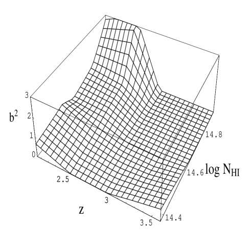
Figure 7: The bias function $b_{{\rm{Ly}\alpha}}^{2}(z,N_{HI})$, assuming $\Omega_{0}=1$.

In Fig. 6 we show the clustering trend in the six subsets of Table 2, for $\log N_{HI}\geq 13.8$, assuming $\Omega_{0}=1$. The clustering increases regularly from $z\simeq 3.5$ to $z\simeq 2$, although the increase is considerably faster at low $z$. Assuming as a reference the CDM predictions with $\Gamma=0.2$ and linear evolution, we can estimate from the sets in Table 2 the biasing function

$$b_{{\rm Ly}\alpha}^{2}(z,N_{HI}) = {\rho_{n}(z,<N_{HI}>)-1\over\rho_{n,CDM}(z)-1}=$$ (17)

$$P_{{\rm Ly}\alpha}(k)/P_{cdm}(k)$$

which expresses for any given average $<N_{HI}>$ and any given redshift, the relation between the real clustering and the linear CDM predicted clustering (the average $<N_{HI}>$ has been obtained excluding the very few lines with $\log H_{HI}>16$). Clearly, $b_{{\rm{Ly}\alpha}}\geq 1$ means that the data are more clustered than the linear-extrapolated CDM distribution; $b_{Ly\alpha}\leq 1$ implies an under-clustering of the data. In Fig. 7 we plot the function $b_{{\rm{Ly}\alpha}}^{2}(z,N_{HI})$. As already mentioned, the real evolution is likely to be both in column density and clustering strength. If one assumes arbitrarily that the average column density does not change with time, then the evolution in redshift turns out to be extremely fast. In flat space, clustering growth as fast as $(1+z)^{-3}$ or faster seem to fit the trend we obtain for high column density cut-offs. One can obtain more reasonable values, i.e. values of closer to the linear trend only by assuming at the same time a decrease of the average column density with decreasing redshift. To give a rough approximation, mostly valid at redshift near 2, we can fit the function $b_{{\rm{Ly}\alpha}}$ as

$$b_{{\rm{Ly}\alpha}}=\left(\frac{N_{HI}}{N_{1}}\right)^{0.65}\left(\frac{1+z}{1+z_{1}}\right)^{-1.7}$$ (18)

where $z_{1}$=3, and $N_{1}=7.1\cdot 10^{14}$ atoms/cm² if $\Omega_{0}=1$, and as

$$b_{{\rm{Ly}\alpha}}=\left(\frac{N_{HI}}{N_{1}}\right)^{0.6}\left(\frac{1+z}{1+z_{1}}\right)^{-1.4}$$ (19)

where $z_{1}$ is the same, and $N_{1}=9.7\cdot 10^{14}$ atoms/cm² for $\Omega_{0}=0.4$. The relative error in the exponents is in all cases of the order of 30%. The bias function shows quantitatively the clustering trend both in column density and redshift. As an interesting consequence, we see that the clustering evolves linearly, i.e. $b_{{\rm{Ly}\alpha}}$ is constant in redshift, only if $N_{HI}\sim(1+z)^{1.7/0.65}\sim(1+z)^{2.6\pm 1}.$ (or as $(1+z)^{2.3\pm 1}$ for the open case). Notice that this conclusion is independent of the overall amplitude of the bias function; it depends only on the relative level of clustering of the Ly$\alpha$ distributions.

Two caveats have to be kept in mind. First, our assumption of a scale-independent bias may prove incorrect. However, we used it as a simple way to parameterize the Lyman-$\alpha$ spectrum in terms of the CDM spectrum, and as such it looks, a posteriori, as an acceptable approximation. Second, the clustering evolution of the clouds need not be linear, even at the scales we are investigating. In fact, along with the linear evolution due to the gravitational instability, the clustering may evolve also in response to the evolution of the ionising sources. If, as shown e.g. by Bagla (1998), the evolution of the clustering of the first collapsed objects is far from linear at $z>1$, then the Lyman-$\alpha$ clouds evolution could also be non-linear.

6 Conclusions

The aim of this paper was to reconstruct the power spectrum of the Lyman-$\alpha$ clouds as a function both of redshift and average column density, and to compare it to theoretical CDM models. We first estimated directly the line-of-sight power spectrum: we concluded that there is no evidence of characteristic scales in the cloud distribution, contrary to what is found in some galaxy surveys. Since the direct reconstruction of the power spectrum is too noisy to derive useful comparisons with theoretical expectations, we employed next the integrated density of neighbours. We assumed that the cloud spectrum can be fitted by

$$P_{{\rm Ly}\alpha}(z,k)=b_{{\rm Ly}\alpha}^{2}(z,N_{HI})P_{cdm}(z,k)$$ (20)

where $b_{{\rm Ly}\alpha}^{2}$ characterizes the Lyman-$\alpha$ line bias with respect to a CDM model normalized to the cluster abundance. This fit performs acceptably well for scales between 1 and 10 Mpc$/h$, while the data are systematically anticorrelated on larger scales. We found that the Ly$\alpha$ clouds are clustered with power similar to the theoretical CDM only at redshift near 2 and average column density higher than 10^13.3 HI atoms/cm², being underclustered ($b_{{\rm Ly}\alpha}^{2}<1$) in all the other cases. A reasonable expectation is that the cloud evolution is linear for most of the scales considered here. Imposing this condition upon the fits (18) and (19) we conclude that the average column density must decrease in time as $N_{HI}\sim(1+z)^{2.6}$ (or as $(1+z)^{2.3}$ for a $\Omega_{0}=0.4$ universe). For the popular model with a cosmological constant such that $\Omega_{\Lambda}=0.6$ the results of the open case applies to a good approximation, since $\Omega_{\Lambda}$ does not affect significantly the clustering evolution. Notice that the function $b_{{\rm Ly}\alpha}$ depends on assuming the specific parametric form (20) and in particular on the clustering redshift evolution of the dark matter spectrum. However, the trend in $z$ we find is so fast that it seems difficult to account for it without a strong redshift decrease of $N_{HI}$.

It is clear that the dataset investigated here is too small to give definitive results. One of the problems is that the most recent and higher cut-off samples are also the most sparse, and thus give higher statistical uncertainty. One conclusion is however rather firm: the cloud clustering can be explained only by assuming a simultaneous increase in correlation and decrease in average column density with redshift.

References

- [1] Bagla J. S., 1998, MNRAS, 299, 417
- [2] Bi H., Davidsen A. F., 1997, ApJ, 479, 523
- [3] Carbone V., Savaglio S., 1996, MNRAS, 282, 868
- [4] Carswell R. F., Lanzetta K. M., Parnell H. C., Webb J. K., 1991, ApJ, 371, 36
- [5] Chernomordik V.V., 1995, ApJ, 440, 431
- [6] Colless M. M., 1998, Phil. Trans. Roy. Soc. Lond.A, in press, astro-ph/9804079
- [7] Cristiani S., D’Odorico S., Fontana A., Giallongo E., Savaglio S., 1995, MNRAS, 273, 1016
- [8] Cristiani S., D’Odorico S., D’Odorico V., Fontana A., Giallongo E., Savaglio S., 1997, MNRAS, 285, 209
- [9] Croft R., Weinberg D., Katz, N., & Hernquist L., 1998, ApJ, 495, 44
- [10] Crotts A., Fang Y., 1998, ApJ, 502, 16
- [11] Davis M., Efstathiou G., Frenk C., White S.D.M., 1985, ApJ, 292, 371
- [12] Dinshaw N., Impey C. D., Foltz C. B., Weymann R. J., Chafee F. H., 1994, ApJ, 437, L87
- [13] D’Odorico V., Cristiani S., D’Odorico S., Fontana A., Giallongo E., A&AS, 127, 217
- [14] El-Ad H., Piran T. & Da Costa L.N., 1996, ApJ, 462, L13
- [15] El-Ad H., Piran T. & Da Costa L.N., 1997, MNRAS, 287, 790
- [16] Hu E. M., Kim T., Cowie L. L., Songaila A., 1995, AJ, 110, 1526
- [17] Hui L. Gnedin N. Y., Zhang Y., 1997, ApJ, 486, 599
- [18] Khare P., Srianand D. G., York D. G., Green R., Welty D., Huang K.–L., Bechtold J., 1997, MNRAS, 285, 167
- [19] Kim T.–S., Hu E. M., Cowie L. L., Songaila A., 1997, AJ, 114, 1
- [20] Kulkarni V. P., Huang K., Green R. F., Bechtold J., Welty D. E., York D. G., 1996, MNRAS, 279, 197
- [21] Lin H., Kirshner R. P., Shectman S. A., Landy S. D., Oemler A., Tucker D. L., Schechter P. L., 1996, ApJ, 471, 617
- [22] Loveday J., 1996, Proc. XXXIst Rencontres de Moriond, astro-ph/9605028
- [23] Lu L., Sargent W. L. W., Barlow T. A., 1997, ApJ, 484, 131
- [24] Maddox S. J., 1998, in ‘Large Scale Structure: Tracks and Traces’, World Scientific, in press
- [25] Miralda–Escudè J., Cen R., Ostriker J. P., Rauch M., 1996, ApJ, 471, 582
- [26] Padmanabhan T., Structure formation in the universe, Cambridge University Press, 1993.
- [27] Pando J., Fang L.–Z., 1996, ApJ, 459, 1
- [28] Park C., Vogeley M.S., Geller M.J., & Huchra J.P., 1994, ApJ, 431, 569
- [29] Peacock J. A. & Dodds S.J., 1994, MNRAS, 267, 1020
- [30] Peacock J. A. & Dodds S.J., 1996, MNRAS, 280, 19
- [31] Rauch M., Carswell R.,F., Chafee F. H., Foltz C. B., Webb J. K., Weymann R. J., Bechtold J., Green R. F., 1992, ApJ, 390, 387
- [32] Rauch M., Haehnelt M., 1995, MNRAS, 275, L76
- [33] Rauch M., Haehnelt M., Steinmetz M., 1997, ApJ, 481, 601
- [34] Rodríguez-Pascual P.M., De La Fuente A., Sanz J.L., Recondo M.C., Clavel J., Santos-Lleó M., Wamsteker W., 1995, ApJ, 448, 575
- [35] Sargent W. L. W., Young P. J., Boksenberg A., Tytler D., 1980, ApJS, 42, 41
- [36] Savaglio S., Carbone V., 1997, Proc. Sesto Workshop on Dark and Visible Matter in Galaxies, eds. M. Persic and P. Salucci, A.S.P. Conference Series, Vol. 117, p491
- [37] Savaglio S., Cristiani, D’Odorico S., Fontana A., Giallongo, E., Molaro P., 1997, A&A, 318, 347
- [38] Savaglio S., Ferguson H. C., Brown T. M., et al., 1999, ApJ, L5
- [39] Smette A., Robertson J.G., Shaver P.A., Reimers D., Wisotzki L., Köhler Th., 1995, A&AS, 113, 199
- [40] Stocke J.T., Shull M., Penton S., Donahue M., Carilli C., 1995 ApJ, 451,24
- [41] Szomoru A., Guhathakurta P., van Gorkom J.H., Knapen J.H., Weinberg, D.H., & Fruchter A.S., 1994, AJ, 108, 491
- [42] Tadros H. & Efstathiou G., 1995, MNRAS, 282, 1381
- [43] Tadros H. & Efstathiou G., 1996, MNRAS, 285, L5
- [44] Webb J. K., 1987, in Hewett A., Burbidge G., Fang L. Z. eds., Proc. IAU Symp. 124, Observational Cosmology. Reidel, Dordrecht, p. 803
- [45] Weinberg D. H., Miralda–Escudè J., Hernquist L., Katz N., 1997, ApJ, 490, 564
- [46] White S. D. M., Efstathiou G. P., & Frenk C. S., 1993, MNRAS, 262, 1023