CD Tau: a detached eclipsing binary with a solar-mass companion

Abstract

We present a detailed analysis of the detached eclipsing binary CD Tau. A large variety of observational data, in form of IR photometry, CORAVEL radial velocity observations and high-resolution spectra, are combined with the published light curves to derive accurate absolute dimensions and effective temperature of the components, as well as the metal abundance of the system. We obtain: $M_{\rm A}=1.442(16)$ M_⊙, $R_{\rm A}=1.798(17)$ R_⊙, ${T_{\rm eff}}_{\rm A}=6200(50)$ K, $M_{\rm B}=1.368(16)$ M_⊙, $R_{\rm B}=1.584(20)$ R_⊙ and ${T_{\rm eff}}_{\rm B}=6200(50)$ K. The metal content of the system is determined to be $[Fe/H]=+0.08(15)$ dex.

In addition, the eclipsing binary has a K-type close visual companion at about 10-arcsec separation, which is shown to be physically linked, thus sharing a common origin. The effective temperature of the visual companion (${T_{\rm eff}}_{\rm C}=5250(200)$ K) is determined from synthetic spectrum fitting, and its luminosity ($\log L/\mbox{L${}_{\odot}$}=-0.27(6)$), and therefore its radius ($R=0.89(9)$ R_⊙), are obtained from comparison with the apparent magnitude of the eclipsing pair.

The observed fundamental properties of the eclipsing components are compared with the predictions of evolutionary models, and we obtain good agreement for an age of 2.6 Gyr and a chemical composition of $Z=0.026$ and $Y=0.26$. Furthermore, we test the evolutionary models for solar-mass stars and we conclude that the physical properties of the visual companion are very accurately described by the same isochrone that fits the more massive components.

1 Introduction

Double-lined eclipsing binaries are the only objects, apart from the Sun, for which fundamental and simultaneous determinations of masses and radii can be obtained. These determinations are possible through the analysis of spectroscopic data in the form of radial velocity curves, and from modelling the photometric data in light curves. In addition, if we consider detached double-lined eclipsing binaries, no significant mass transfer has occurred between the components, since they are smaller than their respective Roche lobes. In such a case, the mutual interaction can be safely neglected and the components can be assumed to evolve like single, individual stars. Therefore, these objects yield simultaneous absolute dimensions for two single stars that are supposed to have a common origin both in time and chemical composition. In this situation, evolutionary models should be able to predict the same age for both components for a certain chemical composition.

Eclipsing binaries that are members of physically bound multiple systems provide additional constraints for the analysis of evolutionary models. All the information that can be extracted for the companion/s (effective temperature, magnitude difference, mass, …) should be also fitted by the same isochrone that fits the eclipsing binary pair. Not many studies have made use of this possibility up to date, mainly because of the scarce amount of information available for the additional stellar companions.

CD Tau (HD 34335, HIP 24663) is a bright eclipsing binary ($V_{\rm max}=6.75$) composed of two similar F6 V stars, which was suggested by Chambliss (1992) as a possible member of a triple system. It has a K-type close visual companion (CD Tau C) at 9.98 arcsec (ESA 1997) with a magnitude of $V=9.9$. The angular distance between the eclipsing pair (CD Tau AB) and CD Tau C is large enough to allow the possibility of obtaining relevant astrophysical information for all three components separately.

Evolutionary models for stars with $M\ga 1.2$ M_⊙ are known to provide a reasonably good description of the observed stellar properties, at least within the main sequence. The relatively large amount of eclipsing binary and open cluster data in this mass range (Andersen 1991; Pols et al. 1998) has been of remarkable help for reaching such an agreement. Nevertheless, recent studies (Popper 1997; Clausen, Helt & Olsen 1999) have pointed out that current stellar evolutionary models are unable to appropriately describe the observed properties of low-mass eclipsing binaries (0.7–1.1 M_⊙). The authors have found that the models for the less massive stars seem to predict radii that are too small ($\log~{}g$ too large) and effective temperatures that are too high when compared to observational data. Clausen et al. (1999) suggest several possible causes of the discrepancy: observational problems, lack of chemical composition determinations and the inaccuracies of the physics of the models, in particular the mixing length parameter. In any case, the number of systems in this mass range is still very small to reach statistically significant conclusions. CD Tau C, which is apparently a sub-solar mass star, may yield useful information for evolutionary model testing and could also help in the solution of the dilemma indicated by Popper (1997) and Clausen et al. (1999).

In this paper, we give a detailed description of the available observational data on CD Tau and their analysis for the determination of the fundamental properties of the three components. Moreover, the existence of a physical link between CD Tau AB and CD Tau C is proved. We finally compare the resulting parameters with the evolutionary model predictions in order to assess their ability to reproduce the observations.

2 Modelling the radial velocity and light curves

A radial velocity curve of CD Tau was published by Popper (1971), but the quality of the data and the poor phase coverage do not allow an accurate determination of the masses. Therefore, new radial velocity observations were secured with the CORAVEL scanner (Baranne, Mayor & Poncet 1979) attached to the 1-m telescope of the Observatoire de Genève and located in the Observatoire d’Haute Provence (France). Two different observational campaigns (1997 February and October) allowed us to collect 48 and 46 measurements for the primary and secondary components, respectively, and 4 measurements for the visual companion. Heliocentric corrections to both Julian date and radial velocity were applied, and the correlation dips were analysed by considering colour dependence (see Baranne et al. 1979; Duquennoy, Mayor & Halbwachs 1991). The final radial velocity measurements for all components, together with their errors, are listed in Table 1.

Table 1: CORAVEL radial velocity observations of CD Tau A, B and C.

HJD –	$v_{\rm r}$	$\sigma_{v_{\rm r}}$	HJD –	$v_{\rm r}$	$\sigma_{v_{\rm r}}$
2450000	(km s-1)		2450000	(km s-1)
A component
498.285	65.0	1.4	500.414	$-$106.1	1.1
498.305	65.6	1.3	501.281	23.7	1.2
498.316	68.8	1.2	501.289	26.1	1.0
498.332	67.6	1.4	501.309	28.3	1.1
498.344	67.7	1.2	501.316	29.8	1.2
498.355	69.8	1.1	501.340	32.0	1.1
498.371	68.2	1.0	501.352	34.4	1.2
498.387	67.6	1.1	501.441	45.3	1.2
498.398	68.0	1.1	502.270	35.5	1.0
498.414	70.3	1.3	502.277	34.6	1.1
498.434	65.3	1.3	502.305	31.7	1.1
499.367	$-$50.7	1.7	505.262	67.1	1.3
499.379	$-$51.8	1.3	505.270	66.2	1.5
499.395	$-$54.7	1.2	505.289	67.1	1.0
499.414	$-$60.3	2.4	505.305	65.8	1.1
499.434	$-$62.4	1.2	505.363	66.0	1.0
500.273	$-$123.9	1.1	729.576	$-$58.8	1.4
500.281	$-$122.1	1.3	729.588	$-$61.3	1.2
500.293	$-$122.3	1.3	729.595	$-$62.4	1.3
500.320	$-$119.5	1.0	730.587	$-$104.3	1.2
500.332	$-$122.6	1.3	732.678	$-$0.2	1.1
500.336	$-$116.4	1.3	733.631	$-$123.7	1.0
500.391	$-$114.8	1.3	736.626	$-$86.5	1.2
500.402	$-$112.5	1.1	737.627	$-$85.8	1.1
B component
498.293	$-$128.7	1.4	500.422	56.0	1.4
498.312	$-$131.8	1.3	501.273	$-$86.2	1.5
498.324	$-$134.1	1.6	501.285	$-$88.8	1.6
498.340	$-$131.9	1.5	501.312	$-$92.3	1.6
498.352	$-$131.4	1.3	501.320	$-$92.7	1.5
498.359	$-$130.4	1.4	501.344	$-$97.0	1.5
498.379	$-$131.9	1.9	501.355	$-$96.2	1.6
498.391	$-$131.2	1.3	501.449	$-$108.2	1.5
498.406	$-$127.9	1.3	502.266	$-$97.8	1.5
498.426	$-$129.8	1.4	502.273	$-$97.6	1.5
498.441	$-$131.0	1.4	502.281	$-$95.9	1.6
499.371	$-$10.1	2.0	502.301	$-$94.8	1.5
499.387	$-$4.8	1.7	505.266	$-$132.7	1.6
499.402	2.0	1.5	505.270	$-$131.2	1.7
499.426	5.4	1.7	505.281	$-$133.0	1.4
499.441	5.6	1.6	505.297	$-$132.0	1.6
500.277	65.1	1.3	729.581	7.6	1.5
500.285	67.1	1.6	729.602	9.8	1.5
500.297	64.6	2.1	730.601	53.2	1.7
500.328	62.2	1.7	732.682	$-$49.8	1.9
500.336	63.2	1.6	733.635	71.3	1.4
500.340	63.5	1.4	736.620	35.4	1.7
500.398	59.8	1.4	737.627	32.9	1.5
C component
498.297	$-$27.6	1.5	500.346	$-$26.9	1.6
500.289	$-$29.1	1.8	501.289	$-$27.7	1.4
Mean value: $-27.8\pm 0.8$

The solution of a radial velocity curve for a circular orbit, such as that of CD Tau AB, is a conceptually very simple problem. The only free parameters are the two velocity semi-amplitudes ($K_{\rm A}$ and $K_{\rm B}$), the systemic velocity ($\gamma$) and a phase offset. The ephemeris for CD Tau, for both radial velocity and light curve solutions, was adopted as $\mbox{Min I}=2441619.4075+3\aas@@fstack{d}435137\,E$ (Kholopov et al. 1987). We used the SBOP program (created by Dr. P.B. Etzel in 1978 and later revised several times) and adopted the Lehmann-Filhés method (Lehmann-Filhés 1894; Underhill 1966) for simultaneous solution of a double-lined radial velocity curve. The parameters resulting from this analysis are shown in Table 2 and a plot of the observed radial velocities and the best-fitting curve is presented in Fig. 1. The r.m.s. residual of the fit is as small as 0.3 km s^-1. The errors of the parameters were conservatively adopted as twice the standard errors provided by the SBOP program. Our results show good agreement with the analysis of the previously published radial velocity curve of Popper (1971), although the curve coverage and the individual accuracy of the measurements are significantly better in our study, leading to smaller formal errors.

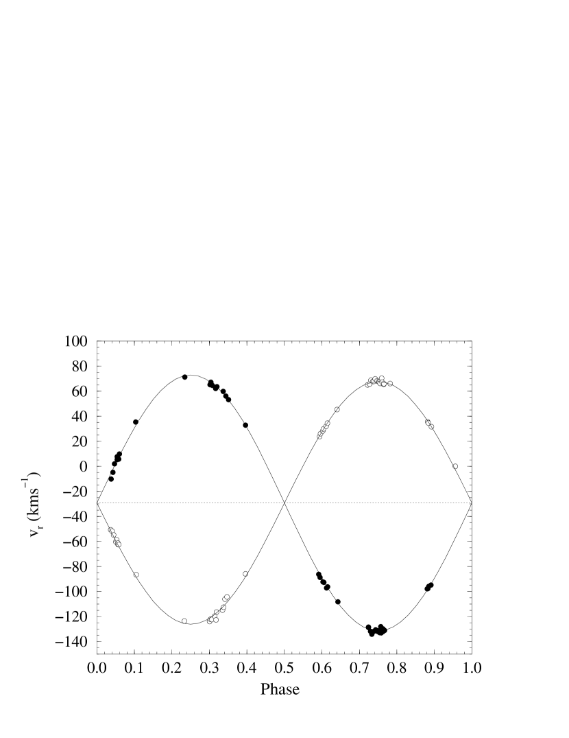
Figure 1: Radial velocity curve fit to CD Tau AB CORAVEL observations from 1997 February and October. Circular orbit is adopted. The r.m.s. residual of the fit is 0.3 km s^-1.

Three complete photoelectric light curves of CD Tau have been observed to our knowledge by Srivastava (1976), Wood (1976) and Gülmen et al. (1980). The best data are those of Wood, obtained in the Strömgren system, but, unfortunately, the individual measurements were not published and are not available. Thus, for this work, we made use of the observations of Gülmen et al. with 292 measurements in each of $B$ and $V$ filters.

The analysis of light curves was done by using an improved version of the Wilson & Devinney (1971, hereafter WD) program (Milone, Stagg & Kurucz 1992; Milone et al. 1994) that includes Kurucz (1991, 1994) ATLAS9 atmosphere models. As suggested by the uncomplicated shape of the light curve (Fig. 2), we chose a detached configuration with coupling between luminosity and temperature when running the solutions. Reflection and proximity effects were considered for the sake of completeness, but their effect is expected to be negligible for such a well-detached system. The bolometric albedos were set to 0.5 (typical for convective atmospheres) and the gravity darkening exponents were adopted as 0.28 and 0.30 (A and B component, repectively) as deduced from the new computations of Claret (1998). The mass ratio $q$ was fixed to the spectroscopic value of 0.948, circular orbit was adopted and the temperature of the primary star was set to 6200 K (see Sect. 3). Finally, both components were assumed to rotate synchronously with the orbital period.

Both $BV$ light curves were solved for simultaneously in order to achieve a single, mutually consistent solution. The free parameters in the light curve fitting were: the phase offset, $\phi_{\circ}$, the inclination, $i$, the temperature of the secondary, $T_{\rm B}$, the gravitational potentials, $\Omega_{\rm A}$ and $\Omega_{\rm B}$, the monochromatic luminosity of the primary, $L_{\rm A}$, and a third light contribution, $F_{3}$.

An automatic procedure was employed to run the WD program. At each iteration, the differential corrections were applied to the input parameters to build the new set of parameters for the next iteration. The result was carefully checked in order to avoid possible unphysical situations (like e.g. Roche lobe filling in detached configuration). A solution was defined as the set of parameters for which the differential corrections suggested by the WD program were smaller than the standard errors during three consecutive iterations. However, when a solution was found, the program did not stop. Instead, it was kept running in order to test the stability of the solutions, to evaluate their scatter and to check for possible spurious solutions. In the case of CD Tau, several runs done from different initial conditions converged to a stable minimum. We finally adopted the parameters that are listed in Table 2.

Table 2: Orbital and stellar parameters for CD Tau A and B derived from the analysis of the light and radial velocity curves, standard photometry and spectroscopy. The numbers in parentheses are the adopted errors affecting the last digits of each parameter.

Radial velocity curve solution
$K_{\rm A}=96.8(5)$ km s-1	$q=\frac{M_{\rm B}}{M_{\rm A}}=0.948(7)$	$\gamma=-29.3(3)$ km s-1
$K_{\rm B}=102.1(5)$ km s-1	$a=13.52(7)$ R⊙
Light curve solution
$P=3.435137^{\rm a}$ days	$e=0^{\rm a}$	$\left.\frac{L_{\rm B}}{L_{\rm A}}\right|_{B}$ = 0.770(22)
$r_{\rm A}$ = 0.1330(10)	$i=87\aas@@fstack{\circ}7(3)$	$\left.\frac{L_{\rm B}}{L_{\rm A}}\right|_{V}$ = 0.772(23)
$r_{\rm B}$ = 0.1172(13)	$\frac{{T_{\rm eff}}_{\rm B}}{{T_{\rm eff}}_{\rm A}}$ = 0.999(1)	$F_{3}|_{B}=0.052(15)^{\rm b}$
		$F_{3}|_{V}=0.066(15)^{\rm b}$
Photometry and spectroscopy
$\overline{T}_{\rm eff}=6200(50)$ K	$[Fe/H]=+0.08(15)$ dex	$E(B-V)=0.0$ mag
${v_{\rm rot}}_{\rm A}=28(3)$ km s-1	${v_{\rm rot}}_{\rm B}=26(3)$ km s-1
Stellar physical properties
$\begin{array}[]{lll}M_{\rm A}=1.442(16)~{}{\rm M}_{\odot}&\mbox{\hskip 56.9055pt}&M_{\rm B}=1.368(16)~{}{\rm M}_{\odot}\\ R_{\rm A}=1.798(17)~{}{\rm R}_{\odot}&&R_{\rm B}=1.584(20)~{}{\rm R}_{\odot}\\ \log g_{\rm A}=4.087(10)~{}{\rm dex}&&\log g_{\rm B}=4.174(12)~{}{\rm dex}\\ {T_{\rm eff}}_{\rm A}=6200(50)~{}{\rm K}&&{T_{\rm eff}}_{\rm B}=6200(50)~{}{\rm K}\end{array}$

^a Adopted, ^b Phase dependent quantity: reference phase = $0\aas@@fstack{p}25$

A especially conflictive parameter is the third light since possible strong correlations with other free parameters may drive us to a wrong solution. The correlation matrix was checked for this possibility and we noticed weak correlations between $F_{3}$ and all the remaining parameters but the inclination, for which the correlation coefficient was close to 0.9. This is a predictable result since the presence of third light affects the relative depths of the eclipses. Actually, the inclusion of $F_{3}$ as a free parameter in the solution of the light curve should only obey to an external evidence of some light excess. For this system, the situation is clear: the photometric observations of Gülmen et al. (1980) included the visual companion inside the diaphragm so that some amount of extra light is certainly present. Since we know that the $V$ magnitude difference is about 3 mag and that the spectral type is later than that of the eclipsing pair components ($\Delta(B-V)\approx 0.4$, from Tycho photometry in the Hipparcos and Tycho catalogues, ESA 1997), we expect an excess of light of about 6.3 per cent in $V$ and 4.4 per cent in $B$. These figures are actually very close to the values derived from the light curve analysis, and the colour behaviour is also reproduced, thus giving additional physical meaning to the best-fitting parameters obtained.

Figure 2: Light curve fit to the observed $B$ and $V$ Comparison$-$Variable (Cp$-$V) differential photometry of CD Tau. Also shown are the Observed$-$Computed (O$-$C) residuals. Solutions obtained with WD program applied to the observations of Gülmen et al. (1980).

The uncertainties in the parameters presented in Table 2 were carefully evaluated by means of two different approaches. On the one hand, the WD program yields the standard error associated to each adjusted parameter. On the other hand, the error can also be estimated as the r.m.s. scatter of all the parameter sets corresponding to the iterations between the first solution and the last iteration (about 100). We shall mention that this is, in general, larger than the r.m.s. scatter of the solutions alone, i.e. those that fulfill the criterion previously described. We conservatively adopted the uncertainty as twice whichever of the two error estimates was the largest. The r.m.s. scatters of the residuals in the light curve fit are 0.011 mag ($n=292$) for both $B$ and $V$. Fig. 2 shows the light curve fit to the observed $B$ and $V$ differential photometry and the corresponding residuals, where no systematic trends are observed.

We shall compare our analysis with that of Wood (1976), Gülmen et al. (1980) and Russo et al. (1981). Regarding the first two works, significant differences exist in the inclination and in the fractional radii. The inclination is 0.8–1^∘ larger in our solution, $r_{\rm A}$ is also 0.010 larger in our case, but $r_{\rm B}$ is about 0.005 smaller, the latter implying a large change in the ratio of radii. However, our computed elements are in very good agreement with those of Russo et al. (1981). They also employed the WD program (although an earlier version) to analyse the light curves, while the other authors used Wood’s model. Thus, the reason for the discrepancy in the solutions is probably related to intrinsic differences of the models. The radii of Wood (1976) and Gülmen et al. (1980) lead to a physically unlikely situation for a detached system, with a secondary component too evolved when compared to the primary ($\log~{}g_{\rm A}\ga\log~{}g_{\rm B}$).

As a brief summary, our final solution shows a system composed of two similar stars of about 1.4 M_⊙ in a moderately evolved stage ($\log~{}g\approx 4.1$), although still in the main sequence. The remarkable point is that the absolute dimensions of the components are known to a precision of about 1 per cent.

3 Effective temperature determination

Table 3: Strömgren (from Hauck & Mermilliod 1998) and IR-band (this work) observations for CD Tau AB. The $JHK$ measurements were taken at quadrature, when full light contribution from both components is present. $n$ is the number of averaged photometric measurements.

$V$	$(b-y)$	$m_{1}$	$c_{1}$	$\beta$	$n$	$T_{\rm eff}$	$E(b-y)$	$\log~{}g$
6.742$\pm$0.007	0.322$\pm$0.003	0.157$\pm$0.003	0.456$\pm$0.003	2.627	4	6200	0.0	3.9
$J$	$H$	$K$	$n$	${T_{\rm eff}}_{J}$	${T_{\rm eff}}_{H}$	${T_{\rm eff}}_{K}$	$[Fe/H]^{\rm a}$	$\log~{}g^{\rm a}$
5.791$\pm$0.007	5.579$\pm$0.008	5.530$\pm$0.006	6	6185	6230	6211	0.08	4.1

^a Adopted.

Strömgren-band and IR-band photometry were used for the determination of the “mean” effective temperature of CD Tau AB. Standard Strömgren indices for CD Tau AB were taken from the catalog of Hauck & Mermilliod (1998) and are shown in Table 3. We adopted the extinction correction calibration of Crawford (1975) and the photometric grids of Napiwotzki (1998), based on Kurucz ATLAS9 atmosphere models. The application of these calibrations indicated a negligible amount of interstellar extinction and yielded a value of 6200 K for the effective temperature, as shown in Table 3.

In order to better constrain the effective temperature determination, several measurements of CD Tau in the IR bands were obtained in the 1 m Carlos Sánchez Telescope (Tenerife, Spain). The observations were made on 1998 February 19 and 24, and April 1 and 3, when the eclipsing component was near quadrature. The reduction of the data and the transformation to the $J$, $H$ and $K$ standard filters was done by using the procedure explained in Masana (1999). The Infra-Red Flux Method (IRFM, Blackwell et al. 1990) was employed to obtain an accurate determination of the effective temperature, by comparing the observed flux distribution with Kurucz ATLAS9 model atmospheres. A $\log~{}g$ of 4.1 and $[Fe/H]=+0.08$ (see Sect. 4) were adopted as input parameters in the analysis, although their influence is almost negligible. The resulting values of the effective temperature obtained at each passband are listed in Table 3.

As it can be seen, the mutual agreement between the three $JHK$ determinations is very good, and they are almost identical to the independent value obtained from Strömgren photometry. Therefore, we can confidently adopt a $\overline{T}_{\rm eff}=6200\pm 50$ K, where the error includes both the variance of the average for all filters and the calibration error of the IRFM method (see Alonso, Arribas & Martínez-Roger 1996).

4 Chemical composition

Two high-resolution spectra (0.15 and 0.12 Å/pix) in different spectral regions were obtained with the aim of determining the atmospheric chemical composition of CD Tau AB. The instrument used was an echelle spectrograph attached to the 74-inch (1.9 m) telescope of Mount Stromlo Observatory (Australia). The spectra were obtained on 1997 October 17 and 19, when the eclipsing component was at phase 0$\aas@@fstack{p}$87 and 0$\aas@@fstack{p}$44, respectively. One of the spectra, with an integration time of 900 s, spans 5730 to 6045 Å (around the Na id line of the interstellar medium), whereas the other one covers the range from 3830 to 4070 Å (including the strong lines of Ca ii K and H) with an integration time of 600 s. The $S/N$ ratio is of the order of 60 and 20, respectively. As a preliminary reduction, the raw images were corrected for bias, dark current and flat field using the standard procedures (see Jordi et al. 1995) and then wavelength calibrated. Radial velocity corrections were applied to refer the wavelength scale to the heliocentric reference frame and, finally, the flux scale was normalized to unity.

The element abundances were determined by fitting of synthetic spectra to our observed spectra. Unfortunately, their $S/N$ ratios (especially for the one around Ca ii lines) are too low to allow a very accurate determination of the chemical composition (see Cayrel de Strobel 1985; Edvardsson et al. 1993) but still enough for a preliminary estimation.

For the synthetic spectrum fitting, we adopted Kurucz ATLAS9 models and the set of programs developed by Dr. I. Hubeny (synspec, rotin and synplot). Nevertheless, we modified these programs by considering the double-lined nature of our spectra, in such a way that they use two atmosphere models, two rotational velocities, two turbulent velocities and two radial velocities as input data. The two resulting synthetic spectra are subsequently co-added. Since we are dealing with an eclipsing binary system, the surface gravities and the temperature ratio obtained by modelling the light and radial velocity curves provide us with useful constraints. The “mean” system $\log~{}g$ is 4.1 dex, so we adopted Kurucz atmosphere models at a $\log~{}g$ of 4.0 dex. Nevertheless, several tests with $\log~{}g=4.5$ dex showed a very weak influence of this parameter on the synthetic spectra. The effective temperatures are strongly correlated with the atmospheric chemical composition determination. Thus, it is necessary to adopt accurate and mutually consistent effective temperatures. From the very precise $T_{\rm eff}$ determinations through IR and Strömgren photometry, we adopted atmosphere models computed at $T_{\rm eff}=6200$ K for both components. Since the temperatures are identical, but not the luminosities (i.e. the radii), a factor of 0.77 (see Table 2) was applied to the flux output of the secondary component when co-adding the synthetic spectra.

The radial velocity shifts of each component were computed from the radial velocity curve at the actual phases and introduced as a fixed parameter (42 km s^-1 and $-$103 km s^-1 for the Na id-region spectrum and $-$65 km s^-1 and 8 km s^-1 for the Ca ii-region spectrum). The rotational velocities of each component were initially adopted as the synchronization values, 26 km s^-1 and 23 km s^-1, and were subsequently changed to 28 km s^-1 and 26 km s^-1 in order to obtain the best fit to the line profiles. The error of these rotational velocities is estimated to be about 3 km s^-1.

Taking into account all the adopted input parameters, the spectrum was studied in small intervals 20 Å wide. From several fitting tests at different Fe-peak element abundances ($-$0.1 dex, $-$0.05 dex, 0.0 dex, +0.05 dex, +0.1 dex and +0.15 dex) we deduced that the observed spectrum is best reproduced with a slightly super-solar composition. We estimate a value of $[Fe/H]=+0.08\pm 0.15$ dex. The lack of lines of other elements does not allow abundance determinations, but there exists evidence of a slight underabundance of Na and a slight overabundance of Si, however, with low reliability. The parameters derived from the spectrum analysis are listed in Table 2.

In general, the spectrum covering 5730–6045 Å was found to be of little help to obtain a Fe abundance determination since there are no strong lines of Fe-peak elements, although we obtained a good fit to the stellar Na id line. Moreover, the reddest zone of the spectrum ($\lambda>5970$ Å) was strongly contaminated by non-stellar features.

Figure 3: Fit to an echelle spectrum of CD Tau AB (double-lined, phase = 0$\aas@@fstack{p}$44) from 3910 to 4070 Å obtained at Mt. Stromlo (Australia) on 1997 October 19. The thick line represents the observed spectrum whereas the thin line is the best-fitting synthetic spectrum computed using Kurucz ATLAS9 fluxes. The parameters used for the synthetic spectrum computation as well as some comments to individual features can be found in the text.

The spectrum spanning 3830 to 4070 Å (which is mostly shown in Fig. 3) proved to be much more useful for abundance determination. The wavelength region of $\lambda<3870$ Å showed poor flux detection statistics and it was not used in the fit. The group of Fe, Mg and V lines at $\lambda 3878$ Å were fitted reasonably well, although the blue edge has a slightly different slope. The Balmer line at $\lambda 3889$ Å is somewhat deeper in the synthetic spectrum, but this may be caused by a not very detailed treatment of this broad line in the latter. The lines of Fe-peak elements between $\lambda 3890$ and $\lambda 3910$ Å can be fitted perfectly. However, although the depth of the Fe lines in the 3918–3920 Å region is well reproduced, there seems to be a problem with the continuum level, which shows a dip in the observed spectrum.

The fit to the Ca ii K ($\lambda 3933.7$ Å) and H ($\lambda 3968.5$ Å) line profiles is very good and was useful for determining the rotational velocities along with some strong Fe lines. From the Ca ii H line to $\lambda 4040$ Å the fit to the observed absorption lines is very satisfactory in such a way that the model and the observations are hardly distinguishable in most parts. It is only between $\lambda 4020$ and $\lambda 4028$ Å that a slight underabsorption is present in the observed spectrum, but it seems to be related to some continuum effect. In the remaining zone of the spectrum, we will only point out a couple of features besides the general good agreement. The Fe i line profile at $\lambda 4046$ Å presents a subestimated absorption, especially for the primary component. This behaviour, not observed in any other strong line, appears to be caused by the contribution of another absorption source. This is the strongest Fe i line in this region, and some amount of interstellar absorption at $v_{\rm r}\approx 0$ may be present so that it would be superimposed on the primary component line. The check of such a hypothesis would require the analysis of some spectra of the same region at different phases. Finally, the absorption Fe i feature around $\lambda 4055$ Å is overestimated in the synthetic spectrum while another quite strong Fe i line at $\lambda 4064$ Å is well reproduced.

In conclusion, the agreement between the observed and the synthetic spectrum computed with the parameters listed in Table 2 is good, as shown in Fig. 3. In some features, the slight flux underestimates may be caused by the poor $S/N$ of the observed spectra, by some deficiencies in the synthetic spectra or, more unlikely, in the model atmosphere fluxes.

5 The visual companion: CD Tau C

Radial velocity measurements of CD Tau C were also obtained with the CORAVEL scanner. In spite of the faintness of this star, near the limiting magnitude of the instrument, a very clear correlation dip was present due to the closeness of its spectral type to that of the mask (K2 III). The four measurements lead to a mean $v_{\rm r}=-27.8\pm 0.8$ km s^-1, which should be compared to the systemic velocity of the eclipsing system, $\gamma=-29.3\pm 0.3$ km s^-1, in order to assess the possibility of a physical link. As it is seen, the agreement is fair. Moreover, the magnitude difference between CD Tau AB and CD Tau C is compatible with what is expected for a K-type star located at the same distance as the eclipsing pair.

From Hipparcos measurements, the distance to CD Tau is known to be 73$\pm$9 pc, which means that an angular separation of 9.98 arcsec can be translated into 730 AU. Assuming the total mass of the system to be around 3.7 M_⊙ (0.9 M_⊙ is adopted for CD Tau C) and the current distance to be the semi-major orbital axis, Kepler’s Third Law leads us to an orbital period of $\approx\!10\,000$ yr and a maximum expected radial velocity difference of $\approx\!2.1$ km s^-1. Such a wide system seems not to be capable of surviving any weak encounter with another object. Thus, although it cannot be assured that CD Tau AB and CD Tau C are in orbit around each other, there exist evidences suggesting that they actually form a common pair.

The determination of the largest possible number of parameters for the visual component may be extremely useful when evaluating the model predictions. Unfortunately, neither the precision of the Strömgren photometric indices nor the intrinsic accuracy of the calibrations is enough for a reliable determination of the effective temperature of CD Tau C. Moreover, no IR observations could be collected due to the strong contamination caused by the bright companion. Thus, no reliable temperature estimation was possible from a photometric point of view.

However, an spectroscopic temperature determination of CD Tau C was performed via synthetic spectrum fitting. Along with the spectra of CD Tau AB, two spectra of its faint visual companion were also secured, with identical instrument configurations. The $S/N$ ratios of the spectra were of the order of 4 (the star is about 3 mag fainter), so that any possibility of abundance determination was ruled out. However, since there are strong evidences that CD Tau AB and CD Tau C are a physical system, we can reasonably assume that they share the same chemical composition. Thus, the spectra can provide a valuable estimation of the effective temperature of this early K-type star, for which there is no other clue.

The spectrum fitting was performed in a similar way as for CD Tau AB, but taking into account the single nature of the star. The surface gravity was adopted as 4.5 dex, the radial velocity as $-28$ km s^-1 (from CORAVEL observations) and the same chemical composition as CD Tau AB. Synthetic spectra were computed from Kurucz models at 250 K intervals between 4750 K and 5500 K and compared to the observed spectrum. In many zones, the choice of the best-fitting temperature was not clear due to the noise, but there were two regions (around Ca II H line, which shows some chromospheric emission, and around $\lambda 4045$ Å, with a strong Fe I line) that allowed us to adopt 5250 K as the effective temperature that yields the best fit. The error of this determination is estimated to be around 200 K.

Further information can be extracted from the magnitude difference between the eclipsing pair and the visual component. In the Hipparcos catalogue, the following values of the $Hp$ magnitude are listed for CD Tau AB and CD Tau C:

$$Hp_{\rm AB}=6.871\pm 0.007\hskip 42.67912ptHp_{\rm C}=9.932\pm 0.110$$

that lead to a magnitude difference $\Delta Hp=Hp_{\rm C}-Hp_{\rm AB}=3.06\pm 0.12$ mag. From $\Delta Hp$ we derive:

$$\Delta M_{\rm bol}=\Delta Hp+\Delta BC(Hp)$$

where $BC(Hp)$ is the bolometric correction for the $Hp$ passband. Straightforward transformations lead to:

$$\Delta\log(\frac{L}{\mbox{L${}_{\odot}$}})=-\frac{\Delta Hp+\Delta BC(Hp)}{2.5}$$

From the BC calibration of Cayrel et al. (1997) we adopted $BC(Hp)_{\rm AB}=-0.15\pm 0.05$ and $BC(Hp)_{\rm C}=-0.35\pm 0.05$, leading to a $\Delta BC(Hp)=-0.20\pm 0.07$. These values and their estimated errors can be combined to derive $\Delta\log(L/\mbox{L${}_{\odot}$})=-1.14\pm 0.06$.

The absolute luminosities of CD Tau A and B can be computed from their radii and effective temperatures and we obtain:

$$\log(L/\mbox{L${}_{\odot}$})_{\rm A}=0.63\pm 0.02\hskip 14.22636pt\log(L/\mbox{L${}_{\odot}$})_{\rm B}=0.52\pm 0.02$$

that can be combined to compute the total luminosity of the eclipsing pair, which comes out to be $\log(L_{\rm AB}/\mbox{L${}_{\odot}$})=0.87\pm 0.02$. We finally obtain the luminosity of CD Tau C that is:

$$\log(L_{\rm C}/\mbox{L${}_{\odot}$})=-0.27\pm 0.06$$

Also, from the effective temperature and the luminosity, the radius can be easily computed and we derive $R_{\rm C}=0.89\pm 0.09$ R_⊙. All these values are also in agreement with the results obtained when adopting the magnitude difference listed in Wood (1976).

For illustrative purposes, we present in Fig. 4 an H-R diagram showing the position of CD Tau C and a sample of well-studied eclipsing binaries in the mass range $0.75<(M/\mbox{M${}_{\odot}$})<1.25$, taken from the compilation of Clausen et al. (1999). As it can be seen, CD Tau C is located within the distribution described by all the eclipsing binary components.

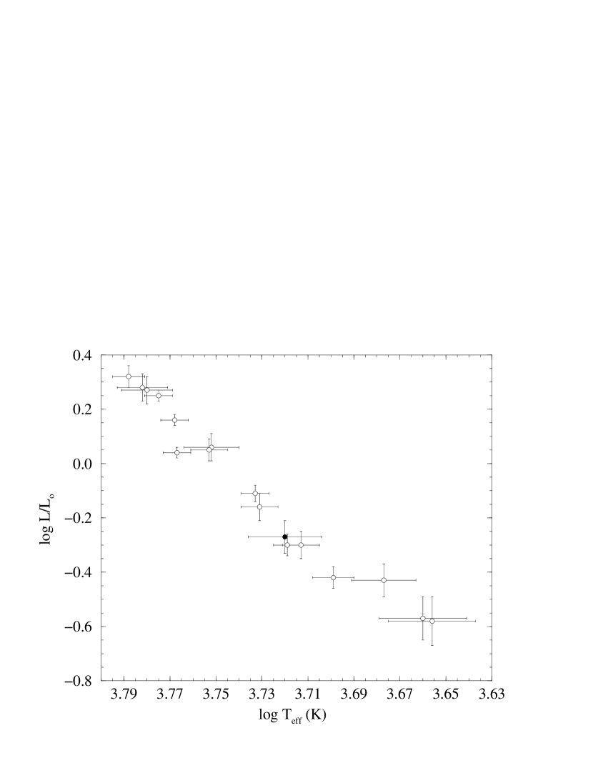
Figure 4: H-R diagram of stars with masses comprised between 0.75 and 1.25 M_⊙. Empty symbols are primary and secondary components of eclipsing binaries, whereas the filled symbol represents CD Tau C.

6 Comparison with evolutionary model predictions

The comparison of model predictions and the observed properties of CD Tau AB was done under the assumption that the evolutionary models should be able to fit an isochrone to both components of the system for a certain chemical composition. We made use of the evolutionary models of CG (Claret 1995, 1997; Claret & Giménez 1995, 1998) that constitute a grid with several $(Z,Y)$ values. The actual isochrone fitting was done by means of an interpolation routine that uses the masses, radii and effective temperature of the components and yields the best-fitting values for the age and the chemical composition $(Z,Y)$ of the system (among other parameters). Thus, both $Z$ (initial metallicity) and $Y$ (initial helium abundance) were treated as free parameters. The computational details of this algorithm will be provided in a forthcoming paper (Ribas et al. 1999).

The evolutionary models predict an age of $2.6\pm 0.3$ Gyr and best-fitting chemical composition values of $Z=0.026\pm 0.007$ and $Y=0.26\pm 0.04$. Indeed, the metal abundance derived from the isochrone fitting is in good agreement with the spectroscopic metallicity determination: $[Fe/H]=+0.08\pm 0.15$ or $Z=0.023\pm 0.008$. A $\log~{}g-\log~{}T_{\rm eff}$ representation of CD Tau A and B, together with the evolutionary tracks and isochrone computed for the best-fitting chemical composition, is presented in Fig. 5.

Figure 5: $\log~{}g-\log~{}T_{\rm eff}$ representation of evolutionary tracks and isochrone for CD Tau A and B. They are computed for the best-fitting value of the chemical composition by using the evolutionary models of CG (see text for references).

Considering the physical relation between CD Tau AB and CD Tau C, a common origin, both in time and composition, can be assumed. This implies that the same isochrone should simultaneously fit all three stars at an age of about 2.6 Gyr. Due to the presumably large mass difference between the components, it is advisable to correct this estimated age by taking into account the different lifetime of the stars in the pre-main sequence (PMS) phase. The evolutionary tracks published by D’Antona & Mazzitelli (1994) indicate that the difference in duration of the PMS phase (the mass of CD Tau C is supposed to be 0.8-0.9 M_⊙) is about 0.1 Gyr. So, the age of CD Tau C has to be corrected to a value of 2.5 Gyr when comparing to post-ZAMS evolutionary models.

In order to compare the observed data with the model predictions, evolutionary tracks of initial masses 0.8, 0.85, 0.9, 0.95 and 1.0 M_⊙ for the adopted chemical composition were kindly provided by Dr. A. Claret. They were computed with the same input physics of the CG evolutionary models. A $\log~{}T_{\rm eff}-\log L$ plot of the evolutionary tracks and the observed values for CD Tau C is presented in Fig. 6. A 2.5 Gyr isochrone is also plotted. As it can be seen, the theoretical predictions and the observational data show an excellent agreement, well within the error bars. Notice that no free parameters remain, since the chemical composition of the star is also known. The best-fitting parameters that the models predict for an age of 2.5 Gyr are a mass of about $M=0.99$ M_⊙ and a $\log~{}g$ of $4.54$ dex.

Figure 6: H-R diagram showing the position of CD Tau C and evolutionary tracks for initial masses from 0.8 to 1.0 M_⊙. A 2.5 Gyr isochrone (the age of CD Tau C) is also shown in the plot. The chemical composition was fixed at $Z=0.026$ and $Y=0.26$.

Further refinement of the effective temperature of CD Tau C (by means of e.g. high-accuracy IR measurements of the visual component alone) may provide a more stringent test to the quality of the evolutionary models. What seems clear at this point, is that the systematics that Popper (1997) and Clausen et al. (1999) pointed out are not observed in CD Tau C. Indeed, the stellar parameters are very accurately described by the isochrone that fits the more massive components.

References

- [1] Alonso A., Arribas S., Martínez-Roger C., 1996, A&AS, 117, 227
- [2] Andersen J., 1991, A&AR, 3, 91
- [3] Baranne A., Mayor M., Poncet J.L., 1979, Vistas in Astronomy, 23, 279
- [4] Blackwell D.E., Petford A.D., Haddock D.J., Arribas S., Selby M.J., 1990, A&A, 232, 396
- [5] Cayrel R., Castelli F., Katz D., Van’t Veer C., Gómez A., Perrin M.-N., 1997, in Battrick B., ed., Hipparcos Venice 1997. ESA SP-402, p. 433
- [6] Cayrel de Strobel G., 1985, in Calibration of fundamental stellar quantities. D. Reidel Publishing Co., Dordrecht, p. 137
- [7] Chambliss C.R., 1992, PASP, 104, 663
- [8] Clausen J.V., Helt B.E., Olsen E.H., 1999, in Giménez A., Guinan E.F., Montesinos B., eds., Theory and Tests of Convection in Stellar Structure. ASP Conference Series, Vol. 173, in press
- [9] Claret A., 1995, A&AS, 109, 441
- [10] Claret A., 1997, A&AS, 125, 439
- [11] Claret A., 1998, A&AS, 131, 395
- [12] Claret A., Giménez A., 1995, A&AS, 114, 549
- [13] Claret A., Giménez A., 1998, A&AS, 133, 123
- [14] Crawford D.L., 1975, AJ, 80, 955
- [15] D’Antona F., Mazzitelli I., 1994, ApJS, 90, 467
- [16] Duquennoy A., Mayor M., Halbwachs J.-L., 1991, A&AS, 88, 281
- [17] Edvardsson B., Andersen J., Gustafsson B., Lambert D.L., Nissen P.E., Tomkin J., 1993, A&A, 275, 101
- [18] ESA 1997, The Hipparcos and Tycho Catalogues, ESA SP-1200
- [19] Gülmen Ö., Ibanoǧlu C., Güdür N., Bozkurt S., 1980, A&AS, 40, 145
- [20] Hauck B., Mermilliod M., 1998, A&AS, 129, 431
- [21] Jordi C., Galadí-Enríquez D., Trullols E., Lahulla F., 1995, A&AS, 114, 489
- [22] Kholopov P.N. et al., 1987, General Catalogue of Variable Stars, 4th. edition. Nauka, Moscow
- [23] Kurucz R.L., 1991, in Crivellari L. et al., eds., Stellar Atmospheres: Beyond Classical Models. Kluwer, Dordrecht, p. 441
- [24] Kurucz R.L., 1994, CD-ROM No 19
- [25] Lehmann-Filhés R., 1894, Astron. Nachr., 163, 17
- [26] Masana E., 1999, PhD thesis, Univ. de Barcelona, in preparation
- [27] Milone E.F., Stagg C.R., Kurucz R.L., 1992, ApJS, 79, 123
- [28] Milone E.F., Stagg C.R., Kallrath J., Kurucz R.L., 1994, BAAS, 184, 06.05
- [29] Napiwotzki R., 1998, private communication
- [30] Pols O.R., Schröder K.-P., Hurley J.R., Tout C.A., Eggleton P.P., 1998, MNRAS, 298, 525
- [31] Popper D.M., 1971, ApJ, 166, 361
- [32] Popper D.M., 1997, AJ, 114, 1195
- [33] Ribas I. et al., 1999, MNRAS, in preparation
- [34] Russo G., Milano L., D’Orsi A., Marcozzi S., 1981, Ap&SS, 79, 359
- [35] Srivastava J.B., 1976, Ap&SS, 40, 15
- [36] Underhill A.B., 1966, The Early Type Stars, p. 127
- [37] Wilson R.E., Devinney E.J., 1971, ApJ, 166, 605 (WD)
- [38] Wood D.B., 1976, AJ, 81, 855