A Measurement of the Angular Power Spectrum of the Microwave Background Made from the High Chilean Andes

Abstract

We report on a measurement of the angular spectrum of the anisotropy of the microwave sky at 30 and 40 GHz between $l=50$ and $l=200$. The data, covering roughly $600\rm\,deg^{2}$, support a rise in the angular spectrum to a maximum with $\delta T_{l}\approx 85~{}\mu$K at $l=200$. We also give a 2-sigma upper limit of $\delta T_{l}<122~{}\mu$K at $l=432$ at 144 GHz. These results come from the first campaign of the Mobile Anisotropy Telescope (MAT) on Cerro Toco, Chile. To assist in assessing the site, we present plots of the fluctuations in atmospheric emission at 30 and 144 GHz.

1. Introduction

The characterization of the CMB anisotropy is essential for understanding the process of cosmic structure formation (e.g. Hu et al. (1997)). If some of the currently popular models prove correct, the anisotropy may be used to strongly constrain cosmological parameters (Jungman et al. (1995), Bond et al. (1998)). Here we report the results from the TOCO97 campaign of the Mobile Anisotropy Telescope (MAT) experiment.

2. Instrument

The MAT telescope is comprised of the QMAP balloon gondola and instrument (Devlin et al. (1998)), mounted on the azimuthal bearing of a surplus Nike Ajax military radar trailer. The receiver has five cooled corrugated feed horns, one at $K_{a}$ band (31 GHz), two at $Q$ band (42 GHz), and two at $D$ band (144 GHz). Each of the $K_{a}$ and $Q$ band horns feed two HEMT-based (high electron mobility transistor) amplifiers (Pospieszalski (1992)) with one in each polarization. The two D band horns each feed a single SIS detector (Kerr et al. (1993)) with one horn in each polarization. This gives a total of eight radiometry channels in the experiment. A Sumitomo mechanical refrigerator cools the HEMT amplifiers to 35 K and the SIS receivers to 4 K.

The telescope optics are similar to those used for three ground-based observing campaigns in Saskatoon, SK (Wollack et al. (1997), SK). The feeds underilluminate an ambient temperature 0.85 m off-axis parabolic reflector which in turn underilluminates a computer controlled 1.8 m$\times$1.2 m resonant chopping flat mirror. The beams are scanned horizontally across the sky in a $\approx 4.6$ Hz sinusoidal pattern. The outputs of the detectors are AC coupled at 0.15 Hz and sampled $N_{c}$ times during each chopper cycle ($N_{c}=80$ for $K_{a}$ and $Q$ bands, and $N_{c}=320$ for $D$ band). The telescope is inside an aluminum ground screen which is fixed with respect to the receiver and parabola.

The telescope pointing (Table 1) is established through observations of Jupiter and is monitored with two redundant encoders on both the azimuth bearing and on the chopper. The absolute errors in azimuth and elevation are 0$\fdg$04, and the relative errors are $<$0$\fdg$01. The chopper position is sampled 80 times per chop. When its rms position over one cycle deviates by more than 0$\fdg$015 from the average position (due to wind, etc.), we reject the data.

Table 1. TOCO97 beam characteristics

Feed	Az	El	$\Omega_{meas}$	$\theta^{FWHM}_{avg}$
	deg	deg	$10^{-4}~{}$sr	deg
$K_{a}$1/2	203.13	41.75	2.75	0.90
$Q$1/2	206.75	41.85	1.69	0.70
$Q$3/4	206.70	39.25	1.77	0.72
$D$1	205.00	40.44	0.183	0.23

3. Observations and Calibration

Figure 1.— The rms detector output in antenna temperature of the $K_{a}$2 and $D$1 channels averaged over 0.68 ms (with the chopper running at the nominal amplitude) vs. day of year in 1997. The sky is most stable between 10 PM and 10 AM local time. Similar results from 1998 are consistent with the NRAO opacity measurements (http://www.tuc.nrao.edu/mma/sites/sites.html).

Data were taken at a 5200 m site on the side of Cerro Toco (lat. = -22$\fdg$95 long. = 67$\fdg$775 ), near San Pedro de Atacama, Chile, from Oct. 20, 1997 to Dec 15, 1997. The receiver was operational 90% of the available time. For the anisotropy data, the primary optical axis is fixed at az = 204$\fdg$9, el = 40$\fdg$5, $\delta$ = -62$\fdg$6 and the chopper scans with an azimuthal amplitude of $2\fdg 96$ (8$\fdg$93 on the sky) as the sky rotates through the beam. The telescope position was not wobbled to the other side of the South Celestial Pole as for the SK measurements in the North. The rms outputs of the $K_{a}$2 and $D$1 channels are shown in Fig. 1.

Jupiter is used to calibrate all channels and map the beams. Its brightness temperature is 152, 160, 170 K for $K_{a}$ through $D$ bands respectively (Griffin et al. (1986), Ulich et al. (1981)), with an intrinsic calibration error of $\approx 5\%$. We account for the variation in angular diameter. We also observe Jupiter with multiple relative azimuthal offsets to verify the chopper calibration.

The uncertainty in the beam solid angle for the $K_{a}$ and $Q$ bands is $\approx 5\%$ as determined from the standard deviation of beam measurements for the MAT and QMAP experiments. From a global fit of the clear-weather Jupiter calibrations, the standard deviation in the fitted amplitudes is 6%. These sources of calibration error dominate the error from the uncertainty in the passband. The total $1\sigma$ calibration error is obtained by combining the intrinsic, beam, and measurement errors in quadrature resulting in 10%, 10%, and 11% in $K_{a}$ through $D$ respectively.

A thermally-stabilized noise source at $T_{\rm eff}\approx 1$ K is switched on twice for 40 msec every 100 seconds as a relative calibration. The pulse height is correlated to the Jupiter calibrations in the $K_{a}$ and $Q$ channels. The variation in detector gain corrected for with these calibration pulses is roughly 5%. No such correction was made for $D$ band.

4. Data Reduction

The reduction is similar to that of the SK experiment (Netterfield et al. (1997)). The raw data, $d_{i}$, are multiplied by “n-pt” synthesis vectors, $SV_{n,i}$ (where $i$ ranges from 1 to $N_{c}$) to yield the effective temperature corresponding to a multilobed beam on the sky, $H(\Omega)$. For example, we refer to the classic three-lobed beam produced by a “double difference” as the “3-pt harmonic” and write $t_{3}=\sum_{i=1}^{N_{c}}SV_{3,i}d_{i}$. We also generate the quadrature signal $q_{n}$ (data with chopper sweeping in one direction minus that with the sweeping in the other direction) and fast-dither signal $f^{d}_{n}$ (one value of $t_{n}$ minus the subsequent one). For both $K_{a}$1/2 and $Q$3/4 we analyze the unpolarized weighted mean of the combined detector outputs.

The phase of the data relative to the beam position is determined with both Jupiter and observations of the galaxy. We know we are properly phased when the quadrature signal from the galaxy is zero for all harmonics.

The harmonics are binned according to the right ascension at the center of the chopper sweep. The number of bins depends on the band and harmonic (Table 2). For each night, we compute the mean and variance of all the $t_{n}$, $q_{n}$, and $f^{d}_{n}$ corresponding to a bin. These numbers are appropriately averaged over the campaign and used in the likelihood analysis.

From the raw dataset of 814250 5s averages, we filter out time spent on instrument calibration (6%), celestial calibrations (11%), observations of the galaxy & daytime (53%), and bad pointing (4%). Accounting for overlap, these cut a total of 57%. The data span RA = $0^{\circ}$ to $140^{\circ}$ ($b=-55^{\circ}$ to $-10^{\circ}$).

The data are selected according to the weather by examining each harmonic independently. We first flag 5s averages with a large rms. The unflagged data are divided up into 15 minute sections and the rms of the $t_{n}$ found. For 15 m sections with rms $>2\sigma$, the constituent 5s averages are not used, as well as those of the preceding and succeeding 15 m sections. We ensure that the cut does not bias the statistical weight. As a final cut, nights with less than 4.7 hours of data are excluded. Repeating the analysis with increased cut values produces statistically similar (within 1$\sigma$) results. The atmosphere cut selects roughly the same sections for $K_{a}$ and $Q$. In the analyses, we discard the 2 and 3-pt data as it is corrupted by atmospheric fluctuations and variable instrumental offsets. If the 4-pt is corrupted, it is at the $1\sigma$ level and not readily detectable.

The stability of the instrument is assessed through internal consistency checks and with the distribution of the offset of each harmonic. The offset is the average of a night of data after the cuts have been applied (ranges from 5-10 hours) and is of magnitude $\approx 200~{}\mu$K with error $20~{}\mu$K. In general, the offset remains constant for a few nights and then jumps 3-5 sigma. The resulting $\chi^{2}/\nu$ is typically between 4 and 20 for the data over the full campaign and is $\approx 1$ for the quadrature signal. In general, a change in offset can have any time scale. The $q_{n}$ and $f^{d}_{n}$ are sensitive to $\tau=0.25~{}$s. We also monitor a slow dither (difference of the subsequent 5 sec averages) with $\tau=5$ s and a night-to-night dither with $\tau=24~{}$h. For the final analysis, we delete one seven day section that has a large jump in offset. To eliminate the potential effect of slow variations in offset, we remove the slope and mean for each night. This is accounted for in the quoted result (both the constraint matrix method, Bond et al. 1998b , and marginalization, Bond et al. (1991) give similar corrections) and does not significantly alter the results over the subtraction of a simple mean. As a test, we have also tried removing quadratic and cubic terms from the offset, with no significant changes in the answer. In summary, there is no evidence that the small instability in the offset affects our results.

We examined the variations in the power spectrum of the synchronously co-added raw HEMT data, and found no evidence for microphonics. However, a microphonic coupling to the SIS detector was exacerbated after situating the telescope at the site. After filtering, residual signals persisted in the quadrature channels (though not in the fast and slow dithers) and so we report only 95% upper limits for the D channel, specifically $\delta T_{l}<180~{}\mu$K at $\ell=325$ and $\delta T_{l}<122~{}\mu$K at $\ell=432$.

The primary effect of data editing is to increase the error bar per point and decrease the upper limits of the null tests. Of the 169 null tests (Table 2 plus fast, slow, and night dithers), there are only three failures. The distribution of the reduced $\chi^{2}$ of the null tests is consistent with noise and inconsistent with any signal. When the data are combined into groups of harmonics and bands, all null tests are consistent with noise.

5. Analysis and Discussion

The analysis of the individual harmonics, because the windows are so narrow, essentially corresponds to finding $\delta T_{l}^{\prime}=\sqrt{(\Delta^{2}_{tot}-\Delta^{2}_{inst})/I(W)}$, where $\Delta^{2}_{tot}$ is the variance of the data for each harmonic, $\Delta^{2}_{inst}$ is the variance due to atmospheric and instrumental noise, and $I(W)=\sum W_{l}/l$. $W_{l}$ is the window function, as defined in Bond (1996). The full likelihood analysis provides a formal way of determining $\delta T_{l}$ that includes correlations and gives the correct error bar in the low signal-to-noise limit.

The error in $I(W)$ is determined from the scatter in the beam values. We find $\delta I(W)/I(W)\lesssim 0.01$ for all bands and harmonics. The mean variance, $\Delta^{2}_{inst}$, is determined directly from the uncertainties in each bin. If these uncertainties are somehow biased, the results of the simple test and full likelihood will be biased. We examine the distribution of all the data for each harmonic from all the nights after removing the mean value of each sky bin. The width of this distribution agrees with the mean error bar indicating that the error per point is not biased. Also, the ratio of the error bars between harmonics agrees with the analytic calculation.

In the full analysis (Fig. 2), we include all known correlations inherent in the observing strategy. From the data, we determine the correlations between harmonics due to the atmosphere, detector noise, and non-orthogonality of the synthesis vectors. The correlation coefficients between bands due to the atmosphere are of order $0.05$. We also examine the autocorrelation function of the data for a single harmonic to ensure that atmospheric fluctuations do not correlate one bin to the next. The quoted results are insensitive to the precise values of the off-diagonal terms of the covariance matrix.

FIG. 2.— Combined analysis of data in Table 2. The values are ($l,\delta T_{l}~{}[\mu{\rm K}]$) $=$ ($63^{+18}_{-18},40^{+10}_{-9}$), ($86^{+16}_{-22},45^{+7}_{-6}$), ($114^{+20}_{-24},70^{+6}_{-6}$), ($158^{+22}_{-23},89^{+7}_{-7}$), ($199^{+38}_{-29},85^{+8}_{-8}$). Error bars are “$1\sigma$ statistical”; calibration error is not included. The COBE/DMR points are from Tegmark (1997). The solid curve is standard CDM ($\Omega_{b}=0.05$, $h=0.5$).

These results are similar to previous results obtained with this technique (SK) though the experiment was done with different optics, a different receiver, a different primary calibrator, largely different analysis code, and observed a different part of the sky. Though we have not correlated our data with templates of foreground emission, the foreground contribution is known to be small at these frequencies and galactic latitudes (Coble et al. (1999), de Oliveira-Costa et al. (1997)). In addition we have examined the frequency spectrum of the fluctuations in $K_{a}$ and $Q$ bands, and find it to be consistent with a thermal CMB spectrum, and inconsistent with various foregrounds. Finally, the full analysis has been repeated after deleting each 15° section of data in RA, indicating that the signal does not arise from one region. (Our scan passes near, but misses, the LMC.) Future work will address the precise level of contamination.

Table 2TOCO97 Angular Spectrum

Band/$SV$	$\ell_{\hbox{eff}}$	$\delta T_{\ell}$	$N_{bins}$	$\delta T_{\ell}^{\prime}$	$\Delta_{tot}$	$\Delta_{inst}$	$\sqrt{I(W)}$	(A-B)/2	Quad, qn	(H1-H2)/2
		$\mu$K		$\mu$K	$\mu$K	$\mu$K		$\mu$K	$\mu$K	$\mu$K
$K_{a}$1/2
4pt	$63^{+17}_{-18}$	$35^{+13}_{-9}$	48(16)	32	33	20	0.84	$<27(0.94)$	$<30(1.05)$	$<29(0.95)$
5pt	$86^{+16}_{-21}$	$52^{+11}_{-8}$	64(28)	49	40	21	0.71	$<21(0.59)$	$<32(1.23)$	$<29(1.05)$
6pt	$107^{+16}_{-21}$	$71^{+12}_{-10}$	96(42)	69	52	27	0.65	$<32(0.90)$	$<31(0.96)$	$<35(1.04)$
7pt	$127^{+16}_{-22}$	$93^{+15}_{-14}$	96(41)	90	57	27	0.55	$<35(0.80)$	$<37(0.90)$	$<30(0.68)$
8pt	$145^{+18}_{-20}$	$103^{+15}_{-13}$	128(55)	102	63	34	0.52	$<51(0.97)$	$<46(1.00)$	$<43(0.91)$
9pt	$165^{+18}_{-20}$	$65^{+16}_{-17}$	128(54)	59	47	38	0.46	$<63(0.95)$	$<72(1.19)$	$<66(1.07)$
10pt	$182^{+21}_{-17}$	$67^{+20}_{-23}$	192(82)	70	60	51	0.44	$<68(0.85)$	$<69(0.94)$	$<60(0.89)$
11pt	$192^{+30}_{-8}$	$<119$	192(82)	67	65	58	0.42	$<91(0.94)$	$<83(1.00)$	$<86(0.96)$
12pt	$215^{+27}_{-11}$	$128^{+30}_{-33}$	192(82)	127	83	68	0.37	$<150(1.11)$	$<86(0.79)$	$<76(0.67)$
$Q$1
4pt	$63^{+17}_{-18}$	$57^{+18}_{-13}$	48(20)	51	53	31	0.83	$\cdots$	$<44(1.04)$	$<47(1.11)$
5pt	$87^{+16}_{-22}$	$40^{+14}_{-14}$	64(28)	34	40	33	0.71	$\cdots$	$<36(0.75)$	$<47(1.09)$
6pt	$110^{+15}_{-24}$	$56^{+14}_{-13}$	96(42)	52	52	40	0.65	$\cdots$	$<45(0.87)$	$52^{+15}_{-14}(1.71)$
7pt	$131^{+14}_{-25}$	$81^{+19}_{-16}$	96(42)	77	59	41	0.55	$\cdots$	$<65(1.12)$	$<53(0.89)$
8pt	$151^{+15}_{-25}$	$86^{+19}_{-17}$	128(55)	79	66	50	0.53	$\cdots$	$<45(0.67)$	$<64(0.89)$
9pt	$172^{+14}_{-26}$	$93^{+23}_{-23}$	128(55)	89	68	54	0.47	$\cdots$	$<82(0.94)$	$<72(0.83)$
10pt	$191^{+16}_{-24}$	$<115$	192(84)	31	75	74	0.47	$\cdots$	$<105(1.13)$	$<92(0.94)$
11pt	$203^{+24}_{-17}$	$<117$	192(84)	44	80	78	0.44	$\cdots$	$<103(0.94)$	$<83(0.81)$
12pt	$221^{+25}_{-15}$	$<169$	192(84)	91	91	84	0.40	$\cdots$	$<138(1.06)$	$<119(0.92)$
13pt	$245^{+21}_{-20}$	$<130$	192(84)	$\cdots$	84	92	0.37	$\cdots$	$<163(1.02)$	$<164(1.06)$
14pt	$267^{+20}_{-23}$	$<202$	256(112)	123	123	114	0.37	$\cdots$	$<183(1.06)$	$<188(1.00)$
$Q$3/4
5pt	$83^{+15}_{-20}$	$47^{+17}_{-13}$	64(17)	43	39	24	0.73	$31^{+10}_{-8}(1.94)$	$<50(1.39)$	$<58(1.73)$
6pt	$106^{+14}_{-23}$	$61^{+18}_{-13}$	96(22)	55	46	28	0.66	$<27(0.68)$	$<34(0.60)$	$<61(1.46)$
7pt	$125^{+14}_{-23}$	$72^{+16}_{-12}$	96(35)	71	50	30	0.56	$<29(0.65)$	$<57(1.30)$	$<31(0.57)$
8pt	$145^{+14}_{-23}$	$115^{+19}_{-15}$	128(45)	109	68	35	0.54	$<26(0.50)$	$<38(0.73)$	$<60(1.18)$
9pt	$165^{+14}_{-24}$	$72^{+24}_{-21}$	128(29)	65	48	37	0.48	$<43(0.82)$	$<97(1.38)$	$<84(1.16)$
10pt	$184^{+15}_{-23}$	$87^{+19}_{-19}$	192(70)	86	63	48	0.47	$<68(1.03)$	$<45(0.78)$	$<52(0.75)$
11pt	$196^{+22}_{-17}$	$90^{+27}_{-26}$	192(54)	84	65	53	0.44	$<64(0.90)$	$<78(0.91)$	$<75(0.78)$
12pt	$212^{+25}_{-13}$	$100^{+29}_{-27}$	192(65)	97	69	57	0.40	$<70(0.95)$	$<129(1.36)$	$<84(0.89)$
13pt	$236^{+20}_{-19}$	$<157$	192(56)	80	71	65	0.37	$<107(1.07)$	$<121(0.93)$	$<153(1.17)$
14pt	$258^{+18}_{-23}$	$119^{+36}_{-38}$	256(103)	119	91	80	0.36	$<116(0.95)$	$<137(1.11)$	$<103(0.78)$

Note. — A “$<$” indicates a 95% confidence limit. Calibration errors are not included. (a) The range for $\ell_{\hbox{eff}}$ denotes the range for which the window function exceeds $e^{-1/2}$ times the peak value. (b) The error on $\delta T_{\ell}=[\ell(\ell+1)C_{\ell}/2\pi]^{1/2}$ is comprised of experimental uncertainty and sample variance. These values are not statistically independent: harmonic numbers differing by 2 are correlated at the 0.35 level. For all harmonics, the sample variance ($\propto 1/\sqrt{2N_{bins}}$) is $\approx 7~{}\mu$K. (c) The number of bins on the sky followed by, in parentheses, the number used in the analysis due to the galactic/atmosphere cut. (d) The reduced $\chi^{2}$ are given in parentheses. (e) $(A-B)/2$ is the difference in polarizations. We have combined bands and harmonics to generate 95% upper limits on polarization, $A-B$, and obtain: ($l,\delta T_{l}~{}[\mu{\rm K}]$) $=$ ($63^{+18}_{-18},<37$), ($86^{+17}_{-21},<54$), ($115^{+21}_{-24},<28$), ($148^{+17}_{-25},<41$), ($195^{+33}_{-23},<79$). (f) $(H1-H2)/2$ is the first half minus the second half.

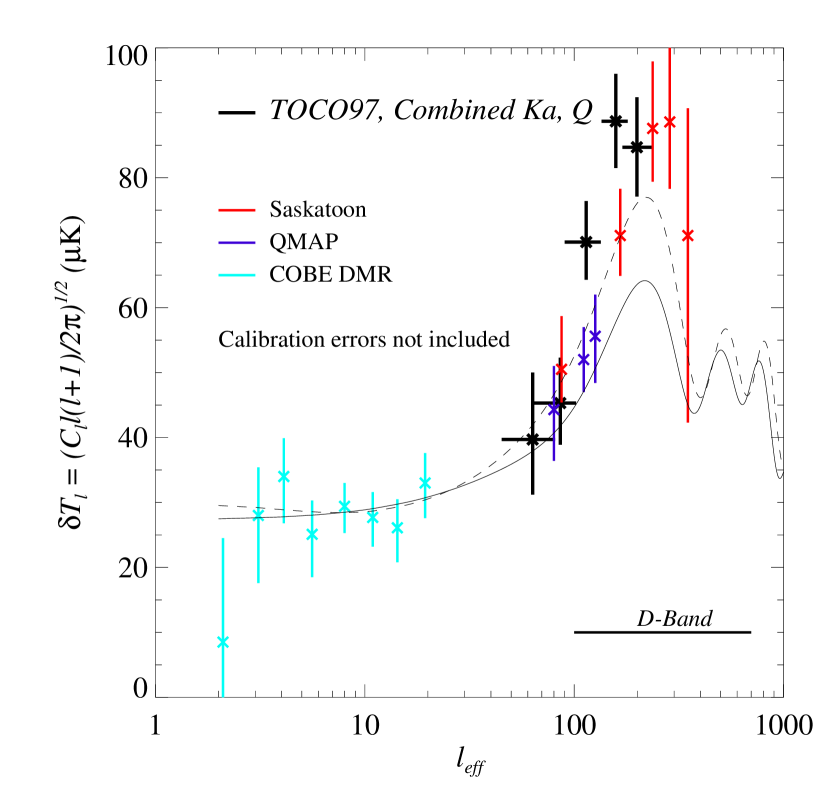
Figure 3.— Angular spectrum from the SK, QMAP, and TOCO97 experiments. The SK data from Netterfield et al. (1997, ApJ, 474:47) and Wollack et al. (1997, ApJ 476:440) have been recalibrated according to the Mason et al. (1997, astro-ph/9903383), leading to an increase of 5%, and reduced according to the forground contribution in de Oliveira-Costa et al. (1997, ApJL, 482:L17), leading to a reduction of 2%. The foreground reduction was applied uniformly. Because the SK data are primarily at 40 GHz, the Mason et al. results must be extrapolated. In addition, uncertainty in the measured passband, measurement uncertainty, and beam uncertainty, must be taken into accounted. This leads to a $1\sigma$ calibration error of 11%. The QMAP data are the same as those reported in de Oliveira-Costa et al. (1998, ApJL, 509:L78) and have an average calibration error of 12%, the correction for foreground emission is $\approx$ 2% (de Oliveira-Costa et al. 1999, in prep), though has not yet been precisely determined and so is not included. Both SK and QMAP are calibrated with respect to Cas-A. The TOCO97 data, which have a calibration error of 10%, are calibrated with respect to Jupiter. A foreground contribution, which is expected to be small, has not been subtracted. When calibration errors are included, all three independent experiments agree. Two cosmological models are shown for reference. The lower is “standard CDM” ($\Omega_{0}=1$, $\Omega_{B}=0.05$, $h=0.5$); the higher one is the current “concordance model” (Bachall et al. 1999 in prep, Turner 1999 astro-ph/9904051) with $\Omega_{0}=0.4$, $\Omega_{B}=0.045$, $\Omega_{\Lambda}=0.6$, and $h=0.65$. For COBE/DMR we use the results from Tegmark.

References

- Bond et al. (1991) Bond, J. R., Efstathiou, G., Lubin, P. M., & Meinhold, P. R. 1991, Phys. Rev. Lett., 66, 2179
- Bond (1996) Bond, J. R. 1996 Theory and Observations of the Cosmic Microwave Background Radiation, in “Cosmology and Large-Scale Structure,” Les Houches Session LX, August 1993, ed. R. Schaeffer, Elsevier Science Press
- Bond et al. (1998) Bond, J. R., Efstathiou, G., & Tegmark, M. 1998, MNRAS, 50, L33
- (4) Bond, J. R., Jaffe, A. H., & Knox, L. 1998, Phys. Rev. D, 57, 2117
- Coble et al. (1999) Coble, K., et al. 1999, astro-ph/9902195
- de Oliveira-Costa et al. (1997) de Oliveira-Costa, A., Kogut, A., Devlin, M. J., Netterfield, C. B., Page, L. A., & Wollack, E. J. 1997 ApJ, 482, L17
- Devlin et al. (1998) Devlin, M. J., de Oliveira-Costa, A., Herbig, T., Miller, A. D., Netterfield, C. B., Page, L., & Tegmark, M. 1998, ApJ, 509, L73
- Griffin et al. (1986) Griffin, M. J., Ade, A. R., Orton, G. S., Robson, E. I., Gear, W.K., Nolt, I. G., & Radostitz, J. V. 1986, Icarus, 65, 244
- Hu et al. (1997) Hu, W., Sugiyama, N., & Silk, J. 1997, Nature, 386, 37
- Jungman et al. (1995) Jungman, G., Kamionkowski, M., Kosowsky, A., & Spergel, D. N. 1995, Phys. Rev. D, 54, 1332
- Netterfield et al. (1997) Netterfield, C. B., Devlin, M. J., Jarosik, N., Page, L., & Wollack, E. J. 1997, ApJ, 474, 47
- Kerr et al. (1993) Kerr, A. R., Pan, S.-K., Lichtenberger, A. W., & Lloyd, F. L. 1993, Proceedings of the Fourth International Symposium on Space Terahertz Technology, 1
- Pospieszalski (1992) Pospieszalski, M. W. 1992, IEEE MTT-S Digest, 1369; also see Pospieszalski, M. W. et al. 1994, IEEE MTT-S Digest, 1345
- Pospieszalski et al. (1997) Pospieszalski, M.W. 1997, Microwave Background Anisotropies (Ed. Frontieres, ed. Bouchet et al.), 23
- Tegmark (1997) Tegmark, M., 1997, Phys. Rev. D, 55, 5895
- Ulich et al. (1981) Ulich, B. L. 1981, AJ, 86, 1619
- Wollack et al. (1997) Wollack, E. J., Devlin, M. J., Jarosik, N.J., Netterfield, C. B., Page, L., & Wilkinson, D. 1997, ApJ, 476, 440