Galaxy Clusters: Oblate or Prolate?

Abstract

It is now well known that a combined analysis of the Sunyaev-Zel’dovich (SZ) effect and the X-ray emission observations can be used to determine the angular diameter distance to galaxy clusters, from which the Hubble constant is derived. Given that the SZ/X-ray Hubble constant is determined through a geometrical description of clusters, the accuracy to which such distance measurements can be made depends on how well one can describe intrinsic cluster shapes. Using the observed X-ray isophotal axial ratio distribution for a sample of galaxy clusters, we discuss intrinsic cluster shapes and, in particular, if clusters can be described by axisymmetric models, such as oblate and prolate ellipsoids. These models are currently favored when determining the SZ/X-ray Hubble constant. We show that the current observational data on the asphericity of galaxy clusters suggest that clusters are more consistent with a prolate rather than an oblate distribution. We address the possibility that clusters are intrinsically triaxial by viewing triaxial ellipsoids at random angles with the intrinsic axial ratios following an isotropic Gaussian distribution. We discuss implications of our results on current attempts at measuring the Hubble constant using galaxy clusters and suggest that an unbiased estimate of the Hubble constant, not fundamentally limited by projection effects, would eventually be possible with the SZ/X-ray method.

1 Introduction

Over the last few years, there has been a tremendous increase in the study of galaxy clusters as cosmological probes, initially through the use of X-ray emission observations, and in recent years, through the use of Sunyaev-Zel’dovich (SZ) effect. Briefly, the SZ effect is a distortion of the cosmic microwave background (CMB) radiation by inverse-Compton scattering of thermal electrons within the hot intracluster medium (Sunyaev & Zel’dovich 1980; see Birkinshaw 1998 for a recent review). The initial motivation for the study of SZ effect was to establish a cosmic origin to the cosmic microwave background (CMB), rather than a galactic one. It was later realized, however, that by combining the SZ intensity change and the X-ray emission observations, and solving for the number density distribution of electrons responsible for both these effects after assuming a certain geometrical shape, angular diameter distance, $D_{\rm A}$, to galaxy clusters can be derived (e.g., Cavaliere et al. 1977; Silk & White 1978; Gunn 1978). Combining the distance measurement with redshift allows a determination of the Hubble constant, $H_{0}$, through the well known angular diameter distance relationship with redshift, and after assuming a geometrical world model with values for the cosmic matter density, $\Omega_{m}$, and the cosmological constant, $\Omega_{\Lambda}$. On the other hand, angular diameter distances with redshift for a sample of clusters, over a wide range in redshift, can be used to constrain cosmological world models; An approach essentially similar to the one taken by two groups to constrain $\Omega_{m}$ and $\Omega_{\Lambda}$ using luminosity distance relationship of Type Ia supernovae as a function of redshift (Perlmuetter et al. 1998; Riess et al. 1998).

The cosmological parameter measurements using Type Ia supernovae are based on the fact that these supernovae are standard candles, or standard candles after making appropriate corrections (see, Branch 1999 for a recent review). Since the SZ/X-ray distance measurements are based on geometrical method, one requires detailed knowledge on galaxy cluster shapes. However, such details are not always available; in some cases, e.g., the cluster inclination angle, such details are not likely to be ever available. Also, given that the two effects involved are due to the spatial distribution of electrons and their thermal structure, additional details on the physical properties of electron distribution are needed. Thus, the accuracy to which the Hubble constant can be determined from the SZ/X-ray route depends on the assumptions made with regards to the cluster shape and its physical properties, or how well such information can be derived a priori from data. Current measurements on the Hubble constant using cluster X-ray emission and SZ are mostly based on the assumption of an isothermal temperature distribution and a spherical geometry for galaxy clusters. In recent years, improvements to the spherical assumption have appeared in the form of axisymmetric elliptical models (e.g., Hughes & Birkinshaw 1998).

Using analytical and numerical tools, several investigations have now studied the accuracy to which the Hubble constant can be derived from the current simplified method. Using numerical simulations, Inagaki et al. (1995) and Roettiger et al. (1997) showed that the Hubble constant measured through the SZ effect can be seriously affected by systematic effects, which include the assumption of isothermality, cluster gas clumping, and asphericity. The effects due to nonisothermality and density distribution, such as gas clumping, can eventually be studied with upcoming high quality X-ray imaging and spectral data from the Chandra X-ray Observatory (CXO) and X-ray Multiple Mirror Mission. In addition to such expected improvements on the physical state of the electron distribution responsible for the two scattering and emission effects, one should consider the possibility that the SZ/X-ray measurements are affected through cluster projection effects and the intrinsic cluster shape distribution.

Using analytical methods, Cooray (1998) and Sulkanen (1999) investigated projection effects on the Hubble constant due to an assumption involving ellipsoidal shape for galaxy clusters. These studies led to the conclusion that current measurements may be biased and that from a large sample of clusters, it may be possible to obtain an unbiased estimate of the Hubble constant provided that cluster ellipsoidal shapes can be identified accurately. Here, large depends on what was assumed in the calculation; If the ellipticities of clusters follow the observed distribution by Mohr et al. (1995), then a sample as small as 25 clusters can, in principle, provide a measurement of the Hubble constant within few percent of the true value. The real scenario, however, can be much different as the assumptions that have been made may be too simple.

As an attempt to understand intrinsic cluster shape distribution, we used the available cluster data to constrain the accuracy to which clusters can be described by simple ellipsoidal models. Apart from previous work involving cluster axial ratios measured through optical galaxy distributions (e.g., Ryden 1996), we note that no study has yet been performed on intrinsic cluster shapes using gas distribution data, such as the X-ray isophotal axial ratio distribution. Compared to optical galaxy isophotes, a study on cluster shapes using X-ray data would be more appropriate as the gas distribution is likely to be a better tracer of intrinsic cluster shapes. Here, our primary goal is to quantify the nature of cluster shapes using X-ray observations reported in the literature. We essentially follow the framework presented in Cooray (1998) and describe intrinsic cluster shapes using axisymmetric models, mainly prolate (or cigar-like) and oblate (pancake like) spheroidal distributions. In Section 2, we briefly introduce the apparent cluster shapes of axisymmetric galaxy clusters and move on to discuss intrinsic shapes. We also extended our discussion to consider the possibility that clusters are triaxial ellipsoids with an intrinsic distribution for axial ratios that follow a Gaussian form. Given that the calculational methods to obtain intrinsic shapes given apparent or projected distributions are well known, especially for galaxies and stellar systems such as globular clusters, we only present relevant details here. We refer the interested readers to Merritt & Tremblay (1994), Vio et al. (1994), Ryden (1992; 1996) for further details and applications. Given the wide and timely interest in using cluster SZ and X-ray data to derive cosmological parameters, we follow well established procedures in these papers to address what can be learnt of intrinsic shapes of clusters from current observational data.

2 Galaxy Cluster Shapes

2.1 Apparent Shapes

Given that there is a large amount of literature, including textbooks (e.g., Binney & Tremaine 1991), that describe techniques to calculate the apparent axial ratio distribution of projected bodies, mainly galaxies, we skip all the intermediate details and start by presenting the expected distribution of apparent axial ratios for prolate and oblate spheroids. In the case of a intrinsic prolate shape distribution, the apparent axial ratio distribution, $f(\eta)$, is:

$$f(\eta)=\frac{1}{\eta^{2}}\int_{0}^{\eta}\frac{N_{p}(\gamma)\gamma^{2}\,d\gamma}{\left[(1-\gamma^{2})(\eta^{2}-\gamma^{2})\right]^{1/2}},$$ (1)

while for the oblate distribution:

$$f(\eta)=\eta\int_{0}^{\eta}\frac{N_{o}(\gamma)\,d\gamma}{\left[(1-\gamma^{2})(\eta^{2}-\gamma^{2})\right]^{1/2}}.$$ (2)

In Eq. 1 & 2, $N_{p}(\gamma)$ and $N_{o}(\gamma)$ represent, respectively, the intrinsic axial ratio distribution when clusters are assumed to be prolate and oblate.

In order to obtain the underlying distribution of apparent axial ratios using a measured series of axial ratio values ($\eta$), we use the nonparametric kernel estimator given by:

$$\hat{f}(\eta)=\frac{1}{Nh}\sum_{i=1}^{N}K\left(\frac{\eta-\eta_{i}}{h}\right)$$ (3)

where $K$ is the kernel function with kernel width $h$ (e.g., Merritt & Tremblay 1994) and $N$ is the total number of clusters. For the present calculation, we use a smooth function to describe the Kernel:

$$K(x)=\frac{1}{\sqrt{2\pi}}\exp\left(-\frac{x^{2}}{2}\right).$$ (4)

In general, the kernel width is calculated by minimizing the mean integrated square error (MISE), defined as the expectation value of the integral:

$$\int\left[\hat{f}(\eta)-f(\eta)\right]^{2}d\eta.$$ (5)

Such an estimation is problematic when $f(\eta)$ is not known initially, and requires, usually, iterative schemes to obtain the optimal $h$ value. Here, we take the approach presented Vio et al. (1994) and used in Ryden (1996). Vio et al. (1994) showed that a good approximation to kernel width for a wide range of density distributions which are reasonably smooth and not strongly skewed is:

$$h=0.9AN^{-0.2}.$$ (6)

Here, $A$ is chosen such that it is the smaller of either the standard deviation of the sample or the interquartile range of the sample divided by 1.34. Accordingly, this approximation is expected to usually produce an estimate within 10% of the distribution when $h$ is calculated by minimizing MISE.

Since $\eta$ is limited by definition to the range between 0 and 1, we use the so-called reflective boundary conditions at $\eta=0$ and $\eta=1$ (e.g., Silverman 1986). This is done by replacing the Gaussian kernel $K$ above with the kernel (Ryden 1996):

$$K^{\prime}(\eta,\eta_{i},h) =K\left(\frac{\eta-\eta_{i}}{h}\right)+K\left(\frac{\eta+\eta_{i}}{h}\right)$$

$$+K\left(\frac{2-\eta-\eta_{i}}{h}\right),$$

such that the Gaussian tails that extended less than 0 and greater than 1 are folded back into the interval between 0 and 1, with 0 and 1 inclusive. Such reflective boundary conditions ensure that the proper normalization is uphold:

$$\int_{0}^{1}\hat{f}(\eta)\,d\eta=1$$ (8)

as long as $h<<1$. However, these reflective boundary conditions forces the estimated distribution to have zero derivatives at the two boundaries. Such artificial modifications may be problematic when interpreting the observed distribution near boundaries of 0 and 1; One should be cautious on the accuracy of the estimated distribution and the inverted profiles near such values.

Figure 1: Nonparametric kernel estimate of the distribution of apparent axial ratios for a sample of galaxy clusters (solid line, using X-ray isophotal data from Mohr et al. (1995). The long-dashed lines show the 90% confidence range on the estimate using a bootstrap monte-carlo calculation of the observed distribution.

2.2 Intrinsic Shapes

In order to obtain the intrinsic distribution, one can easily invert Eqs. 1 & 3, respectively. Such an inversion can now be carried out directly as we now have an estimator for the underlying distribution of apparent axial ratios.

If clusters are all randomly oriented ellipsoids following a strict oblate distribution, then the estimate distribution for the intrinsic axis ratio, $\hat{N}_{0}(\gamma)$ is given by the relation:

$$\hat{N}_{o}(\gamma)=\frac{2\gamma\sqrt{1-\gamma^{2}}}{\pi}\int_{0}^{\gamma}\frac{d}{d\eta}\left(\frac{\hat{f}(\eta)}{\eta}\right)\frac{d\eta}{\sqrt{\gamma^{2}-\eta^{2}}}.$$ (9)

However, if clusters are assumed to randomly oriented ellipsoids following a prolate distribution, then the intrinsic distribution is:

$$\hat{N}_{p}(\gamma)=\frac{2\sqrt{1-\gamma^{2}}}{\gamma\pi}\int_{0}^{\gamma}\frac{d}{d\eta}\left(\eta^{2}\hat{f}(\eta)\right)\frac{d\eta}{\sqrt{\gamma^{2}-\eta^{2}}}.$$ (10)

Other than such a direct inversion, various other iterative (e.g., Lucy’s method; Lucy 1974) techniques can also be used to obtain the intrinsic distribution. However, for the purpose of this calculation, we use the direct inversion using above integrals.

To be physically meaningful, $\hat{N}_{o}$ and $\hat{N}_{p}$ should be nonnegative over the entire range of $\gamma$ values from 0 to 1. Since we directly compute $\hat{N}_{o}$ and $\hat{N}_{p}$ without making any restrictions on the values it can take between $\gamma$ of 0 and 1, our approach allows us to test the null hypothesis that all objects are either oblate or prolate. However, we note that certain iterative schemes available in the literature, which can be utilized for an inversion of the observed axial ratio distribution, do not necessarily make such a test possible as such schemes impose a priori constraint that $\hat{N}_{o}$, or $\hat{N}_{p}$, is positive for all values between 0 and 1.

To impose a reasonably accurate constraint that objects cannot be either prolate or oblate, we conduct a monte carlo study of the observed data by using a bootstrap resampling procedure; From the original data set of $\eta_{i}$ values fom Mohr et al. (1995) sample, we draw, with replacement, a new set of axial ratios that represent the same data set. Here, we now consider the uncertainties associated with Mohr et al. (1995) axial ratio measurements and allow these bootstrap samples to take axial ratio values which are within $\pm$ 1 $\sigma$ of the measurement error range. These points are then used to create a new bootstrap estimate for $\hat{f}$ (Fig. 1), which is inverted to compute estimates for $\hat{N}_{o}$ and $\hat{N}_{p}$. We create a substantial number of such bootstrap datasets to place robust confidence intervals on the original dataset. At each value of $\gamma$, confidence intervals are placed on either $\hat{N}_{o}$ or $\hat{N}_{p}$ by finding values of $\hat{N}_{o}$ or $\hat{N}_{p}$ such that the bootstrap estimates lie above some confidence limit. If this confidence limit drops below zero for any value of $\gamma$ between 0 and 1, the hypothesis that all objects are oblate, or prolate, can be rejected (see, Ryden 1996). For the purpose of this paper, we use $10^{4}$ bootstrap resamplings, in order to have sufficiently accurate measurements of the underlying distribution function to impose confidence levels at which either the prolate or the oblate hypothesis is rejected. This approach is essentially similar to what Ryden (1996) has utilized to constrain the intrinsic shapes of various sources, such as globular clusters and elliptical galaxies.

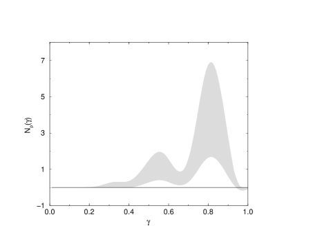
Figure 2: Distribution of intrinsic axial ratios, assuming that clusters are prolate. The shaded region represent the 90% confidence band found by bootstrap resampling of the Mohr et al. (1995) cluster sample.

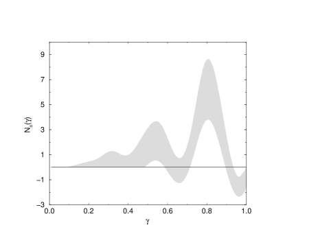
Figure 3: Distribution of intrinsic axial ratios, assuming that clusters are oblate (same as Fig. 2).

In order to obtain constraints on the intrinsic cluster shapes, we use the Mohr et al. (1995) cluster sample. Here, the authors studied 65 nearby clusters and presented apparent axial ratios of these clusters using X-ray isophotal data. This is the largest such study available in the literature, while other studies, involving a less number of clusters, essentially contains more or less the same clusters as the Mohr et al. (1995) sample. Another advantage of the Mohr et al. (1995) cluster sample is that it is X-ray flux limited and clusters were not selected based on the X-ray surface brightness. The original sample in Mohr et al. (1995) was defined by Edge et al. (1990) based on observations by HEAO-1 and Ariel-V surveys combined with Einstein Observatory imaging observations. Such a flux-limited complete, or near-complete, sample, instead of a surface brightness selected sample, has the advantage that clusters are not likely to be biased in their selection. Such selection effects, say due to elongated nature by enhancing the surface brightness, would be problemtic both for the current study on the intrinsic shapes of clusters as well cosmological studies using clusters based on the X-ray luminosity and temperature function. For the purpose of this paper, we assume that clusters in the Mohr et al. (1995) sample has been selected in an unbiased manner when their intrinsic shapes are considered (see, also, Edge et al. 1990).

We use tabulated axial ratio measurements in Table 3 of Mohr et al. (1995), which contains measurements for 58 clusters, to obtain a nonparametric estimates for the underlying distribution. These were then inverted to obtain intrinsic axial ratio distributions, assuming prolate and oblate shapes for clusters. In Figs. 2 & 3, we show our results; the shaded region represent the 90% confidence limits from bootstrap resampling technique. If we assume that all clusters are prolate, the observed distribution is consistent with such an assumption; except when $\gamma\sim 1$, the distribution is always positive. However, if we assume that all clusters are oblate, then the resulting intrinsic distribution is inconsistent with such an assumption at the $\sim$ 98% confidence. Returning to previous works, we find that such a conclusion is consistent with constraints on intrinsic cluster shapes using optical data. In Ryden (1996), for various optically selected samples, randomly oriented oblate hypothesis was rejected at a higher confidence level than the randomly oriented prolate hypothesis. However, we note an alternative possibility that clusters are in fact triaxial ellipsoids. Another possibility is that our assumption that clusters are randomly oriented ellipsoids may be incorrect; clusters can still be oblate ellipsoids, however, they should be oriented in preferred directions than random directions. Since we do not have additional information on such scenario, we may be left with the possibility that clusters are either randomly oriented prolate or randomly oriented triaxial ellipsoids.

2.3 Clusters as Triaxial Ellipsoids

In order to test the possibility that galaxy clusters are triaxial ellipsoids viewed from random angles, we now consider random projections of such objects. It has been shown in Stark (1977; also, Binney 1985) that triaxial ellipsoids project into ellipses when viewed at random angles. Assuming a viewing angle of $(\theta,\phi)$, in a standard polar coordinate system with $z$-axis acting as the pole, the axial ratio of such an ellipse can be written as (Binney 1985; Ryden 1992):

$$q(\beta,\gamma,\theta,\phi)=\left[\frac{A+C-\sqrt{(A-C)^{2}+B}}{A+C+\sqrt{(A-C)^{2}+B}}\right]^{1/2}$$ (11)

where,

$$A= \left(\cos^{2}\phi+\beta^{2}\sin^{2}\phi\right)cos^{2}\theta+\gamma^{2}\sin^{2}\theta,$$

$$B= 4\cos^{2}\theta\sin^{2}\phi\cos^{2}\phi\left(1-\beta^{2}\right)^{2}$$ (12)

$$C= \sin^{2}\phi+\beta^{2}\cos^{2}\phi$$

and $\beta$ and $\gamma$ are the intrinsic axis ratios of the ellipsoid. Following Ryden (1992), where a similar calculation was applied to elliptical galaxies to address their intrinsic shape distribution, we test the possibility that clusters are intrinsically triaxial ellipsoids with axis ratios of ellipsoids distributed according to a Gaussian distribution:

$$f(\beta,\gamma)\propto\exp\left[-\frac{(\beta-\beta_{0})^{2}+(\gamma-\gamma_{0})^{2}}{2\sigma_{0}^{2}}\right],$$ (14)

and the constraint $1\geq\beta\geq\gamma\geq 0$. Here, $\beta_{0}$, $\gamma_{0}$ and $\sigma_{0}$ describe the intrinsic Gaussian distribution and whose parameters can be constrained by a comparison of the observed axial ratios given by Eq. 11. For a set of $\beta_{0}$, $\gamma_{0}$ and $\sigma_{0}$ values, we randomly generate $(\beta,\gamma)$ values that follow the above Gaussian distribution and the associated constraint. We them view each pair of $(\beta,\gamma)$ values with randomly chosen set of viewing angles $(\theta,\phi)$. Following this procedure, we randomly generate $\sim$ 10⁵ $q$ values for which we apply the non-parametric kernel estimator to obtain the underlying distribution. Using $\chi^{2}$ statistic, we compare this underlying distribution to the observed distribution and its error from the Mohr et al. (1995) dataset. Finally, we repeat this procedure for different values of the basic parameters that define the Gaussian distribution.

In Fig 4, we show constraints obtained on the intrinsic shape parameter distribution by comparing to present observations. Here, we show the 99%, 95.4% and 99.99% confidences on $\beta_{0}$ and $\gamma_{0}$ for several values of $\sigma_{0}$. As shown, the observed distribution of axial ratios are consistent when $\beta_{0}$ is at the high end, while $\gamma_{0}$ varies from low values to high values as $\sigma_{0}$ is increased. For low $\sigma_{0}$ values, the observations are more consistent with the possibility that clusters are oblate ($\beta_{0}=1$) rather than prolate ($\beta_{0}=\gamma_{0}$). However, as $\sigma_{0}$ is increased the observed distribution becomes more consistent with the possibility that clusters are intrinsically prolate. Still, we note that there is a large range of possibilities where the observations are consistent with values for $\beta_{0}$ and $\gamma_{0}$ which are neither consistent with the prolate nor the oblate hypothesis. For the parameter space considered here, the best fit model has same $\beta_{0}$ and $\gamma_{0}$ values of 0.92 and $\sigma_{0}=0.21$. The reduced $\chi^{2}$ value of this model and data is 1.1. In general, when $\sigma_{0}>0.1$, statistically acceptable fits are found when $\beta_{0}$ is close to $\gamma_{0}$, suggesting that current cluster data are more consistent with an intrinsically prolate distribution.

Figure 4: Confidence limits on $\beta_{0}$, $\gamma_{0}$ and $\sigma_{0}$ parameter space. Shown here are the $\beta_{0}$ and $\gamma_{0}$ confidences for three values of $\sigma_{0}$ (0.05, 0.15 & 0.25). The contours are at 95.4%, 99% and 99.99% respectively.

3 Discussion & Summary

Using the Mohr et al. (1995) cluster sample, we rule out that clusters are intrinsically axisymmetrical oblate ellipsoids at the 98% confidence level. As the Mohr et al. (1995) cluster sample is a flux limited sample rather than a surface brightness selected sample, we can consider such a sample as a fair representation of clusters in the Universe. Mohr et al. (1995) cluster sample also describes clusters which are now observed both for the SZ effect and the X-ray emission and are used for the determination of the SZ/X-ray Hubble constant. Thus, conclusions based on the Mohr et al. (1995) sample should be valid for what one can expect from current attempts to determine cosmological parameters using SZ and X-ray data of galaxy clusters. We have assumed that cluster X-ray isophotes represent the true shape of galaxy clusters. It may be likely that cluster X-ray isophotes are flattened compared to the intrinsic cluster shapes, and by ignoring this possibility, we may have introduced a systematic bias in this study. However, we note that such bias, if exists, is likely to be small and that compared to other cluster data available to conduct a study on intrinsic cluster shapes, X-ray isophotal axial ratios allow a strong possibility to obtain reliable conclusions on cluster shapes. Also, we note that any correction to the measured Hubble constant due to asphericity is likely to be based on the shape of X-ray isophotes, which is also expected to be similar to SZ isophotes as both essentially measure the same distribution. Therefore, the use of X-ray isophotes to constrain intrinsic shape distribution should be accurate and valid, when considering the cosmological applications.

Our study shows that clusters are more likely to be prolate rather than oblate ellipsoids, however, we cannot rule out the possibility that clusters are intrinsically triaxial. Considering our previous discussions in Cooray (1998) related to cluster projection effects on the SZ/X-ray Hubble constant, intrinsic prolate distributions allow a less biased determination of the Hubble constant, while an intrinsic oblate distribution results in a mean value for the Hubble constant which can be biased as large as $\sim$ 10% from the true value. In Cooray (1998), we only considered the projection effect arising from the unknown inclination angle of galaxy clusters by averaging over a uniform distribution in inclination angles, while only considering a mean value for the axial ratio of clusters from Mohr et al. (1995). Given that we have now determined the intrinsic distribution of axial ratios, we can now extend our calculations presented in Cooray (1998) to also consider intrinsic axial ratio distribution. Here, we assume that SZ and X-ray shape parameters coincide, however, this is only true if clusters are triaxial ellipsoids. If the true shape of clusters were to be more complicated, then a detailed analysis would be necessary to obtain the individual shape parameters associated with SZ and X-ray data and to determine the Hubble constant.

Assuming a simple scenario in which clusters are triaxial ellipsoids, for a cluster sample of 25 clusters randomly drawn from the intrinsic prolate and oblate distributions, we find that the oblate assumption and its distribution results in a biased measurement of the Hubble constant by $\sim$ 8%, while for a prolate distribution, the resulting mean value for the Hubble constant is unbiased, or within $\sim$ 3%. For both prolate and oblate distributions, the width of the resulting distribution of Hubble constant values agree with each other. These estimates both over and underestimates such that true value is within the range. These calculations and ones presented elsewhere (e.g., Sulkanen 1999) suggest that the measurement of the Hubble constant based on galaxy clusters is not fundamentally biased by cluster projection effects and the shape distribution. Therefore, it is likely that a reliable measurement of the Hubble constant will soon be possible with galaxy clusters using SZ and X-ray data, however, such a calculation would still require that we improve our knowledge on cluster physical properties such as isothermality and gas clumping.

References

- [Birkinshaw 1998] Birkinshaw, M. 1998, Physics Reports (in press).
- [Binney 1985] Binney, J. 1985, MNRAS, 212, 767.
- [Binney & Tremaine 1991] Binney, J., Tremaine, S. 1991, Galactic Dynamics (Princeton: Princeton University Press).
- [Branch 1998] Branch, D. 1998, ARA&A, in press (astro-ph/9801065).
- [Cavaliere et al. 1977] Cavaliere, A., Danse, L., De Zotti, 1977, ApJ, 217, 6.
- [Cooray 1998] Cooray, A. R. 1998, A&A, 339. 623.
- [Gunn 1978] Gunn, J. E., 1978, in Observational Cosmology: Advanced Course, 8th, Sass-Fee, Geneva Observatory (Switzerland), pp. 3-124.
- [Hughes & Birkinshaw 1998] Hughes, J. P., Birkinshaw, M. 1998, ApJ, 501, 1.
- [Inagaki et al. 1995] Inagaki, Y., Suginohara, T., Suto, Y. , PASJ, 47, 411.
- [Lucy 1974] Lucy, L. B. 1974, AJ, 79, 745.
- [Merritt & Tremblay 1994] Merritt, D., Tremblay, B. 1994, AJ, 108, 514.
- [Mohr et al. 1995] Mohr, J. J. et al. 1995, ApJ, 447, 8.
- [Perlmutter et al. 1998] Perlmutter, S., Aldering, G., Valle, M. D., et al. 1998, Nature, 391, 51.
- [Riess et al. 1998] Riess, A. G., Filippenko, A. V., Challis, P., et al. 1998, AJ, 116, 1009.
- [Roettiger et al. 1997] Roettiger, K., Stone, J. M., Mushotzky, R. F. 1997, ApJ, 482, 588.
- [Ryden 1992] Ryden, B. S., 1992, ApJ, 396, 445.
- [Ryden 1996] Ryden, B. S., 1996, ApJ, 461, 146.
- [Sulkanen 1999] Sulkanen, M. E., 1999, ApJ, in press (astro-ph/9903379).
- [Sunyaev & Zeldovich 1980] Sunyaev, R. A., & Zel’dovich, Ya. B., 1980, ARA&A, 18, 537.
- [Silk & White 1978] Silk, J., White, S. D. 1978, ApJ, 223, L59.
- [Silverman 1986] Silverman, B. W. 1986, Density Estimation for Statistics and Data Analysis (New York: Chapman & Hall)
- [Stark 1977] Stark, A. A. 1977, ApJ, 213, 368.
- [Vio et al. 1994] Vio, R., Fasano, G., Lazzarin, M., Lessi, O. 1994, A&A, 289, 640.