A 33 GHz interferometer for CMB observations on Tenerife

Abstract

We describe a new high sensitivity experiment for observing cosmic microwave background (CMB) anisotropies. The instrument is a 2-element interferometer operating at 33 GHz with a $\sim$3 GHz bandwidth. It is installed on the high and dry Teide Observatory site on Tenerife where successful beam-switching observations have been made at this frequency. Two realizations of the interferometer have been tested with element separations of $11.9~{}\lambda$ and $16.7~{}\lambda$ . The resulting angular resolution of $\sim 2^{\circ}$ was chosen to explore the amplitude of CMB structure on the large angular scale side of the Doppler (acoustic) peak. It is found that observations are unaffected by water vapour for more than 70 per cent of the time when the sensitivity is limited by the receiver noise alone. Observations over several months are expected to give an rms noise level of $\sim 10-20~{}\mu$K covering $\sim$100 resolution elements. Preliminary results show stable operation of the interferometer with the detection of discrete radio sources as well as the Galactic plane at Dec = +41°  and $-$29°.

1 Introduction

The detection of angular structure in the cosmic microwave background (CMB) gives a wealth of cosmological data. Observations in the angular range 100°  to 0$\aas@@fstack{\circ}$1 or less can constrain such cosmological parameters as $\Omega_{0}$, $\Omega_{B}$, $H_{0}$ and the spatial spectral index $n$. On the larger angular scales (say $>$5°) the tensor component contribution can be quantified relative to the scalar Sachs–Wolfe contribution. Advances in this field require a good coverage of the angular spectrum at high sensitivity.

Our experiments on the 2400 m high Teide Observatory site on Tenerife have been of the beam-switching type and covered the angular range $\sim$4°  to 16°  by switching a 5°  beam through angles of $\pm$8°  [Davies et al. 1996]. Through the use of scaled experiments at 10, 15 and 33 GHz, we can separate the Galactic and CMB components [Hancock et al. 1994, 1997]. These experiments have provided the first detection of individual hot and cold features which have now been confirmed by an independent observing group [Lineweaver et al. 1995, Gutiérrez et al. 1997].

We describe here a new high sensitivity interferometer system, also located at Teide Observatory, which can investigate structure on 2°  angular scales. The separation of the horn elements can be increased to explore angular scales as small as 1°. With longer baselines the effective “filling factor” would be too small for sensitive measurements. The 1 to 2°  range of angles is on the large scale side of the first of the Doppler (acoustic) peaks produced by photon and matter sources which lead to a maximum amplitude at around the horizon scale at last scattering [White, Scott & Silk 1994]. The interferometer will be used to measure the slope of the CMB spatial spectrum over this range. A frequency of 33 GHz was chosen, a frequency at which we have already shown that the Galactic component $\Delta T_{\rm rms}<5\;\mu$K [Hancock et al. 1997] at $5\degr-15\degr~{}$ angular resolution. On angular scales of $1\degr-2\degr$ this will be significantly less [Lasenby 1996, Veeraraghavan & Davies 1997]. The corresponding CMB $\Delta T_{\rm rms}$ is expected to be $50-100~{}\mu$K. Furthermore, a particular advantage of an interferometer is its much stronger rejection of atmospheric fluctuations compared with a beam-switching system [Webster 1994, Church 1995]. Meteorolgical features subtending angles larger than the interferometer lobe size do not produce a large correlator output signal. However, even smaller features can be supressed if there is some east–west motion of the “cloudlets” through the beam. During an integration the correlator output signal rotates in phase, effecting a cancelation. The cloudlets appear stretched in the direction of motion, and with even a small east–west component this tends to quench the interferometer response.

In this paper Section 2 describes the design concepts and realization of the interferometer while in Section 3 we assess the performance of the instrument. Section 4 contains information on the ability of the interferometer to reject atmospheric effects, and Section 5 describes astronomical commissioning observations with two configurations of the interferometer. The future astronomical programme is outlined in Section 6.

2 Description of the interferometer system

The interferometer system was built and tested at Jodrell Bank and then moved to Teide Observatory, Izaña, for observations. This observing site has low levels of precipitable water vapour (pwv $<$ 2 mm) for much of the year and permits the collection of high quality data from the 33 GHz beam-switching radiometer for $\sim$20 per cent of the time. It was anticipated that an interferometer at this frequency would be usable for a much higher fraction of the time; our experience confirms this and is quantified in Section 4.

High sensitivity to CMB anisotropy can be achieved by using cryogenically cooled low noise receiver systems operating with large ($\sim$10 per cent) bandwidths. The required sensitivity of $\sim$10 $\mu$K per resolution element is obtained by repeated observations of the chosen area of sky. The design of the interferometer described below owes much to the experience accumulated with the 5 GHz wide bandwidth interferometer operated at Jodrell Bank [Melhuish et al. 1997].

2.1 Concept of the CMB interferometer

The interferometer consists of two horn apertures fixed in an east–west line. Earth rotation then sweeps the interferometer fringe pattern across the sky giving 24^h  coverage in right ascension (RA) each day. The declination of observation is set by tilting the interferometer assembly in the meridian plane to the appropriate elevation. The physical arrangement is shown in Fig. 1. The aim is to make a high sensitivity map of the band of sky, centred on Dec = +41°, that has been explored on somewhat larger angular scales at 5, 10, 15 and 33 GHz [Melhuish et al. 1997, Gutiérrez et al. 1995, Gutiérrez et al. 1997, Hancock et al. 1997].

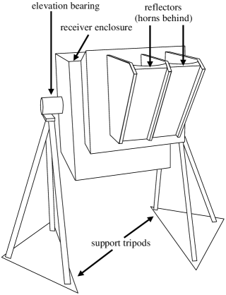
Figure 1: A three dimensional representation of the interferometer in the $16.7~{}\lambda$ configuration. A weather–sealed box contains the cooled receivers and the correlator, with the horn-reflector antenna system projecting from the front face. The assembly may be rotated in the elevation direction upon its support tripods.

The operating frequency was chosen to be 33 GHz where our previous experience with beam-switching radiometers on $5\degr-15\degr$ angular scales indicated a level of Galactic contamination less than 10 per cent of the intrinsic CMB fluctuation amplitude. Since the interferometer is sensitive to structures with smaller angular scales, it is expected that any Galactic contribution will be less still, because of the downwards slope of the Galactic spatial power spectrum. On the 2° angular scale of this interferometer both the synchrotron [Lasenby 1996] and the free–free [Veeraraghavan & Davies 1997] Galactic components will be a factor of 2 – 4 less than found in our Tenerife beam-switching observations. Moreover, at this frequency the atmospheric contamination of the signals observed with the interferometer will be substantially lower than that experienced with the 33 GHz beam-switching radiometer at Teide Observatory. The system was designed to have a 3 GHz (10 per cent) bandwidth which can be readily realized using analogue technology for the correlator.

The design aim was to achieve a resolution of $2\degr\times 2\degr$. To obtain the highest brightness temperature sensitivity, the receiving horns were placed adjacent to one another leaving only a small $\sim$10 mm gap. By choosing a primary beam of $5\degr\times 2\degr$ elongated in the EW direction, a synthesized beam measuring approximately $2\degr\times 2\degr$ can be produced by the interferometer response.

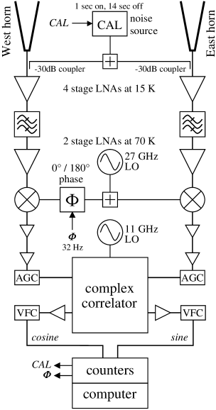
Figure 2: A schematic diagram of the interferometer. Shown from the top, down, are: the antennas and calibration system, the low noise receivers, the down–conversion system, the automatic gain control, the correlator and finally the logging system.

Although the receiving antennas have low sidelobes screening is placed around the interferometer to reduce further the likelihood of coherent signals entering the feed horns from stray ground radiation. The screens also minimize the level of interfering RF signals. Fig. 2 is a schematic diagram of the interferometer. A description of the various components of the system is given in the following sub-sections.

2.2 The antenna system

Two realizations of our antenna concept were constructed and used for astronomical observations. The first, a pyramidal horn system, had an element separation of $11.9~{}\lambda$  while the second realization, a horn-plus-reflector system, had a $16.7~{}\lambda$   element separation.

(a)The pyramidal horn design — $11.9~{}\lambda$ spacing. The E–W beam response is provided by a 100 mm H-plane aperture while the narrower N–S beam response is achieved by using a 410 mm aperture across which the phase variations are corrected by a dielectric lens inside the aperture. The depth of the horn is 480 mm. The polar diagram of each horn is $5\degr\times 2\degr$ in the ${\rm E}\times{\rm H}$ (${\rm EW}\times{\rm NS}$) directions. The spacing between horn centres is $11.9~{}\lambda$  (110 mm) in the EW direction to give an interferometer fringe period of 4$\aas@@fstack{\circ}$7. The high side-lobe level of this design can be seen in Fig. 3. Astronomical measurements to be described below indicate that the desired FWHP (full width at half power) was achieved although the aperture efficiency was only $\sim$0.3.

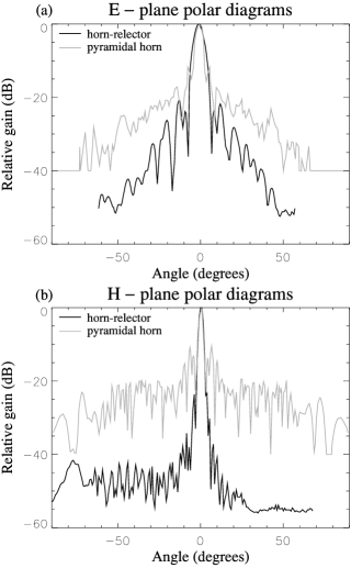
Figure 3: The polar diagrams for the original pyramidal horns, and the horn-reflector antennas. (a) shows the E-plane (horizontal) cut and (b) shows the H-plane (vertical) cut.

Figure 4: The window functions for three antenna spacings. The spectral power density sensitivity, $W_{l}$, is plotted as a function of spherical harmonic, $l$. The $11.9~{}\lambda$ and $16.7~{}\lambda$ plots are for the pyramidal horn and horn–reflector antennas respectively. The $33.4~{}\lambda$ plot shows the response for the next spacing to be used.

(b)The combined horn-reflector design — $16.7~{}\lambda$ spacing. The required low side-lobe and high aperture efficiency on the desired angular scale can best be realized by illuminating a parabolic section reflector with a corrugated horn. A detailed description will be given by Dicker, Withington & Gassan (in preparation). The physical aperture of each feed is 140 mm (E–W) $\times$ 400 mm (N–S) again with the E-plane N–S. The FWHP is $5\degr\times 2\aas@@fstack{\circ}5$ (${\rm EW}\times{\rm NS}$) and the antennas are separated by $16.7~{}\lambda$  (152 mm) centre-to-centre. Fig. 3 shows the E and H-plane polar diagrams. A low side-lobe level is achieved which is consistent with a calculation that 91 per cent of the power is within 10 dB of the beam centre, compared with 93 per cent for a Gaussian beam profile.

The window functions of the different antenna configurations are illustrated in Fig. 4. This shows the sensitivity of the telescope, $W_{l}$, to power at different values of the spherical harmonic number, $l$, for $11.9~{}\lambda$ and $16.7~{}\lambda$ spacings. The response for a spacing of $33.4~{}\lambda$ is also shown, where we will be collecting data in the future. Fig. 4 shows that increasing the antenna separation reduces the sensitivity of the telescope, but it should be remembered that this is largely offset by the reduced weather effects at larger separations.

2.3 The RF and IF stages

Radio frequency (RF) signals are received by the two horns with the E-vector in the vertical plane. They are then taken by waveguide into the cryostat. This is cooled by a Gifford-McMahon closed-cycle refrigeration system, using compressed gaseous helium. The RF voltages in each channel of the interferometer are amplified in a 4-stage low noise amplifier (LNA) with a gain of 25 dB, cooled to a physical temperature of $\sim 15$ K. A second 2-stage amplifier, cooled to 70 K, supplies a further 12 db of gain. When cooled the first amplifiers have noise temperatures between 60 and 80 K, while the second amplifiers have somewhat higher noise-temperatures but only contribute $\sim 1$K to the overall noise temperature. These amplifiers are constructed at Jodrell Bank from Fujitsu FHR10X devices. The operating bandwidth is defined by a 5-pole waveguide filter between the two LNAs in each RF channel. The measured RF band is 2.6 GHz wide at 3 dB and is centred at 32.5 GHz.

An item crucial to achieving a robust and stable operation of the interferometer is the calibration noise signal (CAL) which is coupled to each input waveguide. The noise source is a noise diode with an excess noise ratio of $\sim$25 dB. Its output is fed through a variable attenuator, then a 3 dB splitter into a -30 dB cross-guide coupler on each input waveguide to give a calibration signal of $\sim$10 K. This CAL signal has two functions; firstly it provides a monitor of the gain of the system and secondly it gives a phase reference for the interferometer. This enables successive days of data to be added in the correct amplitude and phase. CAL is switched on for 1 sec every 15 sec.

The RF signals from each amplifier chain are fed to a DC-biased mixer where they are mixed with signals from a common Gunn diode local oscillator source (LO), operating at 27 GHz. As shown in Fig. 2, the LO signal for the West channel has a (0°, 180°) phase switch which modulates the sign of the correlated output at a switch frequency of 32 Hz driven from the control computer.

The IF signals from each mixer leave the cryostat and are amplified in broad-band amplifiers located on a temperature stabilised plate. Each IF channel has four gain stages, with a total gain of $\sim$90 dB. The West IF line contains a trombone line which can be adjusted to make the path length the same in the two arms of the interferometer. This sets the interferometer on the “white light fringe”. An automatic gain control (AGC) system can attenuate the IF power levels by up to 20 dB to achieve constant levels at the correlator inputs.

2.4 The Correlator

The correlator has been designed for the wide bandwidth of 3 GHz used in the present interferometer. Correlators conventionally used in long baseline interferometers are of the digital type so as to readily implement the continuous path length compensation required. The present short baseline drift-scan interferometer does not require this and so can employ the less technically demanding analogue-analogue correlation scheme.

The block-diagram of the complex correlator with cosine and sine outputs is illustrated in Fig. 5. Conceptually the design follows that of the 5 GHz short baseline interferometer which has operated successfully at Jodrell Bank [Melhuish et al. 1997]. However the new design is for a bandwidth of 3 GHz rather than 0.4 GHz and the realization takes account of this much larger bandwidth requirement. The orthogonal outputs are formed using a second stage of mixing with a second LO at 11 GHz. This LO signal is fed to the West IF mixers M1 and M2 via the in-phase and quadrature (0°  and 90°) splitter S3, so that two West second IF signals are produced, one 90° behind the other. The East IF is mixed with an LO signal in M3 to give the East second IF. Finally, the two West second IF signals are each mixed with the East second IF signal (at the same phase) in mixers M4 and M5 which act as multipliers to produce cosine and sine outputs.

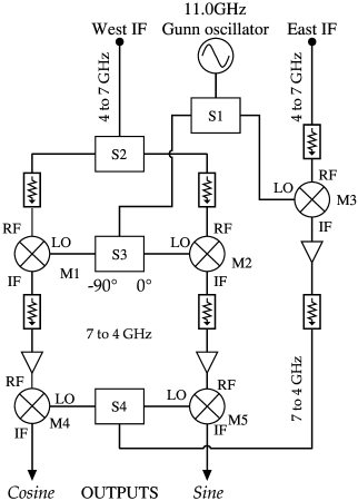
Figure 5: The correlator. Splitters are labelled S1 to S4 and the mixers are M1 to M5. S3 is a hybrid splitter, producing LO signals in phase-quadrature. This results, finally, in quadrature output signals from M4 and M5.

The phase difference between the cosine and sine output channels was kept close to 90°  by careful control of electrical path lengths. This difference was found to be 85°  from measurements of astronomical signals. The analysis software orthogonalizes the output channels. The efficiency of the correlator was measured to be 0.78$\pm$0.08.

The outputs from the cosine and sine channels are applied to synchronous voltage-to-frequency converters (SVFC) and the output pulses are sent to the control / logging computer.

2.5 Control and data acquisition system

The computer operating the interferometer also performs the function of data acquisition and storage. It keeps an accurate time record for registering the data by reference to a “Stratum 2” time server. A 32 Hz square-wave is generated to supply the control voltage for the phase switch on the channel 1 side of the first LO. The same square wave drives the software phase sensitive detectors (PSD) which produce the cosine and sine data streams, de-modulating the 32 Hz square waves produced by phase-switching. An integration cycle generates a 30 sec sequence of data. During this cycle the CAL noise diode is switched on twice for 1 sec each time.

The cosine and sine 16 msec data streams, and other critical parameters, are used to produce mean and rms values for each 30 sec cycle. The rms values provide a monitor of the performance of the system on this time scale. The following quantities are recorded:

1. Time

2. PSD level: cosine and sine

3. CAL level: cosine and sine

4. rms on PSD: cosine and sine

5. rms on CAL: cosine and sine

6. First IF power: west and east channels

7. Temperature monitors within instrument enclosure.

The local meteorology in the form of temperature and humidity from a Stephenson screen is recorded by the adjacent beam-switching experiments.

Fig. 6 is a plot of some of the data streams from 24 May 1997. Shown are the PSD outputs (cosine and sine), rms of the PSD outputs, and the IF power in the east receiver. Note that the Sun is visible at UT = 13^h00^m in the side-lobes at a level $\sim$-46 dB relative to the beam centre. The Cygnus A and Cygnus X transit is seen at RA = 20^h00^m - 21^h00^m with the instrument set at Dec = +41$\aas@@fstack{\circ}$0. The rms in the 30 sec integrations is 0.48 and 0.45 mK in the cosine and sine channels respectively.

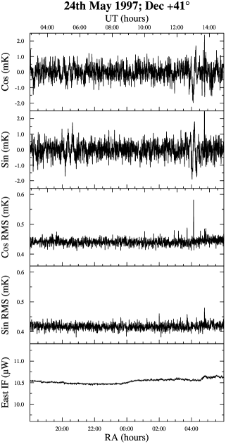
Figure 6: Data from 24 May 1997. Shown are the cosine and sine data channels, their errors, and the IF power in the east receiver. At 4^h00 RA fringes due to the Sun in the side-lobes can be seen. At around 20^h00 RA, structure from the Cygnus region is visible. At all times the data are limited only by receiver noise.

3 Instrumental performance

The interferometer was assembled at NRAL, Jodrell Bank, and tested as far as possible before being shipped to Tenerife for final installation in a 2.5 m–high aluminium-screened enclosure at Teide Observatory. The enclosure extends $\sim$ 1 m above the level of the interferometer horns. This dry site gave the conditions appropriate for astronomical tests and calibration prior to the definitive astronomical programme of long-term repeated daily observations to achieve the deep integrations required to detect CMB structures.

3.1 The interferometer response

We determined the beam response of the interferometer by using transits of the Sun and the Moon. For angles closer than $\sim$10°  to the main beam the response can be modelled in terms of a two-dimensional Gaussian modulated by a sinusoidal function in RA:

$$\exp\left[\frac{\Delta_{1}^{2}}{2\sigma_{1}^{2}}\right]\exp\left[\frac{\Delta_{2}^{2}}{2\sigma_{2}^{2}}\right]\times\left\{\begin{array}[]{ll}\cos\omega\Delta_{1}&\mbox{\rm cosine channel}\\ \sin(\omega\Delta_{2}+\phi)&\mbox{\rm sine channel}\end{array}\right.$$

where $\Delta_{1}$ and $\Delta_{2}$ are the distances in RA and Dec between the centre of the beam and the source; $\sigma_{1}$ and $\sigma_{2}$ represent the width of the beam in RA and Dec respectively; $\omega=2\pi/T$ where $T$ is the separation (in the RA direction) of the fringes on the sky; and $\phi$ is the offset from quadrature of the two channels (Section 2.4).

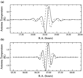
Figure 7: Moon crossings from the two interferometer configurations. (a) is from 1 July 1996 when the interferometer has an antenna separation of $11.9~{}\lambda$  while (b) is from 13 April 1997 with a separation of $16.7~{}\lambda$ . The moon semi–diameters on these dates where 16′39$\aas@@fstack{\prime\prime}$4 and 15′5$\aas@@fstack{\prime\prime}$8 respectively. The solid line represents the sine channel while the dashed line is the cosine channel.

Fig. 7(a) shows the cosine and sine channels with the interferometer in the $11.9~{}\lambda$ configuration. The fringe separation, corrected for the movement of the Moon, was measured to be 4$\aas@@fstack{\circ}$8, and is as expected for the horn separation at 32.5 GHz ($\lambda=9.2$ mm). Although a Gaussian gives a good fit to the main beam response, the side-lobes become increasingly dominant at levels more than 20 dB below the beam peak. As a consequence astronomical data were only used at times when the Sun was below the elevation of the aluminium screen which in practice meant night time only for this configuration.

Fig. 7(b) shows the Moon transit observed with the $16.7~{}\lambda$ system. The fringe period was measured to be 3$\aas@@fstack{\circ}$5 as expected for this spacing. The low side-lobe response shown in Fig. 3 was confirmed by transits of the Sun in the side-lobes, during drift scans at Dec = +41°. With these low side-lobes data can be collected to within $\pm 1$ hour of local noon.

3.2 The receiver performance

Hot and cold load measurements gave a system noise estimate for both receivers of 120 K. Laboratory tests indicated that 80 K of this total came from the LNAs. The atmosphere on a typical dry day contributes 10K, mainly due to O₂. We associate the additional 30 K with the antenna, the input waveguide system, the CAL cross-guide coupler and the input isolator.

The directly measured bandwidth of the receiver system was 2.6 GHz at the $-3$ dB (half power) points and $\sim$3.5 GHz at -10 dB. These values were confirmed by measurements of the width of the white light fringe from the CAL signal by varying the length of the trombone line.

The rms noise recorded continuously in our CMB experiments, from the data streams sampled at 16 msec intervals, is an effective monitor of system performance. The operating noise level is typically 2.2 ${\rm mK.s}^{-1/2}$. This is close to the theoretical value expected for a correlator efficiency of 0.8 and a bandwidth of 2.6 GHz. The values of system performance for the earlier pyramidal horn interferometer system were slightly worse than described above.

3.3 Calibration

The day-to-day temperature calibration of the interferometer is made through the noise diode signal injected into the input waveguides. This gives a continuous monitor of the temperature in the correlator cosine and sine outputs. In order to convert the output data to a temperature scale we use frequent observations of the Moon which is taken to be a circular disc of brightness temperature $T_{b}$ at 33 GHz:

$$T_{b}=214-36\cos(\phi-\epsilon)\>\>\>{\rm K}$$

where $\phi$ is the phase of the moon (measured from full moon) and $\epsilon=41\degr$ is the phase offset resulting from the finite thermal conductivity of the Moon [Hagfors 1970]. As a consequence of the dilution in the main beam of the interferometer, the temperature actually measured for the moon is comparable in size to the calibration signal, CAL. Hot and cold load measurements on the input of the interferometer give results consistent with the Moon and Sun (T_b = 9000 K) observations. A temperature calibration for CMB measurements using an astronomical object (the Moon) is robust since it employs the entire instrument, removing the effects of any receiver non-linearities or sources of de-correlation in the interferometer, and taking into account uncertainties in the efficiency of the beam. Such a scale can be directly linked to other CMB structure measurements which also observe the Moon.

A further astronomical check on the temperature can be made by observing point sources of known flux density. The effective area of the horn–reflector antennas gives a conversion factor of 6.46 $\mu$K/Jy. Measurements of the Crab Nebula (Tau A) agree with the calibration obtained using the Moon.

4 Atmospheric effects at 33 GHz

The effect of atmospheric water vapour on the response of the 33 GHz interferometer has been quantified during the commissioning observations. A preliminary assessment has already been given by Davies et al. (1996) of the atmospheric effects on the CMB observations with the 10, 15 and 33 GHz beam-switching instruments, also located at an altitude of 2400 m at Teide Observatory. As expected from a theoretical analysis [Webster 1994, Church 1995], the atmospheric fluctuations on the smaller angular scales sampled by the interferometer are significantly less than those observed with the beam-switching experiments. We now quantify these atmospheric effects observed at 33 GHz.

4.1 The correlator and total power outputs compared

The data streams from the 33 GHz interferometer include the total radio frequency power levels, measured at each first IF. The total power record gives the total intensity from the sky (including water vapour emission) in the main beam of the interferometer. The cosine and sine outputs give a measure of the correlated signal in the interferometer lobes. A comparison can be made of the total power and interferometer outputs over a period of high water vapour content for each configuration of the interferometer.

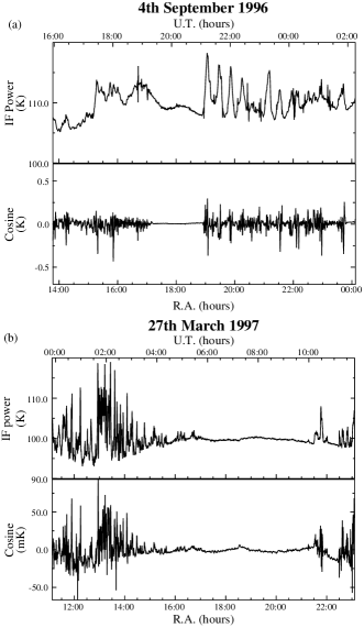
Figure 8: Plots showing the rejection of atmospheric water vapour effects by the interferometer, on days of bad weather. The upper part of each plot shows the total power fluctuations observed in the primary beam; the lower part of each plot shows the fluctuations on the interferometer cosine output. (a) $11.9~{}\lambda$ baseline observed on 4 September 1996 (b) $16.7~{}\lambda$ baseline observed on 27 March 1997. The $\sim$10 K fluctuation in the total power records are reduced by a factor of $\sim$100 in the short baseline data and $\sim$200 in the longer baseline data.

Fig. 8(a) shows the total power and cosine records for the night of the 4 September 1996 with the interferometer in the $11.9~{}\lambda$ configuration. 10–20 K fluctuations in the total power on time-scales of 30 s are reduced to $\sim$200 mK at the cosine and sine outputs. A short period of receiver noise limited data occurs around 20^h UT. Fig. 8(b) shows a similar data set covering the morning of 27 March 1997 when the interferometer was in the $16.7~{}\lambda$ configuration. The rejection of atmospheric effects is even more pronounced than in Fig. 8(a), with the amplitude of fluctuations in the IF power being reduced by a factor of $\sim$200 in the interferometer data.

A quantitative estimate of the ratio between the interferometer output and the total power can be made by comparing the amplitude of the interferometer output calculated from the cosine and sine channels with the total power channel. This ratio is $\sim$1:100 for the $11.9~{}\lambda$ and $\sim$1:200 for the $16.7~{}\lambda$ baselines. The difference in ratio for the two baselines is in the sense predicted by Webster [Webster 1994]. A more detailed study of the atmospheric effects seen in the interferometer will be published separately by Watson & Davies (in perparation).

4.2 The interferometer compared with beam-switching

A comparison of atmospheric fluctuations in the beam-switching and interferometer experiments at 33 GHz gives information about the angular spectrum of atmospheric structure above the Teide Observatory. The beam-switching experiment measures the difference between the temperatures seen in a 5${}^{\circ}\times$ 5°  beam switched $\pm$8°  while the interferometer forms adjacent positive and negative lobes approximately 2${}^{\circ}\times$ 2°  in size. Hence the angular scales sampled in the two experiments differ by a factor of about 4.

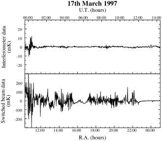
Figure 9: A comparison of atmospheric water vapour fluctuations observed with the 33 GHz interferometer and beam-switching systems on 17 March 1997, a day of bad weather. The interferometer (upper part) was in the $16.7~{}\lambda$ baseline configuration, set to dec = +41°. The switched beam experiment was set to dec = +35°. The interferometer is receiver noise limited for $\sim$50 per cent of the time, and even when it is not the weather effects are 30 – 50 times smaller than in the beam-switching experiment.

The response of the beam-switching and the interferometer systems to a period of strong water vapour activity experienced on 17 March 1997 is illustrated in Fig.9. The activity was associated with cloud; periods of clear sky, with a low level of water vapour, occur before and after the active phase. Peaks in the beam-switching output are several 100 mK while those in the interferometer are a few mK. A quantitative comparison of the amplitude of the beam-switching and interferometer variations due to water vapour gives a ratio of 50:1. These data are for the $16.7~{}\lambda$ baseline. Some small modification of this value may be required to account for the difference in declination setting of the two experiments. Further, the fluctuation amplitude is derived from 82 sec integrations in the beam-switching experiments and $\sim$30 sec integrations in the interferometer. The effect of the latter is to increase the ratio of beam-switching to interferometer fluctuation amplitudes by a few tens of per cent.

Because of the smaller atmospheric effects on the interferometer data, the fraction of useful data is significantly higher than for the 33 GHz beam-switching experiment. This situation is shown quantitatively in Fig.10 which is a cumulative plot of the observed rms noise for the raw data sets of the 33 GHz beam-switching and interferometer experiments. The plots are for night-time data taken during September 1995, a period when the water vapour content begins to rise following the drier summer months. Data for the plots were the mean rms signals, examined in 30^m  and 12^m  RA intervals for the beam-switching and interferometer data respectively; these intervals correspond approximately to the angular scale of maximum sensitivity for sky signals in each experiment. We see that the fraction of data with an rms less than that expected for receiver noise alone is a few per cent for the beam-switching and $\sim$50 per cent for the interferometer. Hence the time for which observing conditions are suitable for interferometry at 33 GHz is many times greater than for beam-switching observations. In a one year period the availability of the interferometer is $\sim 70-80$ per cent, compared with $\sim 20$ per cent for the radiometer. This topic will be examined in more detail in the paper by Watson & Davies (in preparation).

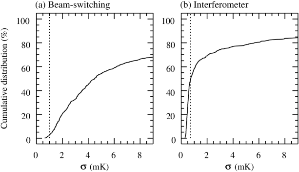
Figure 10: Cumulative noise statistics for the beam-switching radiometer (left) and interferometer (right) for September 1995, during a period of increased water vapour activity. The dotted lines represent the expected rms due to receiver noise alone. In the absense of other sources of noise we should expect the cumulative distribution to reach approximately 65 per cent by this point. The fact that for the radiometer the percentage is much smaller shows that it is severely affected by weather. The interferometer is less affected.

5 Astronomical tests of the interferometer

In this section we describe astronomical tests which demonstrate that the interferometer has the necessary sensitivity and stability to detect CMB fluctuations with $\Delta T_{\rm rms}\>\sim$50 $\mu$K when a realizable amount of data are stacked. Any strong astronomical source can be clearly detected when data from a number of transits are stacked. In the case of the strong sources, Tau A, Cyg A, Cyg X and Cas A, approximately 10 transits are sufficient. The normal observing procedure is to take RA drift scans of 24^h  duration with the interferometer set at a fixed declination. This technique ensures that any correlated pick-up from the ground remains fixed, thereby contributing to the stability of the baselines.

With the $11.9~{}\lambda$ baseline (pyramidal horns) only night-time data could be used, while with the $16.7~{}\lambda$ baseline (horn + reflector design) data could be taken up to within $\pm 1$ hour of the Sun transit.

5.1 Dec = +41°  scans

This declination was chosen for observation because it lies in the centre of the region that we have been using for our deep surveys of CMB fluctuations [Davies et al. 1996, Hancock et al. 1997] and for the present purposes it contains the extragalactic radio source Cyg A (RA = 19^h59^m, Dec = 40°44′, J2000) and the Galactic HII complex Cyg X [Pike & Drake 1964] which covers an area bounded by RA = 20${\rm{}^{h}15^{m}}$ to 20${\rm{}^{h}45^{m}}$ and Dec = 38$\aas@@fstack{\circ}$5  to 44$\aas@@fstack{\circ}$0. Fig. 11 shows the cosine and sine plots of the Dec = +41°  stacks taken with the $11.9~{}\lambda$ and $16.7~{}\lambda$ baseline configurations. The complex structure in Cyg X gives different responses in the two interferometer configurations as expected. The longer baseline just separates Cyg A (flux density S = 35$\pm$7 Jy) from Cyg X at the expected temperature of 230 $\mu$K for the sensitivity of T = 6.46 $\mu$K for 1 Jy. Away from Cyg A and X the data are noise-limited with $\Delta T_{\rm rms}\sim$50 $\mu$K in 2 min integrations stacked over approximately 10 days. This is the value expected for the measured system noise and bandwidth with a correlator efficiency of $\sim 0.8$. If the performance improves as expected, on further stacking and data processing an rms of 6 $\mu$K per beam would result from the addition of 100 scans. The data must then be corrected for the dilution of the sky signals in the interferometer lobes compared with the primary beam envelope. The size of this correction depends strongly on scale size, and the model assumed for the CMB power spectrum and will be discussed in later papers.

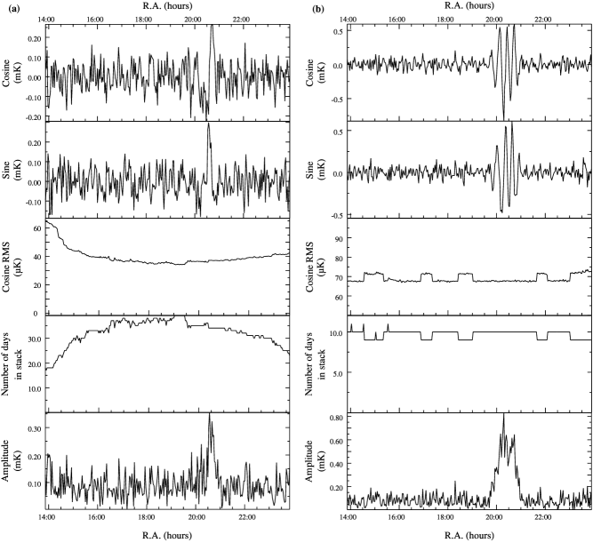
Figure 11: Stacks of data taken at Dec = +41°; (a) Data taken with the $11.9~{}\lambda$ antenna spacing; (b) Data taken with the $16.7~{}\lambda$ antenna spacing. The data were taken over October/November 1995 and April 1997 respectively. Only the rms values for the cosine channel are shown as they are very similar to the sine rms values. Each point represents an integration over 2 minutes of RA.

5.2 Observations of Cas A and Sgr A

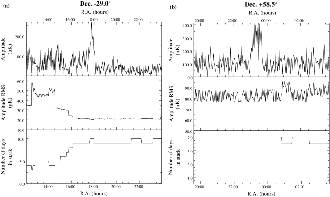
Figure 12: Sgr A (left) and Cas A (right) as seen by the interferometer with a $11.9~{}\lambda$ spacing. For each source, the amplitude $(\sin^{2}+\cos^{2})^{1/2}$, the rms error of this, and the number of days of observations at each RA, are shown. All these observations were taken over September – November, 1996

Fig. 12 shows the amplitude and rms noise plots for Cas A and Sgr A. The interferometer was set at the declination of Cas A (RA = 23^h23^m, Dec = 58°49′, J2000) and 7 scans from September 1996 were added to give the plot in Fig. 12(b). The dimensions of Cas A ($6\arcmin\times 6\arcmin$) make it unresolved by the interferometer beam. The flux density expected at 33 GHz, taking account of its secular decrease in intensity [Baars et al. 1977] is 162$\pm$19 Jy at the present epoch so the expected antenna temperature is $\sim$400 $\mu$K for the pyramidal horn antennas. This is the observed value.

The stack of 10 scans through Sgr A (RA = 17^h46^m Dec = $-29^{\circ}$00′, J2000) is shown in Fig. 12(a). A signal amplitude of 250 $\mu$K is observed. For the pyramidal horn configuration this temperature corresponds to a flux density of $\sim$120 Jy. Little published information is available on the 33 GHz brightness distribution in the Galactic centre region. The central $2\degr\times 2\degr$ contains both synchrotron and free-free emission on a range of angular scales [Mezger & Pauls 1979]. The observed flux in the interferometer lobes is not unreasonable.

Both the Cas A and Sgr A stacks give $\Delta T_{\rm rms}\sim$50 $\mu$K in a 2 min integration for a stack containing $\sim$10 scans. This is consistent with the Dec = +41°  scans and indicates that the performance of the interferometer is not being affected by the weather in any subtle low-level way since these observations were made at various times throughout the year and at various elevation angles (declinations).

6 Conclusions

We have demonstrated the potential of interferometric CMB observations at 33 GHz from the Teide Observatory in Tenerife, at an altitude of 2400 m. This instrument will extend to 2°  the angular range of CMB fluctuations observed in the Tenerife CMB project which at present covers the range 5°  to 15°. We describe the design and performance of this broad-band, short-baseline interferometer and demonstrate its phase stability and sensitivity with observations of Cyg A, Cyg X, Cas A and Sgr A.

The interferometer shows an improvement in atmospheric fluctuation rejection over the 33GHz beam-switching radiometer, which has its peak sensitivity on 8°  scales, by a factor greater than 30. This allows the interferometer to observe for 70 – 80 per cent observing efficiency on the site at 2°  scales and vindicates the choice of Tenerife for interferometry and the Very Small Array [Jones 1998].

The first observations with the 2°  interferometer will be a deep scan at Dec = +41°  to explore the CMB fluctuation field at high Galactic latitudes. This area of the sky has been covered with a deep survey at 10, 15 and 33 GHz which has already shown that the Galactic foreground contribution is smaller ($<$10 per cent) than the CMB fluctuation level at 33 GHz on 8°  scales; the Galactic contribution will be significantly less than this on the smaller, 2°, scale of the interferometer [Davies & Wilkinson 1998].

Based on the observations reported here for the horn-reflector interferometer we estimate that the noise $\Delta T_{\rm rms}$, on the antenna temperature, for a stack of 100 scans will be 20 $\mu$K in a 2 min interval in RA. By combining data from over the $\sim$20 minute interferometer response pattern, this becomes $\sim$6 $\mu$K per beam. On conversion to sky temperature this becomes 20 $\mu$K per beam. We expect to cover at least two such 24^h  RA strips per year and to generate a sky map with $\sim$500 beam areas; this will result in an error of $5-10$ per cent from cosmic sample variance considerations. We believe that the calibration error will be less than 10 per cent. Based on these estimates we expect an accuracy in determining the $\sim 50~{}\mu{\rm K}$ CMB signal on a 2° scale of $\sim 10$ per cent. By changing the antenna spacing it is possible to obtain data covering an angular scale $1\degr-2\degr~{}$ which will enable us to explore the rise to the first Doppler peak.

References

- [Baars et al. 1977] Baars M.W.M., Genzel R., Pauliny-Toth I.I.K., Witzel A., 1977, AA, 61, 99
- [Church 1995] Church S.E., 1995, MNRAS, 272, 551
- [Davies et al. 1996] Davies R.D., et al., 1996, MNRAS, 278, 883
- [Davies & Wilkinson 1998] Davies R.D., Wilkinson A., 1998, in Bouchet F., Tran Thanh Van J., eds, 33rd Recontre de Moriond, Fundamental Parameters in Cosmology, Editions Frontièrs, Gif-sur-Yvette
- [Gutiérrez et al. 1995] Gutiérrez C.M., Davies R.D., Rebolo R., Watson R.A., Hancock S., Lasenby A.N., 1995, ApJ, 442, 10
- [Gutiérrez et al. 1997] Gutiérrez C.M., Hancock S., Davies R.D., Rebolo R., Watson R.A., Hoyland R.J., Lasenby A.N., Jones A.W., 1997, ApJ, 480, L83, astro-ph/9702179
- [Hagfors 1970] Hagfors T., 1970, RadSci, 5, 189
- [Hancock et al. 1994] Hancock S., Davies R.D., Lasenby A.N., Gutiérrez C.M., Watson R.A., Rebolo R., Beckman J.E., 1994, Nature, 367, 333
- [Hancock et al. 1997] Hancock S., Gutiérrez C.M., Davies R.D., Lasenby A.N., Rocha G., Rebolo R., Watson R.A., Tegmark M., 1997, MNRAS, 289, 505
- [Jones 1998] Jones M.E., Scott P.F., 1998, in Bouchet F., Tran Thanh Van J., eds, 33rd Recontre de Moriond, Fundamental Parameters in Cosmology, Editions Frontièrs, Gif-sur-Yvette
- [Lasenby 1996] Lasenby A.N., 1996, in Bouchet F., Tran Thanh Van J., eds, 31st Recontre de Moriond, Microwave Background Anisotropies, Editions Frontièrs, Gif-sur-Yvette, astro-ph/9611214
- [Lineweaver et al. 1995] Lineweaver C.H., et al., 1995, ApJ, 448, 482
- [Melhuish et al. 1997] Melhuish S.J., Davies R.D., Davis R.J., Morgan A., Daintree E.J., Hernández-Gonzáles P.J., Giardino G., Hopkins J., 1997, MNRAS, 286, 48
- [Mezger & Pauls 1979] Mezger P.G., Pauls T., 1979, in Burton W.B., ed, Proc. IAU Symp. 84, The large-scale characteristics of the Galaxy, Reidel, Dordrecht, p. 357
- [Pike & Drake 1964] Pike E.M., Drake F.D., 1964, ApJ, 139, 545
- [Veeraraghavan & Davies 1997] Veeraraghavan S., Davies R.D., 1997, in Particle Physics and the Early Universe, eds. Bately R., Jones M.E., Green D.A., CUP
- [Webster 1994] Webster A.S., 1994, MNRAS, 268, 299
- [White, Scott & Silk 1994] White M., Scott D., Silk J., 1994, ARA&A, 32, 319