INFRARED EXCESS AND MOLECULAR GAS IN GALACTIC SUPERSHELLS

Abstract

We have carried out high-resolution observations along one-dimensional cuts through the three Galactic supershells GS 064$-$01$-$97, GS 090$-$28$-$17, and GS 174$+$02$-$64 in the HI 21 cm and CO J=1$-$0 lines. By comparing the HI data with IRAS data, we have derived the distributions of the $I_{100}$ and $\tau_{100}$ excesses, which are, respectively, the 100 $\rm\mu m$ intensity and 100 $\rm\mu m$ optical depth in excess of what would be expected from HI emission. We have found that both the $I_{100}$ and $\tau_{100}$ excesses have good correlations with the CO integrated intensity $W_{\rm CO}$ in all three supershells. But the $I_{100}$ excess appears to underestimate $\rm H_{2}$ column density $N({\rm H_{2}})$ by factors of 1.5$-$3.8. This factor is the ratio of atomic to molecular infrared emissivities, and we show that it can be roughly determined from the HI and IRAS data. By comparing the $\tau_{100}$ excess with $W_{\rm CO}$, we derive the conversion factor $X\equiv N({\rm H_{2}})/W_{\rm CO}\simeq 0.26-0.66$ in the three supershells. In GS 090$-$28$-$17, which is a very diffuse shell, our result suggests that the region with $N({\rm H_{2}})\mathrel{\hbox{\hbox to0.0pt{\hbox{\lower 4.0pt\hbox{$\sim$}}\hss}\hbox{$<$}}}3\times 10^{20}~{}\rm cm^{-2}$ does not have observable CO emission, which appears to be consistent with previous results indicating that diffuse molecular gas is not observable in CO. Our results show that the molecular gas has a 60/100 $\rm\mu m$ color temperature $T_{\rm d}$ lower than the atomic gas. The low value of $T_{\rm d}$ might be due either to the low equilibrium temperature or to the lower abundance of small grains, or a combination of both.

Table 1.  Parameters of HI supershells

Name	$\Delta l$	$\Delta b$	$\rm V_{min}$	$\rm V_{max}$	d	$\rm V_{sh}$	Reference
	(degree)	(degree)	($\rm km~{}s^{-1}$)	($\rm km~{}s^{-1}$)	(kpc)	($\rm km~{}s^{-1}$)
GS 064$-$01$-$97	11	6	$-99$	$-75$	16.9	22	1
GS 090$-$28$-$17	18	21	$-22$	$-13$	3.8	…	2
GS 174$+$02$-$64	38	28	$-90$	$-38$	…	…	2

RERERENCES.$-$(1) Heiles (1979); (2) Heiles (1984).

I INTRODUCTION

Since molecular hydrogen ($\rm H_{2}$), which constitutes the majority of interstellar molecules, has a large excitation temperature and no permanent electric dipole moment, its emission is not usually observable in a cold interstellar medium. Instead, the emission lines from the rotational transitions of CO have become the most widely used probe of the interstellar molecular gas. There are, however, uncertainties in using CO emission lines because the fractional abundance of CO may vary from cloud to cloud, sometimes even within a cloud, and the line intensity depends on various excitation conditions.

The InfraRed Astronomical Satellite (IRAS) (Low et al. 1984) has provided a new method to study interstellar molecular gas. Since the interstellar gas content can be estimated from the dust content, several groups have proposed the infrared (IR) excess, which is the 100 $\rm{\mu m}$ intensity in excess of what would be expected from HI emission, as an indicator of $\rm H_{2}$ column density in regions where the amount of ionized gas is negligible. This idea is based on the assumption that far-infrared emission arises from dust grains well-mixed with interstellar gas (Mathis, Mezger, & Panagia 1983) and the observational result that the 100 $\rm{\mu m}$ intensity is tightly correlated with HI column density (Low et al. 1984; Boulanger et al. 1985; de Vries, Heithausen, Thaddeus 1987; Boulanger & Perault 1988; Désert, Bazell, & Boulanger 1988 [DBB]; Heiles, Reach, & Koo 1988). However, CO observational studies on the “IR-excess” clouds showed that there is a substantial difference between the distribution of IR excess and that of CO emission. Using the IRAS 100 $\rm{\mu m}$ and the Berkeley/Parkes HI low-resolution ($\sim 30^{\prime}$) all-sky maps, for example, Désert et al. (1988) investigated the global distribution of IR-excess clouds at $\rm|b|\geq 5^{\circ}$. They found corresponding entries in their catalog for only 48% of the high-latitude clouds detected by Magnani, Blitz, & Mundy (1985). A subsequent CO line survey has also shown that CO emission was detected in only 13% (27/201) of the IR-excess clouds in the DBB catalog (Blitz et al. 1990). Blitz et al. (1990) suggested that CO does not trace all of the molecular gas due to the low abundance, $\rm[CO]/[H_{2}]\sim 10^{-6}$, in the remaining clouds. Heithausen et al. (1993) found in the North pole region that only 26% of IR-excess clouds in the DBB catalog have detectable CO and that $\sim 2/3$ of the molecular clouds with CO do not have an IR excess. By comparing a high resolution ($1^{\prime}$$-$$2^{\prime}$) CO map with an IR-excess map for an isolated interstellar cirrus cloud, HRK236+39, Reach et al. (1994) showed that the IR-excess regions are much larger than the CO-emitting regions and that the CO peaks correspond to local maxima of the IR excess. Meyerderks & Heithausen (1996) also found that the distributions of the IR excess and CO did not match in the Polaris flare region.

In Paper I (Kim, Lee, & Koo 1999), we showed that the discrepancy between the distribution of the $I_{100}$ excess and that of CO emission is due to two factors: (1) enhanced 100 $\rm{\mu m}$ intensity without detectable CO, and (2) the low infrared emissivity of molecular clouds. We compared the $I_{100}$ excess with CO emission in the Galactic worm GW46.4+5.5, which is a long filamentary structure extending vertically from the Galactic plane. In GW46.4+5.5, we found that the enhanced heating by a massive star produces $I_{100}$ excess without CO emission, while the low infrared emissivity of dust grains associated with molecular gas could completely hide the presence of molecular gas in the infrared. We showed that the $\tau_{100}$ excess, which is the 100 $\rm{\mu m}$ optical depth in excess of what would be expected from HI emission, could be used as an accurate indicator of molecular content along a line of sight. Our result suggested that the $I_{100}$ excess could still be used to estimate the molecular content if the different emissivities of atomic and molecular gases are reflected in the calculation. We introduced a correction factor, $\xi_{c}\equiv<I_{100}/N({\rm H)>_{HI}}/<I_{100}/N(\rm H)>_{H_{2}}$ ($\sim 2$ in GW46.4+5.5), where $<I_{100}/N(\rm H)>_{HI,H_{2}}$ is the mean 100 $\rm{\mu m}$ intensity per unit column density of hydrogen nuclei in atomic or molecular gases.

In this paper, we study the IR excess and molecular gas in Galactic supershells, which are large shell-like structures of interstellar HI gas that appear to be either expanding or stationary (Heiles 1979, 1984). As in Paper I, we have carried out high-resolution observations along one-dimensional cuts in the HI 21 cm and CO J=1$-$0 lines through Galactic supershells and made a comparison of 100 $\rm{\mu m}$ excess and CO content. While Paper I dealt with only a small region at $l=\rm 46^{\circ}$ near the galactic plane($|b|\leq\rm 5^{\circ}$), here we study several areas at different galactic longitudes and latitudes. In Section II we describe the HI and CO observations. In Section III we evaluate the $I_{100}$ and $\tau_{100}$ excesses using IRAS and HI data, and compare their distributions with that of the integrated intensity of CO emission. We discuss our results in Section IV, and summarize the paper in Section V.

II OBSERVATIONS

HI 21-cm line observations were made using the 305-m telescope (HPBW $\sim 3.3^{\prime}$) at Arecibo Observatory, in 1990 October. Both circular polarizations were observed simultaneously using two 1024-channel correlators, with a total bandwidth of 5 MHz each, so that the velocity resolution was 2.06 $\rm km~{}s^{-1}$ after Hanning smoothing. Each spectrum was obtained by integrating for one minute using frequency switching. The antenna temperature was converted to the brightness temperature using a beam efficiency of 0.84, which was estimated previously (Koo et al. 1990). We observed three supershells: GS 064$-$01$-$97, GS 090$-$28$-$17, and GS 174$+$02$-$64 (hereafter GS064, GS090, GS174) in the catalogs of Heiles (1979, 1984). These regions are appropriate for a detailed study of the correlation between the gas content and infrared emission because they include distinct filamentary structures. Table 1 lists their parameters. In Table 1, column 1 contains the shell name, which specifies the approximate longitude, latitude, and LSR velocity of the shell center. Columns 2 and 3 contain the shell diameter in longitude and latitude, respectively. Columns 4 and 5 contain the approximate minimum and maximum LSR velocities at which the shell is visible. Column 6 contains the distance of the shell from the sun, and column 7 contains the expansion velocity of the shell. Figure 1 shows the infrared morphology of the parts of the supershells related to this work. GS064 is close to the galactic plane and is not clearly discernible in Figure 1. The typical HI column density and 100 $\rm{\mu m}$ intensity are $N(\rm HI)\simeq 5-9\times 10^{21}~{}\rm cm^{-2}$ and $I_{100}\simeq 50-140~{}\rm MJy~{}sr^{-1}$. GS090 is located at high latitude and is very diffuse. Typically, $N(\rm HI)\simeq 3-7\times 10^{20}~{}\rm cm^{-2}$ and $I_{100}\simeq 2-10~{}\rm MJy~{}sr^{-1}$. GS174 has a very large angular size and is known as an anticenter shell. Typically, $N(\rm HI)\simeq 1-5\times 10^{21}~{}\rm cm^{-2}$ and $I_{100}\simeq 10-50~{}\rm MJy~{}sr^{-1}$. The regions observed in HI 21-cm line are listed in Table 2 and they are marked as solid lines in Figure 1. Spectra were sampled at every $3^{\prime}$ or $4^{\prime}$.

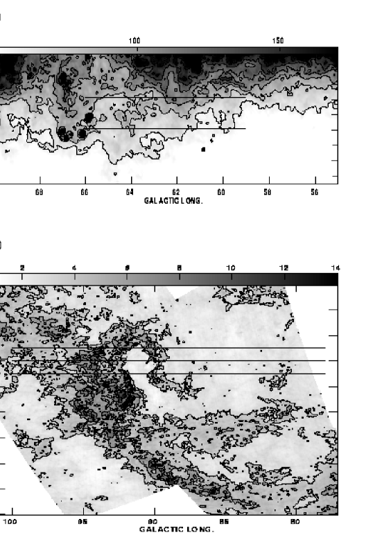
Fig. 1.—: 100 $\rm\mu m$ intensity maps of the Galactic Supershells studied in this paper. The solid lines indicate one-dimensional cuts along which HI 21 cm line observations were made. CO observations were made toward IR-excess regions in these one-dimensional cuts. (a) GS 064$-$01$-$97. Grey-scale varies from 50 to 170 $\rm MJy~{}sr^{-1}$, and contour levels are 60, 80, 100, 120, 140, and 160 $\rm MJy~{}sr^{-1}$. (b) GS 090$-$28$-$17. Grey-scale varies from 1 to 14 $\rm MJy~{}sr^{-1}$, and contour levels are 3.5, 5.5, 7.5, 9.5, 11.5, and 13.5 $\rm MJy~{}sr^{-1}$. (c) GS 174$+$02$-$64. Grey-scale varies from 15 to 50 $\rm MJy~{}sr^{-1}$, and contour levels are 20, 25, 30, 35, and 40 $\rm MJy~{}sr^{-1}$.

Fig. 1.$-$ Continued

CO J=1$-$0 line observations were made using the 14-m telescope (HPBW $\sim 50^{\prime\prime}$) at Taeduk Radio Astronomy Observatory (TRAO) during 1996 March, May, November, and 1997 May. The data were collected using a 256-channel filter bank with a total bandwidth of 64 MHz. The velocity coverage was from $-80$ to $+80\rm~{}km~{}s^{-1}$, and the velocity resolution was 0.65 $\rm km~{}s^{-1}$. The system temperature varied in the range 700$-$1000 K during the observing sessions depending on weather conditions and elevation of the source. The typical rms noise of the spectra was 0.1$-$0.2 K. The antenna temperature was converted to the brightness temperature using a main beam efficiency of 0.39. We first observed IR-excess peaks brighter than 3 MJy $\rm sr^{-1}$ at 100 $\rm{\mu m}$, which is the brightness corresponding to a CO J=1$-$0 line intensity of $\sim 0.1$ K. For the peak positions with detectable CO emission, we have made further observations along the one-dimensional cuts where HI observations had been made. CO spectra were obtained at every $3^{\prime}$ or $4^{\prime}$ using position switching. Observed regions and reference positions are listed in Table 2. The reference positions were checked to have no appreciable ($<0.1$ K) CO J=1$-$0 emission.

III INFRARED EXCESS AND MOLECULAR GAS

(a) HI gas and Infrared excess

Figure 2 shows some representative HI and CO spectra of each object. HI spectra usually have several velocity components, and we integrated over the whole velocity range to derive $N(\rm HI)$ along the line of sight. Assuming that the 21-cm line emission is optically thin, we converted the observed brightness temperature to $N(\rm HI)$.

The method of the analysis was identical to that used in Paper I. First, in each area, we derived the correlation between $N(\rm HI)$ and $I_{100}$, i.e., $I_{100}=a~{}N({\rm HI})+b$. In contrast to Paper I, however, we could not exclude all of the points with detectable CO emission in advance because we did not carry out CO observations toward the whole area. In order to exclude the points with possible molecular gas, therefore, we repeated least-squares fits using only pixels within $\pm 2\sigma$ deviations from the previous fit until the standard deviation did not change. The parameters $a$ and $b$ determined in that way are listed in Table 3. The $I_{100}/N(\rm HI)$ ratios of GS064 and GS090 are consistent with values in the solar neighborhood, while the ratio for GS174 is significantly smaller. Based on the derived relation between $I_{100}$ and $N(\rm HI)$, we can determine the $I_{100}$ excess, i.e., the $I_{100}$ intensity in excess of what would be expected from $N(\rm HI)$. This $I_{100}$ excess can be used to estimate the $\rm H_{2}$ column density;

$$N({\rm H_{2}})_{I_{100}}=\frac{1}{2}\left[\frac{I_{100,c}}{<I_{100,c}/N({\rm H})>}-N(\rm HI)\right]~{}~{}~{}~{}~{}(\rm cm^{-2})$$ (1)

where the subscript ‘c’ indicates the quantity corrected for offset and the angle bracket indicates an average ratio. In this process, we assumed that the dust-to-gas ratios and infrared emissivities of the HI cloud and $\rm H_{2}$ cloud are same. Therefore $<I_{100}/N(\rm H)>$ is equal to $<I_{100}/N(\rm HI)>$.

Table 2.  Positions of scans and OFF positions

		$l/\alpha_{1950}$-range		OFFsa
Name	$b/\delta_{1950}$	HI 21 cm line	CO J=1$-$0 line	($l,b$)/($\alpha,\delta)_{1950}$
GS 064$-$01$-$97
	$-$3$.\!\!^{\circ}$00	66$.\!\!^{\circ}$00$-$59$.\!\!^{\circ}$00	59$.\!\!^{\circ}$75$-$59$.\!\!^{\circ}$45	(59$.\!\!^{\circ}$00,$-$3$.\!\!^{\circ}$00)
			66.00$-$61.55	(60.00,$-3.50$),(63.00,$-4.00$),(65.50,$-4.00$)
	$-2.00$	66.00$-$59.00	59.65$-$59.00	(59.00,$-2.50$)
			62.75$-$60.02	(59.00,$-2.50$)
			65.30$-$63.85	(64.70,$-3.30$)
GS 090$-$28$-$17
	$-$31$.\!\!^{\circ}$00	100$.\!\!^{\circ}$0$-$78$.\!\!^{\circ}$00	94$.\!\!^{\circ}$67$-$91$.\!\!^{\circ}$60	(92$.\!\!^{\circ}$00, $-$31$.\!\!^{\circ}$50),(94.00,$-$30.60)
	$-32.00$	100.0$-$78.00	94.50$-$92.47	(93.00,$-31.50$)
	$-33.00$	100.0$-$78.00	94.33$-$91.93	(91.00, $-33.00$),(95.50,$-33.00$)
GS 174$+$02$-$64
	22$.\!\!^{\circ}$00	${\rm 4^{h}00^{m}00^{s}}$	${\rm 4^{h}07^{m}48^{s}}$$-$${\rm 4^{h}05^{m}24^{s}}$	(${\rm 4^{h}04^{m}12^{s}}$, 21$.\!\!^{\circ}$00)
		$-$${\rm 7^{h}20^{m}00^{s}}$	4 33 00$-$4 19 12	(4 15 00,18.50),(4 30 00,21.50)
			4 45 00$-$4 41 24	(4 43 12,21.50)
			5 21 00$-$5 15 00	(5 18 00,21.00)
			6 18 00$-$5 51 00	(5 30 00,22.00),(6 15 36,21.00)
	24.00	4 00 00	4 34 48$-$4 06 00	(4 04 48,21.00),(4 04 48,23.50),(4 45 00,23.00)
		$-$7 20 00	5 42 00$-$5 30 00	(5 36 00,25.00)
			6 04 48$-$5 52 12	(6 00 00,25.00)

^aOFF positions for CO J=1$-$0 line observations

Fig. 2.—: Representative HI 21 cm (left column) and CO J=1$-$0 (right column) spectra of each object. These are the spectra of the regions where the strongest CO line emission has been detected. The positions are labeled on the upper left part of each picture.

Table 3.  The correlation between $I_{100}$ and $N(\rm HI)$

Name	a	b
	($\rm MJy~{}sr^{-1}~{}(10^{20}~{}cm^{-2})^{-1}$)	($\rm MJy~{}sr^{-1}$)
GS 064$-$01$-$97	1.30 $\pm$ 0.01	$-8.15\pm$0.67
GS 090$-$28$-$17	1.05 $\pm$ 0.02	$-2.00\pm$0.07
GS 174$+$02$-$64	0.40 $\pm$ 0.01	12.13 $\pm$0.18

Note : $I_{100}~{}~{}=~{}~{}aN({\rm HI})~{}+~{}b$

We may alternatively use the 100 $\rm\mu m$ optical depth $\tau_{100}$ for identifying the region with molecular gas. Using 60 and 100 $\rm\mu m$ intensities, we derived the color temperature, $T_{\rm d}$, and $\tau_{100}$. In each area, we determined a mean relation between $\tau_{100}$ and $N(\rm HI)$, and derived the $\tau_{100}$ excess, i.e., the 100 $\rm\mu m$ optical depth in excess of what would be expected from $N(\rm HI)$. This $\tau_{100}$ excess can be used to estimate a separate $\rm H_{2}$ column density;

$$N({\rm H_{2}})_{\tau_{100}}=\frac{1}{2}\left[\frac{\tau_{100,c}}{<\tau_{100,c}/N({\rm H})>}-N(\rm HI)\right]~{}~{}~{}~{}~{}(\rm cm^{-2})$$ (2)

Figures 3$-$5 show the distributions of the derived $T_{\rm d}$, $N({\rm H_{2}})_{I_{100}}$, and $N({\rm H_{2}})_{\tau_{100}}$ in the three supershells. In GS064, the distributions of $N({\rm H_{2}})_{I_{100}}$ and $N({\rm H_{2}})_{\tau_{100}}$ are very similar except at several positions where $N({\rm H_{2}})_{\tau_{100}}$ produces a sharp minimum, e.g., at $(l,b)=($61$.\!\!^{\circ}$3, $-$3$.\!\!^{\circ}$0) and (59$.\!\!^{\circ}$95, $-$2$.\!\!^{\circ}$0). These are the directions toward IRAS point sources with large 60 $\rm\mu m$ fluxes (see Table 4), so that the derived $T_{\rm d}$’s appear sharply peaked. In GS090, the distributions of $N({\rm H_{2}})_{I_{100}}$ and $N({\rm H_{2}})_{\tau_{100}}$ appear similar too. But an important difference is that $N({\rm H_{2}})_{\tau_{100}}$ is greater than $N({\rm H_{2}})_{I_{100}}$ by a factor of $\sim 2.5$. This is consistent with the result of Paper I showing that the $I_{100}$ excess significantly underestimates the amount of molecular gas along the line of sight. Another thing to note is that the areas with large $N({\rm H_{2}})_{\tau_{100}}$ appear to have lower color temperatures, e.g., at $(l,b)=(92^{\circ}-95^{\circ}$, $-31^{\circ}$) and ($92^{\circ}-95^{\circ}$, $-33^{\circ}$). As we show in section III (b), these are the regions with molecular gas. In GS174, we again note that $N({\rm H_{2}})_{\tau_{100}}$ is greater than $N({\rm H_{2}})_{I_{100}}$, particularly at $(\alpha,\delta)=($4$.\!\!\rm^{h}$4$-$4$.\!\!\rm^{h}$6, $24^{\circ}$). However, this the factor is found to vary over the region. There are several positions with very high $T_{\rm d}$’s in GS090 and GS174 too, and they are listed in Table 4.

$N({\rm H_{2}})_{I_{100}}$ would significantly underestimate the molecular content because the IR emissivity of molecular gas, $<I_{100}/N({\rm H})>_{\rm H_{2}}$, could be much lower than that of atomic gas $<I_{100}/N({\rm H})>_{\rm HI}$. In Paper I, we introduced a correction factor

$$\xi_{c}\equiv\frac{<I_{100}/N({\rm H)>_{HI}}}{<I_{100}/N(\rm H)>_{H_{2}}}$$ (3)

that should be applied to $N({\rm H_{2}})_{I_{100}}$ in order to account for the different IR emissivities of molecular clouds. The correction factor could be estimated from $N({\rm H_{2}})_{\tau_{100}}/N({\rm H_{2}})_{I_{100}}$ and, from Figure 3$-$5, we find that $\xi_{c}\simeq 1-1.7$, 2.5, and 3 for GS064, GS090, and GS174. These correction factors, however, are underestimated because $N({\rm H_{2}})_{\tau_{100}}$ is underestimated. Note that one of our assumptions in deriving $N({\rm H_{2}})_{\tau_{100}}$ was a uniform color temperature for dust along the line of sight. But, in general, the 60/100 $\rm\mu m$ color temperature of molecular gas is less than that of atomic gas (see section IV). Therefore, by assuming a uniform color temperature, we overestimate $T_{\rm d}$ and underestimate $\tau_{100}$ (and $N({\rm H_{2}})_{\tau_{100}}$) of molecular gas. The effect becomes greater as the relative amount of atomic gas increases (see Fig. 6 of Paper I). Hence, for the supershells studied in this paper, the effect is largest ($\sim$ 35%) for GS064 where $N({\rm HI})/N({\rm H_{2}})\geq 10$ and the size of this effect is about 20% for the other supershells. If we consider this effect, the true correction factors are $\xi_{c}\simeq 1.5-2.6$, 3.1, and 3.8 for GS064, GS090, and GS174, respectively.

Fig. 3.—: Distributions of (a) $I_{100}$, $N(\rm HI)$, (b) $T_{\rm d}$, (c) $N({\rm H_{2}})_{\tau_{100}}$, $N({\rm H_{2}})_{I_{100}}$, and (d) $W_{\rm CO}$ for GS 064$-$01$-$97. In (a), the thin and thick lines represent $N(\rm HI)$ and $I_{100}$, and, in (c), $N({\rm H_{2}})_{I_{100}}$ and $N({\rm H_{2}})_{\tau_{100}}$. In (d), the thick lines at the bottom indicate the regions where the CO line observations were carried out.

Fig. 4.— Same as Fig. 3 but for GS 090$-$28$-$17.

Fig. 5.— Same as Fig. 3 but for GS 174$+$02$-$64.

Table 4.  Positions with very high $T_{\rm d}$

Name	Positions	IRAS Point Source	Note	Reference
GS 064$-$01$-$97
	(61$.\!\!^{\circ}$30, $-$3$.\!\!^{\circ}$00)	IRAS 19557+2320	External galaxy	1
	(62$.\!\!^{\circ}$15, $-$2$.\!\!^{\circ}$00)	IRAS 19541+2334	?	1
	(59$.\!\!^{\circ}$95, $-$2$.\!\!^{\circ}$00)	…	?
GS 090$-$28$-$17
	(87$.\!\!^{\circ}$60, $-$33$.\!\!^{\circ}$00)	…	?
	(97$.\!\!^{\circ}$40, $-$32$.\!\!^{\circ}$00)	IRAS 23129+2548	?	1
GS 174$+$02$-$64
	(${\rm 5^{h}24^{m}}$37$.\!\!\rm^{s}$8, $21^{\circ}53^{\prime}46^{\prime\prime}$)	…	HD35708 (B2.5IV)	2
	(${\rm 5^{h}31^{m}}$31$.\!\!\rm^{s}$4, $21^{\circ}58^{\prime}54^{\prime\prime}$)	IRAS 05315+2158	Crab supernova remnant	1,4
	(${\rm 4^{h}32^{m}}$31$.\!\!\rm^{s}$5, $24^{\circ}02^{\prime}07^{\prime\prime}$)	IRAS 04325+2402	Young stellar object	1,3
	(${\rm 5^{h}32^{m}}$23$.\!\!\rm^{s}$7, $24^{\circ}00^{\prime}28^{\prime\prime}$)	…	HD36819 (B2.5IV)	2
	(${\rm 5^{h}44^{m}}$45$.\!\!\rm^{s}$5, $24^{\circ}00^{\prime}00^{\prime\prime}$)	IRAS 05447+2400	?	1

REFERENCES.$-$(1) IRAS point source catalog (1988); (2) Gaustad & Van Buren (1993);

(3) Kenyon et al. (1993); (4) Strom & Greianus (1992).

Fig. 6.— $N({\rm H_{2}})_{\tau_{100}}$ vs. $W_{\rm CO}$ (top) and $N({\rm H_{2}})_{I_{100}}$ vs. $W_{\rm CO}$ (bottom) in three supershells . The solid line in each frame represents a least-squares fit to the data .

(b) Comparison of IR excess and CO emission

In Figures 3$-$5, we also show the regions where CO observations have been carried out and the distributions of the CO integrated intensity, $W_{\rm CO}$. If we compare the distributions of either $N({\rm H_{2}})_{I_{100}}$ or $N({\rm H_{2}})_{\tau_{100}}$ with those of $W_{\rm CO}$ in Figure 3, it is obvious that they are correlated. The CO detection rate, i.e., the fraction with detectable CO emission among the observed IR-excess peaks, is very high ($\sim 0.9$) for GS064 while it is 0.7 for GS090 and GS174. $I_{100}$- and $\tau_{100}$-excess peaks have almost the same detection rate. There are, however, $I_{100}$-excess peaks produced by local heating sources instead of molecular gas, e.g., $(\alpha,\delta)=(\rm 5^{h}31^{m}46^{s}$, $22^{\circ}$) and $(\rm 5^{h}32^{m}31^{s}$, $24^{\circ}$) in GS174 (see Table 3). In such regions, which can be identified by their high color temperatures, the $I_{100}$-excess cannot trace the molecular content correctly.

Direct comparison of the $I_{100}$- or $\tau_{100}$-excesses with $W_{\rm CO}$ is not straightforward because the resolution ($50^{\prime\prime}$) of the CO observations is much smaller than those of the HI and IRAS observations. If $W_{\rm CO}$ varies smoothly, however, the comparison could still be useful. Figure 6 compares $N({\rm H_{2}})_{I_{100}}$ and $N({\rm H_{2}})_{\tau_{100}}$ with $W_{\rm CO}$ in three shells. In Figure 6, the solid line represents a least-squares fit to the data and the relation is given in each frame. There are several points to be made from Figure 6. First, in spite of the different beam sizes, there are good correlations between $N({\rm H_{2}})$’s and $W_{\rm CO}$’s. $N({\rm H_{2}})_{\tau_{100}}$ and $N({\rm H_{2}})_{I_{100}}$ have a comparable degree of correlation with $W_{\rm CO}$. But, as we have pointed out in section III (a), their conversion factors $X\equiv N({\rm H_{2}})/W_{\rm CO}$ differ significantly. Second, the conversion factor varies among supershells, i.e., $X=0.26-0.66$, if we use $N({\rm H_{2}})_{\tau_{100}}$. This conversion factor is much smaller than the estimated value for molecular clouds in the Galactic plane, $X=(1.8-4.8)\times 10^{20}~{}\rm cm^{-2}~{}(K~{}km~{}s^{-1})^{-1}$ (Scoville & Sanders 1987), but comparable to that of high latitude clouds, $X\simeq 0.5\times 10^{20}~{}\rm cm^{-2}~{}(K~{}km~{}s^{-1})^{-1}$ (de Vries et al. 1987; Heithausen & Thaddeus 1990; Reach et al. 1998). Some of the molecular gases that we observed in the three supershells comprise parts of previously studied molecular clouds. In GS064, the observed region is the western part of the Cygnus Rift (Dame & Thaddeus 1985). In GS090, it is a part of MBM53 (Magnani, Blitz, & Mundy 1985). In GS174, it covers the southern part of the Taurus complex (Ungerechts & Thaddeus 1987). Third, the fit in GS090 has a large offset, e.g., 3.2 $\rm MJy~{}sr^{-1}$. We consider that this is significant. (GS174 also has a large offset. But since $N(\rm H_{2})$ values are large in GS174, the errors are large. Therefore the large offset in GS174 is not significant.) The large offset, if it is real, implies molecular gas without CO emission. There have been suggestions that diffuse molecular gas would not be observable in CO because CO may not be shielded from UV photons and because CO may not be collisionally excited (van Dishoech & Black 1988; Blitz et al. 1990; Reach et al. 1994; Meyerdierks & Heithausen 1996; Boulanger et al. 1998; Reach et al. 1998). Our result suggests that the critical column density below which the CO line would not be detected is $\sim 3\times 10^{20}~{}\rm cm^{-2}$. This is about half as much as the result of van Dishoech & Black (1988).

IV DISCUSSION

The results of this paper confirm our previous conclusion that there are several shortcomings in using the $I_{100}$ excess for estimating accurate molecular content: First, there are $I_{100}$-excess regions not due to molecular gas but due to high infrared emissivity, e.g., the regions around early-type stars. In this study, the region around Crab in GS174 was such an example, but it was easily discernible by the large color temperature. Second, the $I_{100}$ excess would significantly underestimate the $\rm H_{2}$ column density because of the low infrared emissivity of molecular gas. In the three supershells that we studied, the correction factors are 1.5$-$3.8.

As we have pointed out in Paper I, $\tau_{100}$ and $T_{\rm d}$ are largely affected by small grains. Previous studies showed that 40$-$60% of 60 $\rm\mu m$ emission is contributed by small grains (Sodroski et al. 1994). Hence, $T_{\rm d}$ could be significantly overestimated compared to the equilibrium temperature of large grains. Indeed, this appears to be the case because the derived color temperatures (23$-$25 K) are significantly larger than the mean dust temperatures of the inner (21 K) and outer (17 K) galaxies derived by Sodroski et al. (1994) using the Diffuse Infrared Background Experiment (DIRBE) 140 and 240 $\rm\mu m$ observations. Note that $T_{\rm d}=24$ K when $I_{60}/I_{100}=0.2$ and $T_{\rm d}=21$ K where $I_{60}/I_{100}=0.1$ (e.g., see equation (2) of Paper I). Hence the temperature difference is consistent with the suggestion that $\sim 50\%$ of 60 $\rm\mu m$ emission is contributed by small grains. In this case the 100 $\rm\mu m$ optical depth is underestimated by a factor of $\sim 3$. If the contribution of small dust particles for 60 $\rm\mu m$ emission varies from 10% to 80%, this factor varies from 1.2 to 11.

Our results (in this paper and in Paper I) indicate that $T_{\rm d}$ derived from $I_{60}/I_{100}$ is low in molecular gas. Similar phenomena have been observed in other clouds too (Boulanger et al. 1990; Laureijs et al. 1991; Bernard et al. 1993). $T_{\rm d}$ could be low either because the equilibrium temperature is low or because the abundance of small grains is less, or both. Indeed, the equilibrium temperature of dust grains in molecular gas is lower than that in atomic gas by 2 K (Sodroski et al. 1994). Also, in nearby molecular clouds, it was found that the abundance of small grains decreases in the central regions of molecular clouds (Bernard et al. 1993). Boulanger et al. (1990) suggested that the abundance variation occurs because small grains condense onto grains and do not form in regions of low color ratio, while they are formed and detached from grain mantles in regions of high color ratio.

There have been other suggested methods for estimating the molecular content from $I_{60}$ and $I_{100}$. Laureijs et al. (1991) showed that $\Delta I_{100}\equiv I_{100}-I_{60}/\Theta$, where $\Theta$ is the average value for $I_{60}/I_{100}$ in the outer diffuse region, is strongly correlated with molecular material with densities of $n_{H_{2}}>10^{3}{\rm cm^{-1}}$. Abergel et al. (1994) also found in the Taurus complex that $\Delta I_{100}$ is tightly correlated with $W_{\rm{}^{13}CO}$, and that $\rm{}^{13}CO$-emitting regions coincide with cold regions traced by $\Delta I_{100}$. The DIRBE emission at 140 and 240 $\rm\mu m$ could be also used in calculating $\Delta I_{\lambda}$ (Lagache et al. 1998). These $\Delta I_{\lambda}$ measurements seem to be other good indicators of molecular gas in dense regions. This is probably because $I_{60}/I_{100}$ drops in the molecular cloud due to the combined effect of the decrease in dust temperature and the change in dust properties. Boulanger et al. (1998) introduced $\Delta I_{100}$ multiplied by a scaling factor $\Theta/(\Theta-\Theta_{\rm cold})$, where $\Theta_{\rm cold}$ is the average value for the cold component, to correct for the fraction of 100 $\rm\mu m$ emission from the cold component which is lost in the subtraction. The advantage of this method is that one can search for dense molecular clouds without HI data. We mentioned above the contribution of small grains to $I_{60}$ as major problems in applying the $\tau_{100}$-excess method. On large angular scales, we may use the DIRBE data for the 100, 140, and 240 $\rm\mu m$ wavebands to resolve such problems. In that case, $\tau_{140}$ excess and $\tau_{240}$ excess are recommended as other indicators of molecular gas.

V CONCLUSION

In this paper, we have confirmed our previous results (Kim et al. 1999) suggesting that there are several shortcomings in using the $I_{100}$ excess for estimating accurate molecular content: First there are $I_{100}$-excess regions due to high infrared emissivity, and, second the $I_{100}$ excess would significantly underestimate the $\rm H_{2}$ column density $N(\rm H_{2})$ because of the low infrared emissivity of molecular gas. We may still estimate $N(\rm H_{2})$ from the $I_{100}$ excess by applying the correction factor $\xi_{c}=<I_{100}/N({\rm H)>_{HI}}/<I_{100}/N(\rm H)>_{H_{2}}$, which could be roughly determined from HI and IRAS data. Our results show that $\xi_{c}$ varies from region to region, e.g., $\xi_{c}=1.5$$-$$3.8$ in the three supershells. Therefore, if one applies the $I_{100}$-excess method for deriving an accurate molecular content, the correction factor should be estimated too. An alternative method for estimating molecular content is to use the $\tau_{100}$ excess. In Paper I, we showed that, for the Galactic worm GW46.4+5.5, the $\tau_{100}$ excess had a very good correlation with $W_{\rm CO}$ but the $I_{100}$ excess did not. For the three supershells, however, the difference between the two methods is not as prominent as in GW46.4+5.5. There are several reasons for this: First the $I_{100}$ excess due to high infrared emissivity caused by, e.g., heating by OB stars, is rare at high latitudes and, since the effect is local, it would not significantly affect the correlation between the $I_{100}$ excess and $W_{\rm CO}$ over a large area. Second our observations are biased because we observed only the peak excess positions and the surrounding area. If we had coverd a larger area, the difference might have been more significant.

In conclusion we consider that the $\tau_{100}$-excess method, in general, is a more reliable method for estimating the molecular content than the $I_{100}$-excess method. It might be worthwhile to compare the method with other suggested methods in regions with fully sampled HI and CO data.

ACKNOWLEDGEMENTS This work has been supported in part by the Basic Science Research Institute Program, Ministry of Education, 1997, project BSRI-97-5408.

References

- Abergel, A., Boulanger, F., Mizuno, A., & Fukui, Y. 1994, ApJ, 423, L62
- Bernard, J. P., Boulanger, F., & Puget, J.-L. 1993, A&A, 277, 609
- Boulanger, F., Baud, B. D., & van Albada, G. D. 1985, A&A, 144, L9
- Boulanger, F., & Perault, M. 1988, ApJ, 330, 964
- Boulanger, F., Falgarone, E., Puget, J.-L., & Helou, G. 1990, ApJ, 364, 136
- Boulanger, F., Bronfman, L., Dame, T. M., & Thaddeus, P. 1998, A&A, 332, 273
- Blitz, L., Bazell, D., & Désert, F. X. 1990, ApJ, 352, L13
- Désert, F.X, Bazell, D., & Boulanger, F. 1988, ApJ, 334, 815 (DBB)
- de Vries, H. W., Heithausen, A., & Thaddeus, P. 1987, ApJ, 319, 723
- Gaustad, J. E., & van Buren, D. 1993, PASP, 105, 1127
- Heiles, C. 1979, ApJ, 229, 533
- Heiles, C. 1984, ApJS, 55, 585
- Heiles, C., Reach, W. T., & Koo, B.-C. 1988, ApJ, 332, 313
- Heithausen, A., & Thaddeus, P. 1990, ApJ, 353, L49
- Heithausen, A., Stacy, J. G., de Vries, H. W., Mebold, U., & Thaddeus, P. 1993, A&A, 268, 265
- IRAS Point Source Catalog, Version 2, 1988, Joint IRAS Science Working Group (Washington, DC:GPO)
- Kenyon, S. J., Calvet, N., & Hartmann, L. 1993, ApJ, 414, 676
- Kim, K.-T., Lee, J.-E., & Koo, B.-C. 1999, ApJ, in press (Paper I)
- Koo, B.-C., Reach, W. T., & Heiles, C. 1990, ApJ, 364, 178
- Lada, E. A., & Blitz, L. 1988, ApJ, 326, L69
- Lagache, G., Abergel, A., Boulanger, F., & Puget, J.-L. 1998, A&A, 333, 709
- Laureijs, R. J., Clark, F. O., & Prusti, T. 1991, ApJ, 372, 185
- Low, F. J., et al. 1984, ApJ, 278, L19
- Magnai, L., Blitz, L., & Mundy, L. 1985, ApJ, 295, 402
- Mathis, J. S., Mezger, P. G., & Panagia, N. 1983, A&A., 128, 212
- Meyerdierks, H., & Heithausen, A. 1996, A&A, 313, 929
- Reach, W. T., Koo, B.-C., & Heiles, C. 1994, ApJ, 429, 672
- Reach, W. T., Wall, W. F., Odegard, N. 1998, ApJ, 507, 507
- Scoville, N. Z., & Sanders., D. B. 1987, in Interstellar Processes, ed. D. Hollenbach, & H. Thronson (Dordrecht: D. Reidel), 21
- Sodroski, T. J., et al. 1994, ApJ, 428, 638
- Strom, R., G., & Greidanus, H. 1992, Nature, 358, 654
- Ungerechts, H., & Thaddeus, P. 1987, ApJ, 63, 645
- van Dishoeck, E. F., & Black, J. H. 1988, ApJ, 334, 771