The specific entropy of elliptical galaxies: an explanation for profile-shape distance indicators?

Abstract

Dynamical systems in equilibrium have a stationary entropy; we suggest that elliptical galaxies, as stellar systems in a stage of quasi-equilibrium, may have in principle a unique specific entropy. This uniqueness, a priori unknown, should be reflected in correlations between the fundamental parameters describing the mass (light) distribution in galaxies. Following recent photometrical work on elliptical galaxies (Caon et al. 1993; Graham & Colless 1997; Prugniel & Simien 1997), we use the Sérsic law to describe the light profile and an analytical approximation to its three dimensional deprojection. The specific entropy is then calculated supposing that the galaxy behaves as a spherical, isotropic, one-component system in hydrostatic equilibrium, obeying the ideal gas state equations. We predict a relation between the 3 parameters of the Sérsic law linked to the specific entropy, defining a surface in the parameter space, an ‘Entropic Plane’, by analogy with the well-known Fundamental Plane. We have analysed elliptical galaxies in two rich clusters of galaxies (Coma and ABCG 85) and a group of galaxies (associated with NGC 4839, near Coma). We show that, for a given cluster, the galaxies follow closely a relation predicted by the constant specific entropy hypothesis with a typical dispersion (one standard deviation) of 9.5% around the mean value of the specific entropy. Moreover, assuming that the specific entropy is also the same for galaxies of different clusters, we are able to derive relative distances between Coma, ABGC 85, and the group of NGC 4839. If the errors are only due to the determination of the specific entropy (about 10%), then the error in the relative distance determination should be less than $20\%$ for rich clusters. We suggest that the unique specific entropy may provide a physical explanation for the distance indicators based on the Sérsic profile put forward by Young & Currie (1994, 1995) and recently discussed by Binggeli & Jerjen (1998).

1 Introduction

Elliptical galaxies are believed to be self-gravitating systems in a quasi-equilibrium state. They are far from being the simple, dull objects they were thought to be until the early 70’s: high spatial and spectroscopic observations have revealed that elliptical galaxies show a great variety of fine structures (e.g. Kormendy 1984, Bender & Möllenhoff 1987). However, underlying these fine structures, elliptical galaxies have a striking regularity concerning their radial light distribution. Indeed, until the mid 80’s, it seemed that the brightness profile of elliptical galaxies could be well described by the de Vaucouleurs (1948) $R^{1/4}$ law (e.g. Kormendy 1977). Nevertheless, systematic departures from the $R^{1/4}$ law were observed (Michard 1985; Schombert 1986, 1988) and, more recently, thanks to higher quality observations, it was shown (Caon et al. 1993; Graham & Colless 1997) that elliptical galaxies in a very wide range of sizes can be well modelled by the Sérsic (1968) empirical law (expressed in magnitude):

$$\mu=\mu_{0}+k_{n}(\frac{R}{R_{{\rm eff}}})^{(1/n)}$$ (1)

a non-homologous generalization of the $R^{1/4}$ law. $\mu_{0}$ is the central brightness, $R_{{\rm eff}}$ is the effective radius and $k_{n}$ a function depending on $n$ (see below, §3.1).

Besides the light profile, another very important regularity observed in elliptical galaxies is the so-called Fundamental Plane (Dressler et al. 1987b; Djorgovski & Davis 1987). Elliptical galaxies populate a two dimensional surface in the three dimensional space defined by the effective radius, $R_{\rm eff}$, the mean surface brightness inside this radius, $\langle\mu\rangle_{\rm eff}$, and the central line of sight velocity dispersion, $\sigma_{0}$. The understanding of such a relation should provide important clues to the formation and evolution of these galaxies.

What is the origin of the relations among the parameters describing the light (and mass) distributions of elliptical galaxies? If these objects are, as we believe, in equilibrium, then the virial theorem should apply and we can derive for a given mass distribution a relation among the gravitational radius, total mass, and mean velocity dispersion. This relation can be ‘translated’ in the observed Fundamental Plane with the help of some hypotheses related to the mass to light ratio, light distribution, and hydrostatic equilibrium (Bender et al. 1992, Ciotti & Lanzoni 1997). The validity of these hypotheses is, however, still a matter of debate (cf. for instance Prugniel & Simien 1997).

Other than its theoretical importance, the scaling relations of the fundamental parameters of galaxies may have a practical application as a distance indicator. Thus, like the Fundamental Plane (Djorgovski & Davis 1987), the $D_{n}$–$\sigma$ relation (Dressler et al. 1987a), Tully & Fisher (1977) method for spiral galaxies, etc., the parameters of the Sérsic law can also be used to derive distances (Young & Currie 1994, 1995).

In this paper we will look for fundamental relations among the parameters describing the light distribution of elliptical galaxies. The starting point is also the fact that these galaxies are in equilibrium, but we will use the maximum entropy postulate of thermodynamics instead of the virial theorem. We will derive an expression relating the free parameters of the Sérsic profile to the specific entropy. We will also give a number of useful and simple expressions to calculate the astrophysical quantities related to the Sérsic profile and its three dimensional deprojection. We will then show that the specific entropy relation holds for at least two clusters of galaxies and we suggest that it may, in principle, be used as a relative distance indicator like the shape-profile distance indicators introduced by Young & Currie (1994, 1995).

2 The entropy

2.1 Thermodynamics

The regularity observed in the light distribution of elliptical galaxies may be conveniently understood as an evolutionary convergence. Independently of the initial conditions, these galaxies evolve towards a single class of objects. Since the stellar two-body relaxation time scale is far greater than the age of the Universe, the mechanism behind this evolution is probably the so-called violent relaxation (Lynden-Bell 1967). The rapidly changing global gravitational potential (due to an initial collapse or merging) produces a mixing in phase space within the same time scale as the collapse or merging itself.

The second postulate of thermodynamics says that, when a dynamical system is in equilibrium, then this system is in a state of maximum entropy. If, for a given system, there exists only one state of thermodynamic equilibrium that can be reached, independently of the initial conditions, then it is associated with a stable state of single, global maximum entropy. Gravitational systems, however, present some difficulties: given an arbitrary isolated, self-gravitating system of point particles, the entropy can grow indefinitely by collapsing part of the mass in the centre and expanding the outer parts to infinity, while still conserving the total mass and energy. This is the gravo-thermal catastrophe which can actually occur because a gravitational system has negative specific heat (Lynden-Bell & Wood 1968; Saslaw 1985).

Thus, if we try to maximise the entropy (requiring that the mass and energy be constant) in order to get the equilibrium (and hopefully stable) configuration, we obtain an isothermal sphere (Lynden-Bell & Wood 1968), which does not match the observed elliptical galaxies. A lot of work has been done these last three decades to obtain the structure of self-gravitating systems from the maximum entropy principle (e.g. Antonov 1962; Lynden-Bell 1967; Shu 1978; Binney 1982; Tremaine et al. 1986; Dejonghe 1987; Richstone & Tremaine 1988; Merritt et al. 1989; Spergel & Hernquist 1992; Hjorth & Madsen 1995). A local maximum entropy can be found if some ad hoc constraints are imposed (e.g. imposing a power law density profile, White & Narayan 1987).

Here, we adopt a different approach: we just assume the existence of a local maximum entropy associated with the elliptical galaxies, without trying do obtain this entropy from first principles. Except for interacting galaxies, it is reasonable to suppose that elliptical galaxies are, at least, objects in thermodynamic quasi-equilibrium (the best evidence being the regularity in the luminosity distribution). Hence, we will proceed computing the entropy of a self-gravitating system using classical thermodynamics. Let us assume that the stars in a galaxy behave like an isolated, self-gravitating gas of equal mass particles. Consequently, we start by taking the differential of the entropy:

$${\rm d}S=\frac{1}{T}{\rm d}E+\frac{P}{T}{\rm d}V-\frac{\mu_{q}}{T}{\rm d}N\,,$$ (2)

where $S,E,V,N,T,P,\mu_{q}$ are, respectively, the entropy, energy, volume, number of particles, temperature, pressure, and chemical potential. Formula (2) is nothing more than the fundamental equation of thermodynamics (also know as the Euler relation) in the entropy representation (e.g. Callen 1960), which applies to any thermodynamic system in equilibrium. For an isolated, self-gravitating system, the extensive and intensive parameters in Eq. (2) are usually interpreted using their classical meaning. For instance, the chemical potential $\mu_{q}$ (that appears already in the work of Lynden-Bell 1967 in the context of stellar dynamics) gives the variation rate of the energy with the number of particles, ${\rm d}E/{\rm d}N$, for constant entropy and volume (see also Saslaw 1985) or, from the statistical physics point of view, $\mu_{q}$ is related to the Fermi energy of the system (Stiavelli 1998). The temperature is defined in terms of the velocity dispersion $\sigma$, as $kT=m\sigma^{2}$ ($m$ is the mean particle mass of the system).

We now need the equations of state in order to describe the properties of the ‘gas’ of stars. There is no known exact equation of state for a gas of self-gravitating particles, so we will use the ideal gas equations which are usually a good approximation for hot, structureless, rarefied gases:

$$E = {3\over 2}N\;kT\;;\quad PV=N\;kT\;;$$

$$\mu_{q} = kT\ln\left({{N\over V}{\left[{{h^{2}\over 2\pi m\;kT}}\right]}^{3/2}}\right)\,,$$ (3)

where $k$ and $h$ are the Boltzmann and Planck constants. Although the above equations of state are a good approximation for non-interacting, mono-atomic, hot gas (in fact, these equations violate the third law of thermodynamics or Nernst postulate, i.e. that the $S\rightarrow 0$ as $T\rightarrow 0$), their application for interacting particles is doubtful. Modifications of the Eqs. (3) have been proposed; Bonnor (1956, and references therein) discusses a modification of Boyle’s Law that takes self-gravity into account. However, that modification was derived for a bounded, isothermal sphere and it adds considerable complication to the problem without really putting away the simplifying hypotheses. Therefore, we take a pragmatic approach and we will use the simplest physically acceptable equations of state, Eqs. (3). The validity or not of our approach should be verified a posteriori.

Thus, we can now write the entropy as a function of the mass density $\rho=mN/V$ and pressure $P$. Using Eq. (2) and Eqs. (3), we obtain, after straightforward algebra:

$${m\over k}{{\rm d}S\over{\rm d}V}={5\over 2}\rho+\rho\ln\left({\rho^{-5/2}\;P^{3/2}\left({{2\pi\over h^{2}}}\right)m^{4}}\right)\,.$$ (4)

We now define the specific entropy $s\equiv S/M$, where $M$ is the total mass of the system. Therefore we write:

$$s={1\over M}\int_{V}\ln\left({\rho^{-5/2}\;P^{3/2}}\right)\rho\,{\rm d}V+\mbox{constant}\,,$$ (5)

where the ‘constant’ above does not depend on the density distribution and we will drop it hereafter. Notice that the above equation is the same used by White & Narayan (1987). Equation (5) can be written in a more compact form using the definition of a mean value, $\langle x\rangle=\int xf(x){\rm d}x/\int f(x){\rm d}x$, and interpreting the density $\rho$ as a distribution function:

$$s=\left\langle{\ln\left({\rho^{-5/2}\;P^{3/2}}\right)}\right\rangle\,.$$ (6)

In Appendix 1 we show that we can obtain the same form for the specific entropy as in Eq. (6) using the Boltzmann-Gibbs definition of the entropy.

2.2 Entropy and light profile

The parameters needed for the evaluation of the specific entropy of early type galaxies are not accessible by direct observation. The calculation of the specific entropy must thus be obtained using the available light profile and some additional hypotheses.

It is clear that, to calculate the mass distribution needed to compute the specific entropy of the galaxy from the observed light distribution, we will need to introduce a mass-to-luminosity ratio, $M/L$. In general, the radial variation of the $M/L$ ratio in elliptical galaxies is poorly known, basically because its determination depends on knowledge of the intrinsic shape and detailed dynamics of the galaxy. So far, there is little evidence for radial gradients of $M/L$ up to $2R_{\rm eff}$ (de Zeeuw 1992, Bertin et al. 1994, Carollo et al. 1995, Rix et al. 1997).

Therefore, we suppose that the galaxy behaves like a one-component system. This means that either (I) the stellar component is dominant (the invisible matter is negligible), or (II) the luminous and dark matters are distributed in the same manner, or else (III) the dark matter has a very extended distribution, being flat and less important than the visible component in the central region (it is the case if the luminous part of an elliptical galaxy is embedded in a very large dark matter halo).

The velocity dispersion tensor is not a priori isotropic in a galaxy, so that the radial and transverse velocity dispersions may not always be equal (for a discussion see Binney & Tremaine 1987). Moreover, normal elliptical galaxies are known to have little rotation (cf. de Zeeuw & Franx 1991 and references therein). We suppose therefore, when using the equations of state (3), that the gas of stars is actually isotropic and with null angular momentum. This simplification will enable us to calculate the pressure of the gas of stars without adding any other parameter to the problem.

The next step for really computing the entropy is to determine the radial mass distribution of galaxies.

3 The Sérsic law

3.1 Generalities

A generalization of the de Vaucouleurs profile has been proposed by Sérsic (1968), Eq. (1). His profile has been widely used in recent years for modelling and theoretical studies of elliptical galaxies (e.g., Ciotti 1991; Caon et al. 1993; Colless & Dunn 1996; Courteau et al. 1996; Prugniel & Simien 1997; Graham et al. 1996; Graham & Colless 1997). The Sérsic law is one of the most compact and simple expressions that describes very precisely the light distribution in a wide range of early-type galaxies.

Instead of the historical form of the Sérsic law, Eq. (1), we will use throughout this paper the following mathematically more compact and natural form:

$$\Sigma(R)=\Sigma_{0}\exp(-(R/a)^{\nu})\,.$$ (7)

Sometimes we call it the $\nu$-model, by analogy to the $\beta$-model (very often used to describe the x-ray profiles of galaxy clusters).

The Sérsic profile is characterised by a normalisation parameter, $\Sigma_{0}$; a scale length, $a$; and a structural (or shape) parameter, $\nu$ ($\nu\equiv 1/n$). The de Vaucouleurs profile is of course equivalent to $\nu=0.25$. We call $\nu$, $a$, and $\Sigma_{0}$ the primary parameters of the Sérsic law.

From the mathematical point of view, the Sérsic profile primary parameters are naturally independent, i.e. if – as we will show later – after a fit, some correlation among these parameters occurs, it will be only due to physical properties. This is not the case when other kinds of parameters such as effective radius or effective brightness are used, because they involve combinations (usually non linear) of the primary parameters (cf. Gerbal et al. 1997 and the end of §5). Such parameters we call the secondary parameters of the Sérsic law.

We will now give some quantities of astrophysical interest and/or useful for the present paper. Calculations are generally straightforward or are presented in the Appendix 2. For the sake of simplicity, we will often give approximate but analytical expressions for these quantities. The analytical approximations are obtained by fitting convenient simple functions to the exact values computed numerically. We will refer to the accuracy of the analytical approximations of a given quantity $\zeta$ in terms of $(\zeta_{\rm theo}-\zeta_{\rm app})/\zeta_{\rm theo}$, where $\zeta_{\rm theo}$ is the exact theoretical value and $\zeta_{\rm app}$ is the analytical approximation. Notice that we do not use the calculations provided by Ciotti (1991), since he based his calculations on a numerical deprojection of the Sérsic law while we use an analytical approximation described below.

The total luminosity inside the radius $R$ is readily obtained by integrating the profile given in Eq. (7):

$$L(R)=\frac{2\pi a^{2}}{\nu}\;\Sigma_{0}\;\hbox{\Large$\gamma$}\!\left(\frac{2}{\nu},\left(\frac{R}{a}\right)^{\nu}\right)\,,$$ (8)

where $\gamma(b,x)$ is the standard incomplete gamma function. The total luminosity is, then,

$$L_{{\rm tot}}=a^{2}\;\Sigma_{0}\;L^{*}(\nu)\,,$$ (9)

where $L^{*}(\nu)\equiv 2\pi\Gamma(2/\nu)/\nu$ and $\Gamma(x)$ is the complete gamma function.

The total magnitude, $m_{\rm tot}=-2.5\log L_{\rm tot}+$ constant, can be obtained accurately (better than 0.5%) for $0.1\leq\nu\leq 2.0$ by the following analytical approximation:

$$m^{*}(\nu)=-0.304\nu-1.708\nu^{-1.44}\,,$$ (10)

with $m^{*}(\nu)\equiv-2.5\log L^{*}(\nu)$.

The effective brightness, $\mu_{\rm eff}$, is the brightness at the effective radius, $R_{\rm eff}$ (defined as the radius having half the total luminosity inside it), i.e. $\mu_{\rm eff}=\mu(R_{\rm eff})$, and is given by (within 0.5% accuracy):

$$\mu_{\rm eff}=-2.5\log\Sigma_{0}+1.0857(R_{\rm eff}/a)^{\nu}\,.$$ (11)

The mean surface brightness inside $R_{\rm eff}$ can be written, by definition, as:

$$\langle\mu\rangle_{\rm eff}=m^{*}+5\log(R_{{\rm eff}}/a)-2.5\log\Sigma_{0}+2.5\log(2\pi)\,.$$ (12)

The effective radius, $R_{{\rm eff}}$, is obtained by solving numerically the equation $2\gamma(2/\nu,(R/a)^{\nu})=\Gamma(2/\nu)$. We have derived an analytical approximation given by:

$$\ln(R_{{\rm eff}}/a)=\frac{0.6950-\ln(\nu)}{\nu}-0.1789\,,$$ (13)

which is accurate to better than 0.6% in the range $0.1\leq\nu\leq 1.8$ for $R_{{\rm eff}}/a$.

Another useful quantity is the Petrosian metric radius, which is related to the logarithm slope of the brightness profile (Petrosian 1976). The Petrosian radius is defined with the help of the variable

$$\eta=-2.5\log\left(\frac{{\rm d}\log L(R)}{2{\rm d}\log R}\right)=\mu(R)-\langle\mu(R)\rangle\,,$$ (14)

where $\mu(R)$ is the magnitude (equal to $-2.5\log(\Sigma)$) at $R$ and $\langle\mu(R)\rangle$ is the mean magnitude inside $R$ (Sandage & Perelmuter 1990). For a given value of $\eta$, a radius $R_{p}$ is defined. Besides being model independent, the Petrosian radius gives a metric measure that is distance independent. For the particular case where $R_{p}=R_{{\rm eff}}$, the Petrosian parameter $\eta$ is a function of $\nu$ given approximately by:

$$\eta=0.6213-1.25\log(\nu)+0.07656\nu\,,$$ (15)

which is valid in the range $0.1\leq\nu\leq 1.8$ with an accuracy of 0.1%.

As we mentioned before, almost all ‘astrophysical’ quantities such as the effective radius, the effective brightness and the mean effective brightness are non-linear combinations of the ‘primary parameters’ $\Sigma_{0}$, $a$ and $\nu$.

It is also interesting to rewrite the Sérsic profile (Eq. 7) introducing explicitly the effective Radius:

$$\Sigma(R)=\Sigma_{0}\exp\left[-b_{\nu}(R/R_{\rm eff})^{\nu}\right]\,,$$ (16)

with $b_{\nu}=(R_{\rm eff}/a)^{\nu}$. The original Sérsic profile, Eq. (1), is obtained making $k_{n}=1.0857b_{\nu}$ and $\mu(R)=-2.5\log\Sigma(R)$.

3.2 Three dimensional Sérsic deprojection

The two dimensional Sérsic density distribution has no analytical deprojection in three dimensions. For our purposes, numerical deprojection (cf. Young 1976 for the de Vaucouleurs case) or the asymptotic behaviour (Ciotti 1991) of the Sérsic profile are not well adapted. Mellier & Mathez (1987) have given a simple analytical approximation of the deprojection of the de Vaucouleurs profile; we will use a modified form of the Mellier & Mathez three dimensional density profile, generalised for the Sérsic profile case:

$$\rho(r)=\rho_{0}{\left({{r\over a}}\right)}^{-p}\exp\left({-{\left({{r\over a}}\right)}^{\nu}}\right)\,,$$ (17)

with the normalisation:

$$\rho_{0}=\Sigma_{0}\frac{\Gamma(2/\nu)}{2a\Gamma((3-p)/\nu)}\frac{M}{L}\,,$$ (18)

which is obtained by requiring that both total masses corresponding to Eqs. (7) and (17) be equal. $M/L$ is the mass to luminosity ratio and we suppose hereafter that it is independent of the galaxy radius. This is the above mentioned hypothesis (§2.2) that the galaxy behaves like a one component system. Notice, however, that up to this point we do not require that all galaxies have the same $M/L$ ratio.

The exponent $p$ in Eq. (17) is obtained by fitting the (numerical) Abel deprojection of the two dimensional profile Eq. (7) to the analytical three dimensional profile Eq. (17). A high quality match, better than 5%, between the numerical deprojection of Eq. (7) and Eq. (17) is obtained when:

$$p=1.0-0.6097\nu+0.05463\nu^{2}\,,$$ (19)

for $0.1\leq\nu\leq 1.8$, and the radial range $10^{-2}\leq R/R_{{\rm eff}}\leq 10^{3}$. The discrepancy between the numerical and analytical deprojections is more pronounced for very small and very large radii. Prugniel & Simien (1997) proceeded in the same fashion, using a modification of the Mellier & Mathez profile, but their deprojection is only valid in the range $0.1\leq\nu\leq 0.5$. Within this range their result and ours agree well within 1%. For $0.5\leq\nu\leq 1$ our result is within 5% to Prugniel & Simien’s, while for $\nu>1$, our result diverges parabolically from theirs.

Notice that the behaviour of Eq. (17) as $r\rightarrow 0$ is not the same as the exact Abel deprojection of the Sérsic profile. For small radii, $\rho_{Abel}(r)\propto r^{\nu-1}$ for $\nu<1$. This should not introduce any appreciable error in our analytical approximation; the fraction of mass inside $10^{-2}\leq R/R_{{\rm eff}}\leq 10^{3}$ is 97% for $\nu=0.1$, 99.6% for $\nu=0.25$, and greater than 99.9% for $\nu\geq 0.55$.

The corresponding mass inside the radius $r$, $M(r)$, is readily obtained integrating Eq. (17) in a spherical volume:

$$M(r)=\frac{4\pi\;\rho_{0}a^{3}}{\nu}\gamma\left(\frac{3-p}{\nu},\left(\frac{r}{a}\right)^{\nu}\right)\,.$$ (20)

Additionally, we give the relation between the two dimensional half-mass radius $R_{{\rm eff}}$ and the three dimensional half-mass radius, $r_{{\rm eff}}$, as a polynomial approximation:

$$r_{{\rm eff}}/R_{{\rm eff}}=1.356-0.0293\nu+0.0023\nu^{2}\,,$$ (21)

This approximation agrees well within 0.25% to the values computed by Ciotti (1991) who used the numerical Abel inversion of the Sérsic profile. This reassures us on the quality of Eq. (17).

We define a gravitational radius by the relation $r_{g}\equiv GM^{2}/|U|$, with $U$ the gravitational potential energy. Again, we give a simple analytical approximation:

$$\ln(r_{g}/a)=0.845+\frac{0.820-0.924\ln(\nu)}{\nu}\,,$$ (22)

that is accurate to better than 0.8% in the range $0.1\leq\nu\leq 1.8$ for $r_{g}/a$. This radius is a combination of the natural scale length and the form factor; this is naturally due to the loss of homology when moving from a de Vaucouleurs law to a $\nu$-model. A similar behaviour occurs with $R_{\rm eff}$, Eq. (13). It turns out that the relation between $R_{\rm eff}$ and $r_{g}$ is roughly linear, independent of $\nu$, given approximately by

$$\ln(r_{g}/a)=1.16+0.98\ln(R_{\rm eff}/a)\,,$$ (23)

accurate to better than 5% in the range $0.1\leq\nu\leq 1.8$ for $r_{g}/a$. For $0.15\leq\nu\leq 1.0$, the relation is practically linear (within 15%), viz. $r_{g}\approx 3.0R_{\rm eff}$ – an interesting result given that the Sérsic model is not homologous.

3.3 Entropy and the Sérsic profile

Given a mass distribution law, the deprojected Sérsic law, we can make the connection between the specific entropy and the parameters of the light profile. We need, however, an additional hypothesis to get the pressure corresponding to Eq. (17). We consider that the pressure is isotropic and the galaxy is in hydrostatic equilibrium. This implies an isotropic velocity dispersion tensor and the simple relation, $P(r)=\rho(r)\sigma_{r}^{2}$, relating the pressure, density, and radial velocity dispersion, $\sigma_{r}$. With the isotropy hypothesis, $\sigma_{r}$ (or $P(r)$) is, thus, obtained as a solution of the hydrostatic equilibrium equation:

$${{\rm d}\over{\rm d}r}\left[\rho(r)\;\sigma_{r}^{2}(r)\right]=-{G\;M(r)\;\rho(r)\over r^{2}}\,,$$ (24)

With the above hypothesis, one may substitute the density and pressure in Eq. (6) and a relation of the kind $s(a,\Sigma_{0},\nu)$ can be derived. It turns out that $s(a,\Sigma_{0},\nu)$ may be well approximated by the analytical expression:

$$s(a,\Sigma_{0},\nu) = {1\over 2}\ln(\Sigma_{0})+{5\over 2}\ln(a)$$ (25)

$$+ c_{1}\ln(\nu)-\frac{1}{\nu}+c_{2}\nu^{c_{3}}+c_{0}\,.$$

The constants $c_{i}$ as well as the derivation of Eq. (25) are given in Appendix 2.

It is interesting to note that for a Plummer profile (polytrope of index 5, e.g. Binney & Tremaine 1987), where we are able to compute exactly the specific entropy, we have the same dependency of $s$ on the Plummer scale and normalisation parameters as in Eq. (25).

The relations that can be written as the formal expression

$$s(a,\Sigma_{0},\nu)=s_{i}\,,$$ (26)

where $s_{i}$ means any given value of the specific entropy, define a family of surfaces in the three dimensional space defined by the parameters $\Sigma_{0}$, $a$, $\nu$. By analogy with the Fundamental Plane, we call such a surface the ‘Entropic Plane’.

We do not know a priori the value of the specific entropy. We can, nevertheless, propose two hypotheses concerning the entropy of elliptical galaxies:

• Hypothesis I: The specific entropy of early-type galaxies in a given cluster is constant. This is the weak hypothesis.

• Hypothesis II: The specific entropy of early-type galaxies in clusters is universal, independent of the cluster in which they are located. This is the strong hypothesis.

One may hope that in the future, some theory of galaxy formation will move one of the two hypotheses above into a firm knowledge and provides us with the true value of $s$. In the absence of a way to calculate $s$ from first principles, these hypotheses must be tested using the observed brightness profiles of early type galaxies.

4 The data

In order to verify these hypotheses, we use the brightness profile data of elliptical galaxies belonging to two rich clusters of galaxies – Coma and ABCG 85 – and the group associated with NGC 4839 (which is in the neighbourhood of Coma).

4.1 Description

Galaxies in the Coma cluster have been selected from the catalogue of Biviano et al. (1995a) among those in the centre of the cluster and in the group around NGC 4839, being brighter than 17.8 $V$ mag, fainter than 13 $V$ mag (to exclude the biggest, saturated galaxies), with elliptical morphological types as assigned by Godwin, Metcalfe & Peach (1983, hereafter GMP), and with measured redshifts that confirm them as cluster members (radial velocity in the range 3000–10000 km s^-1, cf. Biviano et al. (1995b)). The elliptical galaxies of ABCG 85 were extracted from the catalogue of Slezak et al. (1998), by selecting those galaxies belonging to the cluster (from available redshifts, with velocities in the range 13350–20000 km s^-1, cf. Durret et al. (1998)) and with elliptical appearance in the CCD images. The final list of elliptical galaxies used for the fitting is given in Tables 1, 2, and 3 (in their first columns we give the corresponding identifications in both catalogues, Biviano et al. 1995a for Coma and the NCG 4839 group, and Durret et al. 1998 for ABCG 85).

We have used $V$ images that had been reduced and calibrated following standard techniques (see Lobo et al. 1997, Slezak et al. 1998). We then cleaned the images by eliminating foreground stars that contaminated our target galaxies. This was made through specific tasks within IDL (Interactive Data Language, Research Systems, Inc.). The elimination was done by interpolating the field around the star by a 4th degree polynomial. We then obtained the growth curves (integrated magnitudes within circular regions) by means of the ‘ellipse’ task in ‘stsdas’ environment of iraf. For every galaxy in our sample we obtained a table listing the radii of the circular apertures and the corresponding integrated magnitudes inside the apertures. Galaxies that had less than nine data points were rejected. This means that the galaxies on the faint surface brightness end were rejected by our selection. Since our analysis is not sensitive to the completeness of the sample, the rejection of very faint galaxies should have no effect in our results.

The use of a circular aperture was motivated by two reasons. First, in order to be able to compare directly our results with those found in the literature, in particular Graham & Colless (1997) and, second, because the theory we developed is based on spherical symmetry of the mass distribution. Notice that previously (Gerbal et al. 1997) we have employed a different method for obtaining the growth curves, taking into account the shape of the isophotes (we computed the total luminosity inside a given isophote). Comparing our previous results (Figs. 1 and 2 from Gerbal et al. 1997) with those presented here shows that the difference is not significant (i.e., the pairwise distributions of the Sérsic parameters do not change).

4.2 The fitting method

We have fitted the resulting luminosity growth curves of the elliptical galaxies in Coma (including the group of NGC 4839) and ABCG 85.

The advantage of fitting the integrated flux instead of the luminosity profile is that the latter is more sensitive to irregularities in the light distribution. Besides, fitting the light growth curve gives more weight to the inner than the outer parts of the galaxy, reflecting better the galaxy overall structure (D’Onofrio & Prugniel 1997). Therefore, since the inner region of a given galaxy is probably more relaxed than the outer region (which is more susceptible to perturbations) it seems more reasonable to give more weight to the inner region when computing the specific entropy. The drawback is that if the galaxy has some unusual centre, an active nucleus, star burst or some exceptional darkening, then these features will be propagated in the whole growth curve. In this case, fitting the luminosity profile would be better to subtract the anomalous central contribution (D’Onofrio & Prugniel 1997). Moreover, Burstein et al. (1987) pointed out that the fitting of growth curve have systematic uncertainties that may lead to correlated errors of the total magnitude and the effective radius. This last point may be minimized by fitting the uncorrelated primary parameters of the Sérsic law (cf. §3.1) rather than their non linear combinations.

Consequently, we use the integrated form of the brightness profile as given by Eq. (8). The luminosity growth curve fits are done with a standard least square minimisation method, using the ‘minuit’ programme from the CERN software library. In order to reduce the effects of the seeing (FWHM $\approx 0.9$ arcsec for Coma and 1.2 arcsec for ABCG 85) and/or eventual nuclear activity, the data points are taken only from 2.5 arcsec outwards. For galaxies of the same cluster, the effect of using a central exclusion mask fixed in angular units, rather than a linear measure, is virtually negligible (in this precise case the galaxies can be considered to be at the same distance from us; for Coma the error should be smaller than $\sim 5$%). A difficulty may rise in comparing galaxies in different clusters. However, in our case, the clusters are not more than a factor 2.5 apart (radial distance; cf. §6 below) and changing the size of the mask from 0.6 to 3.0 arcsec did not alter significantly the fitting results, i.e., the values obtained for the Sérsic parameters were compatible within their 3$\sigma$ error bars [notice that this test on the size of the central mask were also done by Gerbal et al. (1997)].

We have used the growth curve up to the surface brightness isophote at $24.0\;V$ mag/arcsec², corresponding to a 3$\sigma$ signal above the background sky. This is done in order to minimize errors introduced in the background subtraction. We performed the fits varying the outer cut-off from 22.5 to 24.5 $V$ mag/arcsec²; the fitting results were still basically the same, i.e., the values obtained for the Sérsic parameters were compatible within their 3$\sigma$ error bars.

Table 1: Growth curve fitting results for Coma. Ident is the GMP number and name is either an IC or NGC identification. $\nu$ and $a$ are the shape and scale parameters fitted with the Sérsic law. $\mu_{0}=-2.5\log(\Sigma_{0})$ is the intensity parameter and the magnitude is in the $V$ band. $R_{{\rm eff}}$ and $\langle\mu\rangle_{{\rm eff}}$ are calculated from the primary parameters as explained in §3.1

Ident∗	name	$\nu$	$\log(a)$	$\mu_{0}$	$R_{{\rm eff}}$	$\langle\mu\rangle_{{\rm eff}}$
			(arcsec)	(mag/$\Box\hbox{${}^{\prime\prime}$}$)	(arcsec)	(mag/$\Box\hbox{${}^{\prime\prime}$}$)
2727	IC4026	0.27	-2.27	14.33	6.74	20.58
2736		0.71	-0.15	19.31	2.51	21.14
2753		0.79	0.00	19.69	2.73	21.27
2777		0.53	-1.01	16.68	1.02	19.41
2794	NGC4898B	0.49	-0.65	16.48	3.29	19.50
2798	NGC4898A	0.50	-0.60	15.84	3.28	18.76
2805		0.32	-2.04	14.27	2.42	19.46
2839	IC4021	0.32	-1.91	14.14	2.94	19.24
2879		0.69	-0.15	19.38	2.73	21.28
2897		0.64	-0.13	18.84	3.71	20.97
2910		1.09	0.23	18.82	2.48	19.79
2910		0.50	-0.62	16.67	3.23	19.61
2914		0.43	-0.67	18.35	6.42	21.92
2921	NGC4889	0.45	-0.32	16.10	10.86	19.45
2922	IC4012	0.53	-0.66	15.96	2.30	18.71
2940	IC4011	0.34	-1.53	15.37	4.05	20.07
2960		0.43	-0.80	17.53	4.62	21.09
2975	NGC4886	0.30	-1.97	14.35	5.48	19.99
2976		0.63	-0.34	19.10	2.34	21.25
3058		1.07	0.34	20.46	3.31	21.48
3073	NGC4883	0.44	-0.81	16.10	4.19	19.59
3084		0.42	-1.00	16.27	3.24	19.90
3113		0.66	-0.21	19.15	2.73	21.18
3126		0.87	0.10	19.56	2.73	20.93
3133		0.46	-0.91	17.19	2.64	20.50
3170	IC3998	0.33	-1.52	15.52	5.55	20.43
3170	IC3998	0.34	-1.47	15.50	4.89	20.24
3201	NGC4876	0.52	-0.53	16.65	3.36	19.46
3206		0.54	-0.47	17.56	3.19	20.21
3213		0.42	-1.07	15.95	2.98	19.64
3222		0.48	-1.00	15.73	1.61	18.82
3222		0.93	-0.08	17.61	1.59	18.85
3269		0.34	-1.83	14.87	2.50	19.73
3291		0.33	-1.42	16.92	7.26	21.86
3292		0.64	-0.23	19.20	2.97	21.34
3296	NGC4875	0.39	-1.29	15.17	2.92	19.22
3302		0.45	-0.93	17.32	2.66	20.66
3312		0.51	-0.89	18.11	1.60	20.99
3329	NGC4874	0.60	0.20	17.70	10.01	20.01
3340		1.07	0.13	20.77	2.04	21.77
3352	NGC4872	0.50	-0.72	15.77	2.56	18.71
3367	NGC4873	0.35	-1.40	15.40	5.19	20.07
3367	NGC4873	0.30	-1.82	14.80	6.67	20.32
3400	IC3973	0.34	-1.82	13.65	2.55	18.51
3414	NGC4871	0.23	-3.17	12.63	6.12	20.19
3423	IC3976	0.32	-2.01	13.61	2.59	18.78
3439		0.62	-0.19	18.60	3.56	20.81
3486		0.78	-0.26	18.79	1.55	20.42
3487		0.41	-1.27	15.94	2.29	19.78
3489		0.91	-0.04	19.99	1.83	21.29
3510	NGC4869	0.47	-0.66	16.02	4.24	19.25
3522		0.43	-1.14	15.61	2.14	19.17
3534		0.58	-0.43	18.23	2.71	20.67
3554		0.37	-1.33	16.80	3.99	21.16
3557		0.51	-0.48	17.54	3.98	20.40
3561	NGC4865	0.43	-0.89	15.15	3.70	18.69
3565		0.65	-0.23	19.85	2.84	21.94
3639	NGC4867	0.54	-0.57	16.03	2.59	18.70

^∗ From the catalogue of Biviano et al. (1995a)

Table 1. Continued
Ident^∗ name $\nu$ $\log(a)$ $\mu_{0}$ $R_{{\rm eff}}$ $\langle\mu\rangle_{{\rm eff}}$ (arcsec) (mag/$\Box\hbox{${}^{\prime\prime}$}$) (arcsec) (mag/$\Box\hbox{${}^{\prime\prime}$}$) 3656 0.20 -3.55 13.65 16.07 22.39 3664 NGC4864 0.49 -0.55 16.25 4.26 19.28 3681 0.62 -0.34 18.92 2.53 21.13 3707 0.47 -0.74 18.02 3.31 21.19 3733 IC3960 0.25 -2.79 13.27 5.67 20.21 3782 0.33 -1.79 15.05 3.38 20.06 3792 NGC4860 0.45 -0.74 15.58 4.03 18.91 3794 0.50 -0.87 16.59 1.89 19.56 3855 0.63 -0.20 19.54 3.36 21.71 3914 0.56 -0.70 16.11 1.68 18.67 4103 0.74 -0.02 19.43 3.07 21.16 4129 1.04 0.07 19.88 1.86 20.94 4200 0.55 -0.61 16.87 2.15 19.47 4230 0.23 -3.05 12.81 7.90 20.36 ^∗ From the catalogue of Biviano et al. (1995a)

Table 2: Growth curve fitting results for ABCG 85 The columns have the same meaning as in Table 1, except for the Ident column.

Ident∗	$\nu$	$\log(a)$	$\mu_{0}$	$R_{{\rm eff}}$	$\langle\mu\rangle_{{\rm eff}}$
		(arcsec)	(mag/$\Box\hbox{${}^{\prime\prime}$}$)	(arcsec)	(mag/$\Box\hbox{${}^{\prime\prime}$}$)
152	0.59	-0.63	17.9	1.56	20.30
156	0.20	-4.40	13.0	3.52	22.00
175	0.29	-2.49	14.7	2.14	20.56
179	0.50	-0.92	17.7	1.58	20.68
182	0.69	-0.02	18.6	3.69	20.50
197	0.38	-1.31	15.8	3.05	19.95
202	0.71	-0.30	18.2	1.81	20.05
208	0.26	-2.61	15.5	5.91	22.20
209	0.76	-0.07	18.9	2.53	20.60
212	0.64	-0.58	18.3	1.30	20.42
214	0.46	-0.62	18.1	4.94	21.40
218	1.16	0.12	20.6	1.79	21.52
222	0.63	-0.54	18.5	1.51	20.67
225	0.71	-0.32	18.7	1.74	20.54
228	0.89	-0.07	20.2	1.78	21.48
229	0.80	-0.21	20.1	1.66	21.71
231	0.46	-1.03	20.5	1.82	23.78
235	0.49	-0.87	17.7	1.93	20.74
236	0.44	-0.96	16.3	2.70	19.77
246	1.43	0.31	22.8	2.18	23.40
253	0.62	-0.48	18.3	1.77	20.49
263	0.24	-3.59	13.1	1.49	20.36
283	0.34	-1.49	16.8	5.35	21.67
296	0.85	0.01	19.6	2.30	20.98
305	0.76	-0.19	19.4	1.93	21.05
310	0.94	-0.12	19.8	1.43	21.04
316	1.05	0.25	19.9	2.77	20.92
324	0.35	-1.31	17.9	6.27	22.54
329	0.66	-0.42	19.4	1.70	21.39

^∗ From the catalogue of Durret et al. (1998)

Table 3: Growth curve fitting results for the N4839 group. The columns have the same meaning as in Table 1

Ident∗	name	$\nu$	$\log(a)$	$\mu_{0}$	$R_{{\rm eff}}$	$\langle\mu\rangle_{{\rm eff}}$
			(arcsec)	(mag/$\Box\hbox{${}^{\prime\prime}$}$)	(arcsec)	(mag/$\Box\hbox{${}^{\prime\prime}$}$)
4714		0.48	-0.83	17.29	2.38	20.38
4792	NGC4842B	0.52	-0.62	16.65	2.62	19.42
4794	NGC4842A	0.49	-0.61	16.05	3.75	19.10
4852		0.69	-0.32	18.60	1.84	20.49
4907		0.41	-1.17	15.26	2.75	19.06
4928	NGC4839	0.25	-2.03	14.63	27.87	21.46
4937		1.07	0.26	20.60	2.78	21.62
5051		0.32	-1.77	14.17	3.89	19.24
5102		0.57	-0.22	19.07	4.65	21.56

^∗ From the catalogue of Biviano et al. (1995a)

5 Fitting results and correlations

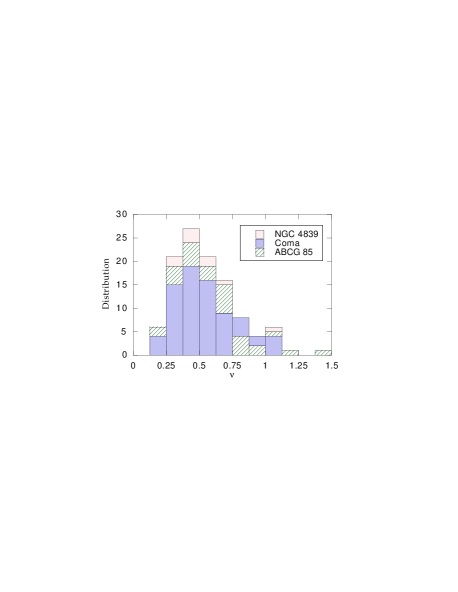
Figure 1: Distribution of the shape parameter $\nu$ for all galaxies, grouped by cluster membership. The distribution does not peak at 0.25, the value corresponding to the de Vaucouleurs profile.

Figure 2: Distribution of the intensity parameter $-2.5\log\Sigma_{0}$ (in $V$ magnitude) and the scale length $a$ (in arcsec) for all galaxies, each panel for a cluster. The bars are $1\sigma$ errors.

Figure 3: Distribution of $-2.5\log\Sigma_{0}$(in $V$ magnitude) and $\nu$. The bars are $1\sigma$ errors.

Figure 4: Distribution of $a$ (in arcsec) and $\nu$. Notice that here we have the best correlation between two of the three parameters of the Sérsic profile. The bars are $1\sigma$ errors.

Figure 5: The specific entropy relation and their corresponding residual for the elliptical galaxies in Coma, ABCG 85, and the group of NGC 4839. The straight lines are the ‘Entropic Lines’, (Eq. (29), where the slope is equal to $-1$ and the zero-points, $s_{0}$, are from Table 4: $-5.99\pm 0.20$, $-4.63\pm 0.14$, and $-4.28\pm 0.61$ for ABCG 85, Coma and NGC 4893, respectively. Note that $X(\nu)$ is a monotonic descending function of $\nu$, i.e., high values of $X(\nu)$ correspond to small $\nu$. The residual plot below each Entropic Line is $Y_{\rm data}-Y_{\rm predicted}$. The arrow in the Coma panel shows the typical displacement vector for an error in $\nu$ of 5%. This displacement is due to the definition of $X(\nu)$ and the correlations with $\Sigma_{0}$ and $a$.

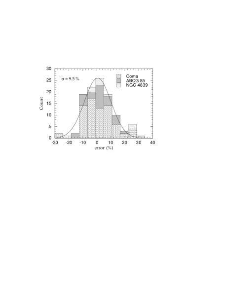
Figure 6: Dispersion distribution of the galaxies around the ‘Entropy Line’ shown in Fig. 5. This error is associated with the uncertainty in determining the specific entropy of each galaxy (see §5) and the relative distances between clusters (see §6). We show also the best fit (standard least-square method) gaussian to all data points and the one standard error, $\sigma$, in percent.

Figure 7: Scatter diagram of $\nu$ and $R_{\rm eff}$. Notice the weaker correlation in these plots compared to the correlations between the primary parameters $\nu$ and $a$.

Figure 8: Scatter diagram of $\langle\mu\rangle_{{\rm eff}}$ and $R_{\rm eff}$. The dotted lines are from the relation $\log R_{\rm eff}\propto 0.32\langle\mu\rangle_{{\rm eff}}$ found by Oegerle & Hoessel (1991) for brightest cluster members. Notice the weaker correlation in these plots compared to the correlations between the primary parameters $\Sigma_{0}$ and $a$.

The results of the growth curve fits are shown in Tables 1, 2, and 3 for Coma, ABCG 85, and the group of NGC 4839, respectively. We present also in these tables the usually quoted effective radius, $R_{\rm eff}$, and mean surface brightness $\langle\mu\rangle_{{\rm eff}}$, both computed with formulas (13) and (12), respectively. The errors in the Sérsic parameters are represented graphically in the Figures 2–4.

In Fig. 1 we show the distribution of the shape parameter $\nu$ for all our fits. The distribution is fairly regular and unimodal, but it is not symmetric (skewness $\sim 1$). It is interesting to note that $\nu=0.25$ – the value corresponding to the de Vaucouleurs profile – is neither the median ($\nu=0.50$) nor the mean ($\nu=0.55$) of the distribution. The maximum of the distribution corresponds to $\nu\sim 0.4$. Very high values of $\nu$ are obtained for a few galaxies. Although the galaxies selected by us are classified as ellipticals, our fits suggest that some of them may be in fact either lenticulars or dwarf spheroidal galaxies (those with $\nu\ga 1$). Notice, however, that our sample is not complete (we had to reject a few faint galaxies, the brightest saturated ones, and we selected only the ones with known redshift) and the distribution will be underestimated for the low surface brightness galaxies (i.e. high $\nu$).

In Figs. 2, 3, and 4 we display the relations between the primary parameters $\Sigma_{0}$, $a$, and $\nu$. It is obvious that all these quantities are strongly pairwise correlated, although non-linearly. Before analysing quantitatively these correlations, let’s make the connection with the Entropic Plane.

From Eq. (25), we expect that there are indeed non-linear correlations among the Sérsic profile parameters, since that equation defines a surface in a three dimensional space. In fact non-linear correlations are expected because the Entropic Plane relates non-linearly these parameters (if the weak or strong hypotheses hold). In order to verify whether or not Eq. (25) actually holds, we have defined two auxiliary variables:

$$Y(\Sigma_{0},a)\equiv\frac{1}{2}\ln(\Sigma_{0})+\frac{5}{2}\ln(a)\,,$$ (27)

and

$$X(\nu)\equiv c_{0}+c_{1}\ln(\nu)-\frac{1}{\nu}+c_{2}\nu^{c_{3}}\,,$$ (28)

(the constants $c_{i}$ are defined in Appendix 2). Notice that $X(\nu)$ is a monotonic descending function of $\nu$ only. With the above definitions, we can rewrite the specific entropy as a simple linear relation as:

$$Y(\Sigma_{0},a)=s_{0}-X(\nu)\,.$$ (29)

This relation defines a family of straight lines – ‘Entropic Lines’ which correspond to the Entropic Plane seen edge-on – for which the slope is $-1$ and the zero-point value (i.e. $s_{0}$, the specific entropy) is unknown.

It is straightforward to calculate $Y_{i}$ and $X_{i}$ from the values of $\Sigma_{0}$, $a$, and $\nu$ for the galaxy $i$ and, consequently, the specific entropy, $s_{0}$ for each galaxy (but notice that $s_{0}$ calculated in this way is distance dependent – we will develop this in §6). In Table 4, we give for each cluster the mean value of $s_{0}$, as well as the standard error and deviation. The zero-point of the Entropic Lines is simply the mean value of $s_{0}$ shown in Table 4.

In Fig. 5 we display $Y_{i}$ and $X_{i}$ for all our galaxies; the Entropic Line is superimposed to the data points, where we have used the values quoted in Table 4. We also show the displacement vector for a typical error in $\nu$ ($\delta\nu/\nu=0.05$); this is done taken in account the correlations of $\nu$ with both $\Sigma_{0}$ and $a$ (cf. Figs 3 and 4, as well de definition of $X(\nu)$).

Table 4: Statistic of the specific entropy. The mean value of the specific entropy, $s_{0}$, is used as the zero-point of the Entropic Line (cf. Fig. 5). While the Standard Deviation reflects the individual scatter, the Standard Error takes into account the number of data points.

	Coma	Abell85	NGC4839
Mean $s_{0}$	-4.63	-5.99	-4.28
Standard Error	0.14	0.20	0.61
Standard Deviation	1.20	1.09	1.84
Number of galaxies	73	29	9

The galaxies follow remarkably the predicted linear correlation, in spite of all our simplifying hypotheses. The small dispersion around the line representing Eq. (29) strongly suggests that in each individual cluster, these galaxies share the same specific entropy: at least the weak hypothesis is fulfilled. In Fig. 6, we show the residual distribution, i.e., $(Y_{i}-Y_{i,\rm theor})/Y_{i,\rm theor}$ (where $Y_{i}$ is obtained from the observational data and we use Eq. (29) to obtain $Y_{i,\rm theor}$ from $s_{0}-X_{i}$); the standard deviation is equal to 9.5%. Applying the Kolmogorov-Smirnov test to the residual distribution shown in Fig. 6 results that its distribution is compatible to a gaussian one. Notice, however, that due to the small number of data points, only a very deviant distribution would not be compatible with a gaussian.

It would be possible to reduce the scatter of $X_{i}$ and $Y_{i}$ by using a linear fit (slope and zero-point as free parameters) or a polynomial one instead of computing $s_{0}$ the way we did and using the predicted Entropic Line. This, however, would bury the physics behind the Entropic Plane relation – in fact, the variables $X(\nu)$ and $Y(\Sigma_{0},a)$ would lose their meaning. Anyway, fitting the $X_{i}$ and $Y_{i}$ data points to a free-slope straight line (using a standard least-square method) yields the following slopes: $-0.84\pm 0.05$, $-0.93\pm 0.06$, and $-0.66\pm 0.12$ for Coma, Abell 85, and NGC 4839 group, respectively. The mean value of the slope, taking into account the error bars, is $0.86\pm 0.14$. Although this is statistically consistent with the predicted Entropic Line, the tilt is almost certainly real. There is a number of effects that may account for the scatter and the deviation of the data points from a line of slope exactly equal to $-1$. This point will be addressed in §7.

Table 5: Non parametric correlation tests between the parameters of the Sérsic-law for the Coma cluster. Both $\rho$ and $\tau$ are defined in the interval $[-1,1]$, the value 0 meaning no correlation. Higher absolute values of $z$ indicate a greater significance of the correlations.

Parameters	$|\rho|$ Spearman	$|z|$	$|\tau|$ Kendall	$|z|$
$X(\nu)$–$Y(\Sigma_{0},a)$	0.94	7.97	0.82	10.3
$\nu$–$a$	0.95	8.10	0.84	10.5
$\nu$–$\Sigma_{0}$	0.89	7.57	0.73	9.18
$a$–$\Sigma_{0}$	0.89	7.56	0.73	9.18
$\nu$–$R_{{\rm eff}}$	0.51	4.36	0.37	4.65
$R_{{\rm eff}}$–$\langle\mu\rangle_{{\rm eff}}$	0.18	1.54	0.13	1.60

Table 6: Same as Table 5 for ABCG 85.

Parameters	$|\rho|$ Spearman	$|z|$	$|\tau|$ Kendall	$|z|$
$X(\nu)$–$Y(\Sigma_{0},a)$	0.95	5.03	0.84	6.38
$\nu$–$a$	0.97	5.13	0.88	6.68
$\nu$–$\Sigma_{0}$	0.89	4.71	0.80	6.04
$a$–$\Sigma_{0}$	0.85	4.52	0.74	5.63
$\nu$–$R_{{\rm eff}}$	0.32	1.67	0.22	1.65
$R_{{\rm eff}}$–$\langle\mu\rangle_{{\rm eff}}$	0.31	1.64	0.21	1.61

Table 7: Same as Table 5 for NGC 4839 group.

Parameters	$|\rho|$ Spearman	$|z|$	$|\tau|$ Kendall	$|z|$
$X(\nu)$–$Y(\Sigma_{0},a)$	0.97	2.73	0.89	3.34
$\nu$–$a$	0.97	2.73	0.89	3.34
$\nu$–$\Sigma_{0}$	0.92	2.59	0.78	2.92
$a$–$\Sigma_{0}$	0.92	2.59	0.78	2.92
$\nu$–$R_{{\rm eff}}$	0.42	1.18	0.33	1.25
$R_{{\rm eff}}$–$\langle\mu\rangle_{{\rm eff}}$	0.20	0.56	0.06	0.21

Similar to our Fig. 4, Young & Currie (1995) have already presented the $\nu$–$a$ correlation for dwarf ellipticals in the direction of the Fornax cluster (figure 1 in their paper) and fitted it with a polynomial having five free parameters. Their small r.m.s. scatter (0.108) suggested that the $\nu$–$a$ correlation could be a useful distance indicator. More recently, Binggeli & Jerjen (1998), who have also fitted the growth curve using the Sérsic profile, have presented the same correlation between the shape parameter and the scale length for early-type galaxies belonging to the Virgo cluster (Fig. 7 in their paper). They have fitted a parabola to the $\nu$–$a$ correlation and have derived a r.m.s. equal to 17%.

We have mentioned in Section 3.1 that the ‘astrophysical’ parameters are non-linear combinations of the primary parameters. It is therefore not surprising that the correlations between these quantities are less clear compared to the corresponding relations obtained when one uses the primary parameters. For instance, the distribution of $R_{\rm eff}$ and $\nu$ (Fig. 7) compared to the distribution of $a$ and $\nu$ (Fig. 4) shows how the primary parameters correlates better than the classical astrophysical parameters. One can also see the Fig. 3 from the paper by Graham et al. (1996), where they plot the $R_{\rm eff}$–$\nu$ relation and compare it with the $a$–$\nu$ relation displayed in Fig. 7 from the paper of Binggeli & Jerjen (1998) for Virgo galaxies. Finally, one can compare the computed values of $R_{\rm eff}$ and $\langle\mu\rangle_{{\rm eff}}$ (Fig. 8) and compare it to the relation between $-2.5\log\Sigma_{0}$ and $a$ (Fig. 3).

As already noted by Oegerle & Hoessel (1991), the scatter is rather larger for normal elliptical galaxies than for the brightest cluster members (BCG). In Fig. 8 we have superposed the empirical relation $\log R_{\rm eff}\propto 0.32\langle\mu\rangle_{{\rm eff}}$ found by Oegerle & Hoessel (1991, their Fig. 5) for their sample of BCGs. It is clear from Fig. 8 that this is the most scattered relation.

The relations observed in Figs. 2, 3, and 4 are nothing more than projections of the Entropic Plane predicted by Eq. (25) onto the three planes defined by the parameters $\Sigma_{0}$, $a$, and $\nu$. The thickness of the pairwise correlations seen in these figures is largely due to the fact that the specific Entropic Plane is not seen exactly edge-on. The non-linear combinations of these parameters (the $R_{\rm eff}$–$\langle\mu\rangle_{\rm eff}$ correlation, for instance) present, as one would expect, greater scatter. By the same token, one could naïvely expect that the scatter of the $X_{i}$–$Y_{i}$ relation (which is also a non-linear combination of the Sérsic parameters) would be greater than the scatter of the primary parameters pairwise correlations.

In Tables 5 to 7, we quantify the quality of the Sérsic parameters pairwise relations using two non-parametric analysis: the Spearman and the Kendall rank correlation tests (for a detailed description, see Siegel & Castellan 1989; Press et al. 1992). (In §6 below, we will give the scatter around the Entropic Line in terms of the distance modulus for each galaxy in Fig. 9.) As it can be seen, the relations involving the secondary parameters, $R_{\rm eff}$ and $\langle\mu\rangle_{\rm eff}$, have indeed smaller correlation coefficients than the relations involving only the primary Sérsic parameters.

The Entropic Line turns out to have about the same correlation coefficients as the $\nu$–$a$ relation (the latter being slightly more tightly correlated). This tells us that the Entropic Line does not seem to be just an arbitrary non-linear combination of the primary parameters, but may be indeed a fundamental relation based on the assumption of unique specific entropy. It also tells us that the $\nu$–$a$ relation is almost an edge-on projection of the Entropic Plane. The fact that the Entropic Line has not a better correlation coefficient may be due to one or some of our simplifying hypotheses in deriving the specific entropy relation for elliptical galaxies (for instance, the ideal gas, the isotropic pressure, and the mass–luminosity ratio, see also §7).

6 Towards a distance indicator

6.1 Distance dependence

The specific entropy can be written as a function of the three parameters of the Sérsic profile (cf. Eq. 25). If we could somehow determine the value of the specific entropy for a given galaxy, then we would have a relation linking one of the parameters as a function of the remaining two others, for instance, $\nu(a,\Sigma_{0})$.

Any relation that operates between a dimensionless parameter and one or more distance-dependent parameters can be potentially used as a distance indicator. In the present case, a correlation between the distance independent $\nu$ and the distance dependent $a$ and $\Sigma_{0}$ could be used as a yardstick.

However, a difficulty arises since we need to know a priori the value of the specific entropy. This problem can be solved partially if we consider relative distances between clusters of galaxies (but not individual galaxies) instead of absolute distances. Measuring the distances of clusters instead of individual galaxies reduces the error induced by the dispersion in the specific entropy relation.

The parameters $a$ and $\Sigma_{0}$ are, so far, given in metric units, not angular. The distance dependence of $Y$, defined in Eq. (27), can be written explicitly by converting $a$ and $\Sigma_{0}$ to those observed, $a\hbox{${}^{\prime\prime}$}$ and $\Sigma_{0}\hbox{${}^{\prime\prime}$}$, as follows:

$$Y=\frac{1}{2}\ln(\Sigma_{0}\hbox{${}^{\prime\prime}$})+\frac{5}{2}\ln(a\hbox{${}^{\prime\prime}$})+\frac{3}{2}\ln(D)\,$$ (30)

where $D$ is the distance to the cluster.

The fits of the growth curves provide us with the parameters $\Sigma_{0}\hbox{${}^{\prime\prime}$}$, $a\hbox{${}^{\prime\prime}$}$, and $\nu$, thus the parameters $X$ and $Y$ (without the distance term). Given a sample of early type galaxies from a cluster of known distance, we obtain the specific entropy as the mean value of $s_{0}$ found for all sample galaxies in that cluster, provided that Hypothesis I holds.

6.2 Relative distances

Likewise, given two samples of galaxies on two different clusters of unknown distances, and assuming that Hypothesis II holds, we could determine the relative distance of the clusters directly from Eq. (30). The relative distance between two clusters is given by

$$\frac{D_{1}}{D_{2}}=\exp\left(\frac{s_{2}-s_{1}}{1.5}\right)\,,$$ (31)

where $s_{i}$’s are the mean entropy of each cluster. To these distance corresponds the relative distance modulus, $\mu$:

$$\mu_{1}-\mu_{2}=-1.448(s_{1}-s_{2})$$ (32)

Applying Eq. (32) to Coma, ABCG 85, and the group of NGC 4839, we obtain:

$$\mu_{\rm ABCG85}-\mu_{\rm Coma} = 1.98\pm 0.33$$

$$\mu_{\rm NGC4839}-\mu_{\rm Coma} = -0.51\pm 0.53\,$$ (33)

The mean entropy are taken from Table 4 while errors are deduced from the standard error propagation.

In term of relative distances we have:

$$D_{\rm ABCG85}/D_{\rm Coma} = 2.5^{+0.4}_{-0.3}$$

$$D_{\rm NGC4839}/D_{\rm Coma} = 0.8^{+0.2}_{-0.5}\,$$ (34)

The error bars seems especially large in the case of NGC 4839/Coma distance. Notice however that the number of galaxies used in this case is very low (9 galaxies in the group of NGC 4839); the error bars would be $\sim 0.2$ if we had a sample of about a hundred galaxies in the group.

For comparison, the relative distance between ABCG 85 and Coma derived from their mean redshifts is $\sim 2.4$, cf. Biviano et al. (1995b), Durret et al. (1998). If we suppose that the distance of ABCG 85 is given by (34) so that its redshift is a composition of Hubble velocity plus its peculiar velocity, and a contrario that Coma is at rest in its Hubble frame, then ABCG 85 would have a line of sight peculiar velocity of $\sim-600\pm 240$km s^-1.

It seems that this method is not adequate to determine individual distances inside a cluster. In Fig. 9 we show for each cluster the distribution of the distance modulus, $\mu$, computed for each galaxy using the Eq. (31) relative to the mean specific entropy (the values in Table 4). The r.m.s. scatter is about 1.1 mag for the rich clusters. Nonetheless, we note that using only the $a-\nu$ correlation, following Young & Currie (1995) or Binggeli & Jerjen (1998), and fitting it with an arbitrary polynomial of either 3 or 5 free parameters, we obtain scatters of the order of 0.83 mag.

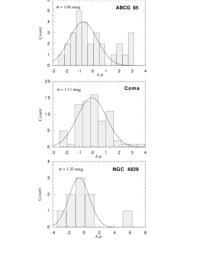
Figure 9: Distribution of the distance modulus, $\mu$, for each cluster computed using Eq. (31). The superposed curves are gaussian fits (using a standard least square method) and in each panel is quoted the standard error in magnitude. Notice that scales are different in each panel.

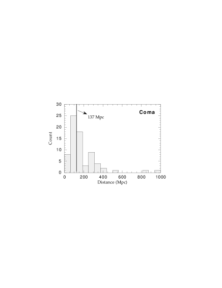
Figure 10: Individual distances of the galaxies in Coma computed using Eq. (31) and assuming the centre of the cluster is at 137 $h^{-1}_{50}$ Mpc. Notice how this artificially stretches the cluster in the line-of-sight direction.

For the Coma cluster we also show the dispersion in relative distances (Fig. 10), assuming that the centre of Coma is at 137 $h^{-1}_{50}$ Mpc (Colless & Dunn 1996; Durret et al. 1998).

The scatter around the Entropic Plane is not produced by the distances of individual galaxies with respect to the centre of mass, but it is due to a number of effects that will be discussed in the next section. This scatter produces an artificially elongated cluster; in the present case of Coma, we obtain a depth of $\sim 1000$ Mpc or, neglecting the 5 most ‘distant’ galaxies, a depth of $\sim 350$ Mpc.

7 Discussion

From previous work (Young & Currie 1994, 1995; Binggeli & Jerjen 1998) and from our own data of elliptical galaxies in two rich clusters and a group, it is clear that there are strong correlations among the primary free parameters of the Sérsic profile. Before exploring the possible application of this relationship, we tried to understand the physics underlying it.

Since isolated elliptical galaxies seem to be systems in quasi-equilibrium, i.e., only subject to secular evolution, we assume that their dynamical state is characterised by a stationary entropy. We can go further and postulate that the entropy per mass unit (specific entropy, $s$) would be the same for all galaxies. In order to confront this hypothesis against observational data, we needed to compute this specific entropy. From Sérsic’s light (and mass) distribution for elliptical galaxies, and assuming the equations of state of an ideal gas, as well as the isotropy of the velocity tensor, we have derived a theoretical relationship among the parameters describing Sérsic’s profile. This relation defines an ‘Entropic Plane’.

We have found that these primary parameters for a given cluster or group are well approximated by the predicted constant specific entropy relation: elliptical galaxies seem to share the same $s$.

We would like to emphasise that the two principal assumptions that we have used, i.e., the entropy and the ideal gas equations of state, are not straightforward concepts in the context of stellar self-gravitating dynamics. Interestingly, these supposedly inefficient tools allow us to predict relations which match quite well the observational data, a result which raises interesting questions on the description of self-gravitating systems.

Nevertheless, we note that the observations are quite dispersed along the Entropy Line given by Eq. (29) and that there appears to be a tilt between de data and the predicted Entropy Line (Fig. 5). A number of effects could account for this result.

• Concerning the model:

  • we have used a constant $M/L$ ratio. This is the simplest way to account for the relative contribution of different light components in a galaxy, and for ellipticals as a whole, given our knowledge of the $M/L$ trend in these galaxies (Jørgensen 1997). Notice that the specific entropy varies as $\ln(M/L)$. Such a weak dependence on $M/L$ (which we suppose constant from one galaxy to another), may certainly explain why the predicted correlations work so well even if, indeed, there is a variation of $M/L$ as a function of $\nu$ (and consequently of the total mass of the galaxy);

  • for the hydrostatic equilibrium we have considered the velocity dispersion tensor to be isotropic. This is probably correct for galactic centres, but it is probably not for the outskirts. At present, only the introduction of a phenomenological parameter describing the variation of the anisotropy with galactocentric distance would account for such a dispersion;

  • the equations of state that we have used are for ideal, non-interacting, hot gas. The inclusion of self-gravity explicitly (it is implicitly included by way of the hydrostatic equilibrium and Poisson equations) will probably tilt the Entropic Plane since the total mass of the galaxy correlates with the Sérsic parameter, in particular $\nu$;

  • galaxies are likely to undergo merging and/or collisions, especially in clusters; therefore during these events they will necessarily escape from the ‘Entropic Plane’. However, the resulting galaxies are expected to return back to the ‘Entropic Plane’ after a given relaxation time.

• Concerning the data analysis:

  • In Fig. (1) we have given the distribution of $\nu$; we note that this distribution is different from that of Virgo galaxies given by Graham & Colless (1997). On the other hand, our distribution of $\nu$ is similar to the one obtained by Binggeli & Jerjen (1998). This seems to indicate that, in order to obtain comparable results, it is very important to use the same procedure to analyse the data.

As noted in the previous section, galaxies in a cluster are not exactly at the same distance from us, and the scatter around the ‘Entropy line’ is partly due to the various (physical and observational) effects noted above. The scatter is thus larger than that due only to distance variations. We have used Formula (31) for each galaxy in the Coma cluster compared to the mean $s$ (the zero-point for the cluster). The Coma cluster then appears extremely elongated along the line-of-sight; Binggeli & Jerjen (1998) conclude in the same vein when discussing the application of the profile based distance indicator to individual galaxies in the Virgo cluster made by Young & Currie (1995) [but see also Young & Currie (1998), who refute the analysis of Binggeli & Jerjen].

The ‘Entropic Plane’ appears to be essentially useful to determine the distance to clusters, but not to individual galaxies inside a cluster, at least with the present scatter; notice that it is also the case for the Tully-Fisher relation, which is used to compare relative distances between clusters (Scodeggio et al. 1997).

8 Conclusion

The distance indicator we propose is not new, in the sense of using the distance independent shape parameter $\nu$ (or a function depending only of $\nu$) of the Sérsic law as a yardstick (cf. Young & Currie 1994, 1995, who proposed a distance indicator based on the shape profile of elliptical galaxies and applied it to the Fornax and Virgo clusters). Our distance indicator, however, was derived from thermodynamics equilibrium, based on our strong hypothesis: i.e. the specific entropy of relaxed galaxies is universal. As noted in the introduction, this should be a natural consequence of some violent relaxation process; the universality, however, seems not to be guaranteed since the history or evolutionary stage of a given cluster may have some influence in the formation process of galaxies and consequently may produce some variations in the resulting specific entropy.

Therefore, seeking a physical explanation for the profile-shape distance indicators allowed us to derive a variant distance indicator that has only one free parameter, namely the specific entropy of galaxies. That should be compared with the empirical profile-shape distance indicators [Young & Currie 1994, 1995; Binggeli & Jerjen (1998)] that need 3 to 5 free parameters. Nevertheless, since the exact shape of the Entropic Plane depends on the way we model the elliptical galaxies, the empirical profile-shape distance indicators have a smaller intrinsic scatter.

Concerning the unique specific entropy of elliptical galaxies being independent of the cluster in which they are located, if the existence of an universal profile (Navarro et al. 1995) is confirmed, the peculiar properties of clusters should not be very important. In this case, the relation expressed by Eq. (29) may provide some clue to the relaxation process in galaxies in addition to an attractive way to measure relative distances between clusters, using only photometrical data – in contrast to the Fundamental Plane which requires spectroscopic data as well.

9 Acknowledgments

We are very grateful to J.M. Alimi, H.V. Capelato and H. Verhagen for helpful comments and discussions. We wish to thank F. Durret for making available the ABCG 85 data to us and for helpful comments. We thank C. Lobo for helping us with the Coma catalogue. This paper is based on observations collected at the Canada-France-Hawaii telescope (operated by the National Research Council of Canada, the Centre National de la Recherche Scientifique of France, and the University of Hawaii) and the European Southern Observatory, La Silla, Chile.

Appendix 1

In Section 2.1 we derive the specific entropy from the fundamental relation of thermodynamics. Here, show that an equivalent form is obtained using the Boltzmann-Gibbs entropy:

$$s=-\frac{S}{M}\int_{\Omega}F\ln(F){\rm d}^{3}x{\rm d}^{3}v\,,$$ (35)

where $\Omega$ is the volume in phase space and $F$ is the distribution function. From the definition of a mean value, Eq. (35) can be re-written as:

$$s=\left\langle{\ln({F}^{-1})}\right\rangle\,.$$ (36)

The distribution function can also be interpreted as the mass density in phase space, ${\rm d}M/({\rm d}^{3}x{\rm d}^{3}v)$. Thus it is legitimate to express $F$ as:

$$F\propto\rho/\sigma^{3}\,,$$ (37)

where $\sigma$ is the velocity dispersion and $\rho$ the density. Now, we need an equation of state. Adopting the following form:

$$P=K\rho^{\gamma}\sigma^{2}\,,$$ (38)

(a polytrope of index $n=1/(\gamma-1)$ [Binney & Tremaine 1987, p. 224]) and substituting it in Eq. (37) and (36) we finally get:

$$s=\left\langle{\ln\left(\rho^{-(1+3\gamma/2)}P^{3/2}\right)}\right\rangle\,.$$ (39)

For $\gamma=1$ (ideal gas) we recover Eq. (6).

Appendix 2

The numerical computation of Eq. (6) for an arbitrary choice of $\nu$, $a$ and $\Sigma_{0}$ is cumbersome and slow. Here, we will derive a simple analytical approximation for the specific entropy for a galaxy following the Sérsic law. We do this in two steps.

(I) First we look for a simple functional form that describes $s$ as a function of the Sérsic parameters.

In section 2.1 we show that the specific entropy can be expressed as a mean value, cf. Eq. (6). We rewrite it as:

$$s\approx-\frac{5}{2}\ln(\rho_{\rm eff})+\frac{3}{2}\ln(P_{\rm eff})+C\,,$$ (40)

where we have used the approximation $\langle x\rangle\propto x_{\rm eff}$, with $x_{\rm eff}$ meaning the value of $x(r)$ taken at $r=R_{\rm eff}$, the effective radius, and $C$ is a constant of proportionality. Although this approximation is justified for homologous, isotropic systems, it is in principle not so for the Sérsic profile. Our goal here, however, is just to obtain a rough analytical form that will later be fine tuned.

Both $\rho_{\rm eff}$ and $P_{\rm eff}$ can be computed numerically from Eqs. (13), (17) and(24). For the effective density, we have to a good approximation the following analytical expression:

$$-\frac{5}{2}\ln(\rho_{\rm eff})\approx-\frac{5}{2}\ln(\rho_{0})+4.75\nu^{-1.46}\,,$$ (41)

and, for the effective pressure we have:

$$\frac{3}{2}\ln(P_{\rm eff})\approx\frac{3}{2}\ln(4\pi\;G)+3\ln\left(\frac{a\;\rho_{0}}{\nu}\right)-4.1\nu^{-1.0}\,.$$ (42)

Both formulae are analytical fits that give the dependence of $\rho_{\rm eff}$ and $P_{\rm eff}$ on the parameters of the Sérsic profile.

We also need the relation between the three dimensional central mass density, $\rho_{0}$, and the projected central light density, $\Sigma_{0}$. This can be fairly well approximated as:

$$\rho_{0}\approx\frac{\Sigma_{0}}{a}\;\frac{M}{L}\;0.36\nu^{0.60}\,.$$ (43)

Substituting Eqs. (41), (42), and (43) into Eq. (40), we obtain an analytical expression:

$$s \approx \frac{1}{2}\ln(\Sigma_{0})+\frac{5}{2}\ln(a)+\frac{1}{2}\ln\left(\frac{M}{L}\right)+\frac{3}{2}\ln(G)$$ (44)

$$+ c_{0}+c_{1}\ln(\nu)-\frac{1}{\nu}+c_{2}\nu^{c_{3}}\,,$$

where the constants $c_{i}$ are to be determined and fine-tuned.

(II) The second step is to use the above formula as a template to obtain an accurate approximation independent of $R_{\rm eff}$.

This is done by fitting the analytical approximation, Eq. (44), to the formula of the specific entropy, Eq. (6) (which can be computed numerically). We then get the following values for the constants $c_{i}$:

$$c_{0}=-0.299,\quad c_{1}=-0.058,\quad c_{2}=3.656,\quad c_{3}=-1.327\,.$$

The fit is done using a standard least-square method, computing Eq. (6) in a ‘cube’ with the axes $\nu$, $a$ and $\Sigma_{0}$. Taking the $M/L$ ratio as independent of the galactic radius as well as constant for all galaxies and scaling $G$ appropriately, we obtain the entropy relation expressed in Eq. (25), using the above numerical values for the $c_{i}$’s (the numerical value of $c_{0}$ has the term $(3/2)\ln G$ folded in).

The analytical approximation is accurate to better than 2% in the range $0.15\leq\nu\leq 1.85$ and the ratios $a_{\rm max}/a_{\rm min}=1.2\times 10^{4}$ and ${\Sigma_{0}}_{\rm max}/{\Sigma_{0}}_{\rm min}=2.3\times 10^{7}$ (for $a$ and $\Sigma_{0}$ only the ratio is relevant since the values can be scaled with the choice of units of $G$). Considering that the $M/L$ ratio varies at most as $M^{0.2}$ (Pahre et al. 1995) and that the range in galaxy masses we are interested in is less than $10^{4}$, then the $M/L$ ratio varies at most by a factor $\sim 6$.

Although the functional dependence of the Sérsic parameters in Eq. (44) was found with the help of the rough approximations given by Eqs. (41) and (42), the $\Sigma_{0}$ and $a$ dependencies are the same as in the case of a sphere obeying the Plummer density profile (where we can calculate exactly the specific entropy).

References

- [1] Antonov V.A., 1962, Vest. Leningrad Univ. 7, 135 (Translated in: IAU Symp. 113 ‘Dynamics of star clusters’, 1985, p.525, Goodman J., Hut P. eds., Reidel:Dordrecht)
- [Bender & Möllenhoff 1987] Bender R., Möllenhoff C., 1987, A&A 177, 71
- [2] Bender R., Burstein D., Faber S., 1992, ApJ 399, 462
- [3] Bertin G., Bertola F., Buson L.M., Danziger I.J., Dejonghe H., Sadler E.M., Saglia R.P., de Zeeuw P.T., Zeilinger W.W., 1994, A&A 292, 381
- [4] Binggeli B., Jerjen H., 1998, A&A 333, 17
- [5] Binney J., 1982, MNRAS 200, 951
- [6] Binney J., Tremaine S., 1987, ‘Galactic Dynamics’, Princeton Series in Astrophysics, Princeton, New Jersey
- [Biviano et al. 1995] Biviano A., Durret F., Gerbal D., Le Fèvre O., Lobo C., Mazure A., Slezak E., 1995a, A&A Suppl. 111, 265
- [Biviano et al. 1995] Biviano A., Durret F., Gerbal D., Le Fèvre O., Lobo C., Mazure A., Slezak E., 1995b, A&A 297, 610
- [7] Bonnor W.B., 1956, MNRAS 116, 351
- [8] Burstein D., Davies R.L., Dressler A., Faber S.M., Stone R.P.S., Lynden-Bell D., Terlevich R.J., Wegner G., 1987, ApJ Suppl. 64, 601
- [9] Callen H.B., 1960, ‘Thermodynamics’, John Wiley & Sons, Inc, New York
- [Caon et al. 1993] Caon N., Capaccioli M., D’Onofrio M., 1993, MNRAS 265, 1013
- [10] Carollo C.M., de Zeeuw P.T., van der Marel R.P., Danziger I.J., Qian E.E., ApJ 441, L28
- [Ciotti 1991] Ciotti L., 1991, A&A 249, 99
- [11] Ciotti L., Lanzoni B., 1997, A&A 321, 724
- [Colless & Dunn 1996] Colless M., Dunn A. M., 1996, ApJ 458, 435
- [Courteau et al. 1996] Courteau S., de Jong R. S., Broeils A. H., 1996, ApJ 457, L73
- [12] Dejonghe H. 1987, ApJ 320, 477
- [de Vaucouleurs 1948] de Vaucouleurs G., 1948, Ann. Astrophys. 11, 247
- [13] de Zeeuw P.T., Franx M., 1991, ARA&A 29, 239
- [14] de Zeeuw P.T., 1992, in: ‘Morphological and Physical Classification of Galaxies’, p. 139, Kluwer Acad. Publ., Longo G., Capaccioli M., Busarello G. (eds.)
- [Djorgovski & Davies 1987] Djorgovski S., Davis M., 1987, ApJ 313, 59
- [15] D’Onofrio M., Prugniel Ph., 1997, in:‘Dark and Visible Matter in Galaxies’, ASPCS 117, p. 568, Persic M., Salucci P. eds.
- [Dressler et al. 1987] Dressler A., Faber S.M., Burstein D., Davies R.L., Lynden-Bell D., Terlevich R.J., Wegner G. 1987a, ApJ 313, L37
- [Dressler et al. 1987] Dressler A., Lynden-Bell D., Burstein D., Davies R.L., Faber S.M., Terlevich R.J., Wegner G., 1987b, ApJ 313, 42
- [16] Durret F., Felenbok P., Lobo C., Slezak E., 1998, A&A Suppl. 129, 281
- [Gerbal et al. 1997] Gerbal, D., Lima Neto, G.B., Márquez, I., Verhagen, H., 1997, MNRAS 285, L41
- [17] Godwin J., Metcalfe N., Peach J.V., 1983, MNRAS 202, 113
- [Graham et al. 1996] Graham A., Lauer T.R., Colless M., Postman, M., 1996, ApJ 465, 534
- [Graham & Colless. 1997] Graham A., Colless M., 1997, MNRAS 287, 221
- [18] Hjorth J., Madsen J., 1995, ApJ 445, 55
- [19] Jørgensen I., 1997, MNRAS 288, 161
- [Kormendy 1977] Kormendy J., 1977, ApJ 218, 333
- [Kormendy 1984] Kormendy J., 1984, ApJ 287, 577
- [Lobo et al. 1997] Lobo C., Biviano A., Durret F., Gerbal D., Le Fèvre O., Mazure A., Slezak E., 1997, A&A Suppl. 122, 409
- [Lynden-Bell 1967] Lynden-Bell D., 1967, MNRAS 136, 101
- [Lynden-Bell & Wood 1968] Lynden-Bell D., Wood R., 1968, MNRAS 138, 495
- [Mellier & Mathez 1987] Mellier Y., Mathez G., 1987, A&A 175, 1
- [20] Merritt D., Tremaine S., Johnstone D., 1989, MNRAS 236, 829
- [Michard 1985] Michard R., 1985, A&A Suppl. 59, 205
- [21] Navarro J.F., Frenk C.S., White S.D.M., 1995, MNRAS 275, 720
- [Oegerle & Hoessel 1991] Oegerle W.R., Hoessel J.G., 1991, ApJ 375, 15
- [22] Pahre M.A., Djorgovski S.G., de Carvalho R.R., 1995, ApJ 453, L17
- [Petrosian 1976] Petrosian V., 1976, ApJ 209, L1
- [23] Press W.H., Teukolsky S.A., Vetterling W.T., Flannery B.P., 1992, ‘Numerical Recipes in Fortran’, 2nd ed. Cambridge University Press
- [Prugniel & Simien1997] Prugniel Ph., Simien F., 1997, A&A 321, 111
- [24] Richstone D.O., Tremaine S., 1988, ApJ 327, 82
- [25] Rix H.W., de Zeeuw P.T., Cretton N., van der Marel R., Carollo C.M., 1997, ApJ 488, 702
- [Sandage & Perelmuter 1990] Sandage A., Perelmuter J.-M., 1990, ApJ 350, 481
- [26] Saslaw W.C., 1985, ‘Gravitational Physics of Stellar and Galactic Systems’, Cambridge Univ. Press
- [Schombert 1986] Schombert J.M., 1986, ApJ Suppl. 60, 603
- [Schombert 1988] Schombert J.M., 1988, ApJ 328, 475
- [Sérsic 1968] Sérsic J.L., 1968, Atlas de galaxias australes, Observatorio Astronómico de Córdoba, Argentina
- [27] Scodeggio M., Giovanelli R., Haynes M.P., 1997, AJ 113, 2087
- [28] Shu F.H., 1978, ApJ 225, 83
- [29] Siegel S., Castellan N.J., Jr, 1989, ‘Nonparametric Statistics for Behavioral Sciences’, 2nd ed. McGraw-Hill, New York
- [30] Slezak E., Durret F., Guibert J., Lobo C., 1998, A&A Suppl. 128, 67
- [31] Spergel D.N., Hernquist L., 1992, ApJ Lett. 397, L75
- [32] Stiavelli M., 1998, ApJ Lett. 495, L91
- [33] Tremaine S., Hénon M., Lynden-Bell D., 1986, MNRAS 219, 285
- [34] Tully R.B., Fisher J.R., 1977, A&A 55, 661
- [White & Narayan 1987] White S.D.M., Narayan, R., 1987, MNRAS 229, 103
- [35] Young P.J., 1976, AJ 81, 807
- [Young & Currie 1994] Young C. K., Currie M. J., 1994, MNRAS 268, L11
- [Young & Currie 1995] Young C. K., Currie M. J., 1995, MNRAS 273, 1141
- [36] Young C. K., Currie M. J., 1998, A&A 333, 795