Power Density Spectra of Gamma-Ray Bursts in the Internal Shock Model

Abstract

We simulate Gamma-Ray Bursts arising from internal shocks in relativistic winds, calculate their power density spectrum (PDS), and identify the factors to which the PDS is most sensitive: the wind ejection features, which determine the wind dynamics and its optical thickness, and the energy release parameters, which give the pulse 50–300 keV radiative efficiency. For certain combinations of ejection features and wind parameters the resulting PDS exhibits the features observed in real bursts. We found that the upper limit on the efficiency of conversion of wind kinetic energy into 50–300 keV photons is $\sim$ 1%. Winds with a modulated Lorentz factor distribution of the ejecta yield PDSs in accord with current observations and have efficiencies closer to $10^{-3}$, while winds with a random, uniform Lorentz factor ejection must be optically thick to the short duration pulses to produce correct PDSs, and have an overall efficiency around $10^{-4}$.

Department of Astronomy & Astrophysics, Pennsylvania State University, University Park, PA 16802

Subject headings: gamma-rays: bursts - methods: numerical - radiation mechanisms: nonthermal

1 Introduction

Internal shocks occurring in a transient, unstable relativistic wind (Rees & Mészáros 1994) are believed to be the source of the $\sim 100$ keV emission and the complex temporal structure of Gamma-Ray Bursts (GRBs). The shocks resulting from such instabilities heat the expanding ejecta, amplify pre-existing magnetic fields or generate a turbulent one, and accelerate electrons, leading to synchrotron emission and inverse Compton scatterings. Synchrotron self absorption and pair formation may further shape the emergent spectrum, depending on the choice of model parameters, as shown by Papathanassiou & Mészáros (1996) and Pilla & Loeb (1998). The spectrum of the emitted radiation has also been analyzed by Daigne & Mochkovitch (1998) and Panaitescu & Mészáros (1999). The synchrotron self-Comptonized emission from internal shock GRBs has also been studied by Sari & Piran (1997) and Ghisellini & Celotti (1999).

In this paper we analyze the temporal features of GRBs obtained in the framework of relativistic winds, through the burst power density spectrum (PDS). The recent work of Beloborodov, Stern & Svensson (1998) has put into evidence interesting PDS features, which we use for analyzing some of the model parameters and the features of the wind ejection. We use the observed integral burst intensity ($\log N-\log P$) distribution (Pendleton et al. 1996) as a constraint in our choice for some of the model parameters. Other properties of the observed light curves, such as the distribution of pulse durations (Norris et al. 1996) or those of pulse fluences and time intervals between peaks (Li & Fenimore 1996), can also be used in the study of the wind ejection features (Spada, Panaitescu & Mészáros 1999).

2 Outline of the Model Features

The model used here is similar to that developed by Daigne & Mochkovitch (1998), and is different in the following ways. Our treatment of the radiation emission takes into account the up-scattering of the synchrotron photons, which may be the dominant emission process at $\sim 100$ keV if the magnetic field is sufficiently low. The optical thickness (to Thomson scatterings) of the wind is taken into account, which may be very important for the burst PDS and overall efficiency. We use the shock jump equations to determine the physical conditions in the shocked fluid and we include the effects arising from electron cooling in the shape of the emission spectrum.

After setting the dynamics of the wind ejection, we calculate the radii where internal collisions take place, determine the relevant physical parameters in the shock fluid – bulk Lorentz factor (LF), typical electron random, magnetic field, etc. – and calculate the features of the emitted radiation: energy of the synchrotron and inverse Compton spectral peaks (with allowance for the Klein-Nishina effect), Comptonization parameter, 50–300 keV emission (accounting for scattering during propagation through the wind), and its duration. These quantities are necessary for the computation of the observer frame pulse features: fluence, duration, arrival time, taking into account relativistic and cosmological effects. Assuming the two-sided exponential pulse shape identified by Norris et al. (1996) in real bursts, one can calculate the peak photon flux for each pulse. Below we describe the most important aspects related to the calculation of the some of the above mentioned quantities.

The wind is discretized as a sequence of shells, released by the central source during a time $t_{w}$ and with an average interval $t_{v}$ between consecutive ejections, so the number of shells is just $N=t_{w}/t_{v}$. The mass of each shell is drawn from a log-normal distribution determined by the average shell mass $\overline{M}=M_{w}/N$, $M_{w}$ being the wind mass, and a dispersion $\sigma_{M}=\overline{M}$. The LF $\eta$ of each shell is randomly drawn from the interval $[\eta_{m},\eta_{M}]$. Both $\eta_{m}$ and $\eta_{M}$ can be chosen constant during the entire wind ejection, so that $\eta$ has a uniform distribution (we shall refer to this case as the ”uniform wind”), or can vary on time-scale comparable to $t_{w}$ and much larger than $t_{v}$, according to a certain law. For brevity, in the latter case, we shall keep $\eta_{m}$ constant and use an $\eta_{M}$ that varies with ejection time as a square sine with only one oscillation (this will be the ”modulated wind”), thus the LF of the $j^{\rm th}$ ejected shell is

$$\eta_{j}=\eta_{m}+a_{j}\sin^{2}(\pi j/N)(\eta_{M}-\eta_{m})\quad 1\leq j\leq N\;,$$ (1)

where $a_{j}$ is a random number between 0 and 1. The time elapsed before the ejection of a shell is chosen to be proportional to the energy of that shell, thus leading to a wind luminosity $L_{w}$ that is constant on average throughout the entire wind ejection.

The shock-accelerated electrons have a power-law distribution of index $-p$, starting from a low random LF set by the electron injection fraction $\zeta\mathrel{\hbox to0.0pt{\raise 2.20013pt\hbox{$<$}\hss}{\lower 2.20013pt\hbox{$\sim$}}}1$ and the fraction $\varepsilon_{e}$ of the internal energy stored in the electrons:

$$\gamma_{m}=\frac{p-2}{p-1}\frac{\varepsilon_{e}u^{\prime}}{\zeta n^{\prime}_{e}m_{e}c^{2}}\stackrel{{\scriptstyle\epsilon_{dis}\ll 1}}{{=}}1837\frac{p-2}{p-1}\frac{\varepsilon_{e}}{\zeta}\epsilon_{dis}\;,$$ (2)

where $u^{\prime}$ and $n^{\prime}_{e}$ are the comoving frame internal energy density and electron number density of the shocked fluid, respectively, which we calculate with the aid of the shock jump conditions, and $\epsilon_{dis}$ is the dissipation efficiency, i.e. the fraction of the kinetic energy that is converted into internal. The magnetic field is assumed turbulent and parameterized through the fraction $\varepsilon_{B}$ of the internal energy density of the shocked gas stored by it:

$$B^{2}=8\pi\varepsilon_{B}u^{\prime}\stackrel{{\scriptstyle\epsilon_{dis}\ll 1}}{{=}}8\pi\varepsilon_{B}\epsilon_{dis}n^{\prime}_{e}m_{p}c^{2}\;.$$ (3)

For the computation of the burst emission in the 50–300 keV band, we approximate the synchrotron spectrum of each pulse as a three power-law function, with slopes that depend on $p$ and on the relative values of the cooling and peak frequencies. A fraction $\min(1,\tau_{\zeta})$ of the synchrotron photons undergoes $\max(1,\tau_{\zeta}^{2})$ up-scatterings in which their energy is increased by a factor $\sim(4/3)\gamma_{m}^{2}$ per scattering (unless the Klein-Nishina regime is reached), where $\tau_{\zeta}=\sigma_{Th}(\zeta n^{\prime}_{e})\min(ct^{\prime}_{\gamma},\Delta^{\prime})$ is the optical thickness to hot electrons, $\Delta^{\prime}$ being the co-moving shell thickness, $t^{\prime}_{\gamma}=t^{\prime}_{sy}/(1+y)$ the radiative cooling time-scale, $t^{\prime}_{sy}\propto(\gamma_{m}B^{2})^{-1}$ the synchrotron cooling time-scale and $y$ the Comptonization parameter, which depends on $\tau_{\zeta}$ (for $\tau_{\zeta}<1$, $y=\gamma_{m}^{2}\tau_{\zeta}$). The $\Delta^{\prime}$ is calculated from the shock compression factor and from the thickness of the shell before the collision. For the latter we assume that during the free expansion between successive collisions, the shell thickness fractional increase is equal to the fractional increase of its radius $r$ (${\rm d}\log\Delta^{\prime}/{\rm d}\log r=1$).

We take into account the optical thickness to Thomson scatterings on cold electrons in the emitting shell ($\tau_{0}$) and in the outer part of the wind through which a pulse propagates ($\tau$), by diminishing the pulse intensity by a factor $(1-e^{-\tau_{0}})\tau_{0}^{-1}$ and $e^{-\tau}$, respectively. However we do not include in the burst light-curve calculation the scattered photons which, in the end, still arrive at the observer. If the cumulative time delay due to scattering/diffusion through the wind is larger than the burst duration then, for the observer, the photon scattering practically acts like an absorption process. Otherwise it may mimic an emission process with a timescale shorter or comparable to the burst duration, and one should take it into account in the light-curve (and PDS) calculation.

Very important for the burst PDS is the computation of the pulse duration, which is determined by:
  1) the geometrical curvature of the emitting shell (the observer receives most of the radiation from a zone extending up to an angle $\sim\Gamma^{-1}$ relative to the central line of sight),
  2) the lab-frame electron radiative cooling time $t_{\gamma}=\Gamma t^{\prime}_{\gamma}$,
  3) the lab-frame shock’s shell-crossing time $t_{\Delta}=\Delta/|v_{sh}-v_{0}|$, $v_{sh}$ being the shock’s speed, determined from the hydrodynamics of the collision, and $v_{0}$ the shell pre-shock flow velocity.
The spreads in the photon arrival time are functions of the angle relative to the central line of sight; so is the intensity of the relativistically boosted emission. The intensity-averaged observer time spreads corresponding to the three factors above are

$$\delta T_{\theta}\sim\frac{r}{2\Gamma^{2}c},\quad\delta T_{\gamma}\sim\frac{t_{\gamma}}{\Gamma^{2}},\quad\delta T_{\Delta}\sim\frac{t_{\Delta}}{\Gamma^{2}}\;,$$ (4)

which we add in quadrature to calculate the pulse duration $\delta T$. For further qualitative estimations we will consider that the pulse duration is positively correlated with the radius where the collision takes place. This would be obvious if $\delta T\simeq\delta T_{\theta}$, but it is a correct assumption because both $\delta T_{\gamma}$ and $\delta T_{\Delta}$ have the trend of increasing with $r$, due to the fact that the electron LFs/magnetic fields decrease with radius, while the shell thickness increases.

The 30–500 keV pulse fluence is a fraction of the kinetic energy of the colliding shells, equal to the product of
  1) the dissipation efficiency $\epsilon_{dis}$. If $\eta_{M}\gg\eta_{m}$ then $\epsilon_{dis}$ can exceed 10-20% for the collisions taking place at small radii, where there is a larger difference between the shell LFs, decreasing to 1% or less for the late collisions.
  2) the radiative efficiency at which the internal energy is converted into radiation. It is upper bounded by $\varepsilon_{e}$, the fractional energy in electrons, reached if the $\gamma_{m}$-electrons are radiative.
  3) the window efficiency $\epsilon_{2+3}$, representing the fraction of the radiated energy that arrives at observer in the 50–300 keV band (the ${\rm 2^{nd}}$ and ${\rm 3^{rd}}$ BATSE channels). Given the broadness of the synchrotron and inverse Compton spectra, $\epsilon_{2+3}$ cannot exceed 30% for $p=2.5$.
Thus the overall burst efficiency can hardly exceed 1%, a value reached if the model parameters are such that for the most energetic collisions in the wind the above efficiencies are close to their maximal values.

3 Numerical Results

Beloborodov et al. (1998) (hereafter BSS98) have calculated the average PDS of 214 GRBs longer than 20 seconds using their 50–300 keV light-curves with 64 ms resolution. The PDS they obtained follows a power-law $P_{f}\propto f^{-5/3}$ ($f$ is frequency) from $f_{l}\sim 0.03$ Hz to $f_{h}\sim 1\,{\rm Hz}$, decaying weaker below $f_{l}$ and stronger above $f_{h}$. In other words, $f^{5/3}P_{f}$ is flat up to $f_{h}$, where a break is observed. We have identified three factors that can lead to such PDSs: $i)$ the pulse window efficiency $\epsilon_{2+3}$, $ii)$ the LF ejection law, which determines the wind dynamics and the dependence of $\epsilon_{dis}$ on $\delta T$, and $iii)$ the wind optical thickness $\tau$ for short pulses.

Figure 1$a$ shows the effect of $\zeta$ and $\varepsilon_{B}$ on $\epsilon_{pulse}$, the fraction of the wind entire kinetic energy that is radiated by each pulse in the 50–300 keV band. The $\epsilon_{dis}$ and $n^{\prime}_{e}$ decrease with $r$, thus $\gamma_{m}$ (eq. [2]) and $B$ (eq. [3]) exhibit the same trend, which makes $\epsilon_{2+3}$ decrease with $\delta T$. The two energy release parameters $\zeta$ and $\varepsilon_{B}$ alter the peak energies of the synchrotron and inverse Compton spectra (they are higher for lower $\zeta$) and the Comptonization parameter (which is larger for smaller $\varepsilon_{B}$). In the case shown here, decreasing these parameters results in increasing the $\epsilon_{2+3}$ of the longer pulses. The PDSs in Figure 1$b$ illustrate how the burst power is distributed versus variability timescale, by combining the pulse duration distribution with the $\epsilon_{pulse}$–$\delta T$ dependence of Figure 1$a$. The conclusion to be drawn from Figure 1$b$ is that, for uniform winds that are optically thin to most pulses, electron fractions below unity and magnetic fields well below equipartition reduce the power in the short pulses, thus representing one possible cause for the 1 Hz break; nevertheless the PDS remains flat below 1 Hz.

An ejection with modulated LFs mitigates the decrease of $\epsilon_{dis}$ with radius, by clumping shells earlier in the wind expansion and producing groups of shocked shells that travel longer distances before suffering more collisions. Thus the differences between the LFs of the shells colliding at larger radii are greater, yielding a better $\epsilon_{pulse}$ for longer pulses. This is illustrated in Figures 1$c$ and 1$d$ for winds that are optically thin, where we used a LF ejection modulated by a sine square (eq. [1]). Note the flatness of $f^{5/3}P_{f}$ at $f\mathrel{\hbox to0.0pt{\raise 2.20013pt\hbox{$<$}\hss}{\lower 2.20013pt\hbox{$\sim$}}}0.5$ Hz.

The fact that $\delta T$ and the radius where the collision takes place are positively correlated suggests that the observed lack of power in short duration pulses may also be due to the large $\tau$ of the wind at early lab-frame times. We shall refer to the case where short pulses occur predominantly below the photospheric radius as the ”optically thick case”, without meaning that the wind is thick for all pulses. Equation (3) from Rees & Mészáros (1994) gives an estimation of the photospheric radius $r_{ph}=(\kappa L_{w})/(8\pi c^{3}\overline{\eta}^{3})$, where $\kappa=0.4\,{\rm cm^{2}g^{-1}}$ and $\overline{\eta}$ is the wind average LF. If $\delta T$ is mainly determined by the geometrical curvature of the emitting shell, then the duration of the pulses emitted at the photospheric radius is $\delta T_{ph}\sim r_{ph}/(2\overline{\eta}^{2}c)$ :

$$\delta T_{ph}=\frac{\kappa L_{w}}{16\pi c^{4}\overline{\eta}^{5}}=1.0\,L_{w,54}\overline{\eta}_{2}^{-5}\,{\rm s}\;.$$ (5)

Equation (5) shows that the duration of the pulses for which the wind is optically thick is very sensitive to $\overline{\eta}$. An increase in the wind’s $\tau$ may result from a higher $L_{w}$ or a lower $\overline{\eta}$, either case implying a higher wind mass. Numerically we found that for an uniform wind with $\eta_{m}=30$ and $L_{w}=10^{54}\,\rm{erg\,s^{-1}}~{}$ $\eta_{M}$ must be below 300 to increase the wind’s $\tau$ to the point where there is substantial loss of power at the high frequency end of the PDS. Figures 1$e$ and 1$f$ show that this loss of power can be enhanced if the magnetic field is far from equipartition.

To account for the effects arising from the cosmological distribution of GRBs in the calculation of the PDS and intensity distribution, the GRB redshifts are chosen from the probability distribution

$$\frac{dp}{dz}\propto\frac{n_{c}(z)}{1+z}\frac{dV}{dz}\;,$$ (6)

where $dV/dz$ is the cosmological comoving volume per unit redshift, and $n_{c}(z)$ is the rate density evolution of GRBs. For brevity, we consider here the case of a constant rate density, keeping in mind that other reasonable functions $n_{c}(z)$ alter the PDS, though the changes are not drastic. We use an un-evolving power-law distribution for the wind luminosity:

$$\Phi(L_{w})\propto L_{w}^{-\beta}\;,\quad L_{m}\leq L_{w}\leq L_{M}\;,$$ (7)

and zero otherwise. Note that this not the same as assuming that the GRB 50–300 keV luminosity at the source redshift has a power-law distribution, as it is usually done (e.g. Reichart & Mészáros 1997, Krumholz et al. 1998).

Figure 2 illustrates the effect of $L_{w}$ and $z$ on the PDS, for a $\sin^{2}$-modulated wind. As can be seen, there is a shift of power from higher frequencies to lower ones if $L_{w}$ is increased. The same is true for a burst placed at a higher redshift. The latter is due to the time dilation, which makes pulses appear longer. An increase in $L_{w}$ leaves unaltered the wind dynamics and enhances the magnetic field (the comoving particle density in eq. [3] is higher). Thus the emission becomes harder and the window efficiency will favor longer pulses. If the wind is quasi-optically thick, the correlation between the PDS and $L_{w}$ is strengthened by the increase of $\tau$ with $L_{w}$.

Figure 3$a$ shows the intensity distribution of simulated bursts, using the peak fluxes on 256 ms timescale, compared to the observed distribution (Pendleton et al. 1996). About 50% of the 400 simulated bursts are brighter than $0.4\,\gamma\,{\rm cm^{-2}s^{-1}}~{}$, thus the number of bursts in our sample is close to that of the bursts analyzed by Pendleton (1996). Excluding the two points with the lowest peak flux and the one with the highest (which contains only 1–3 bursts), the $\chi^{2}$ for the sets of optically thin, modulated and thick, uniform winds are 7.8 and 16.4, respectively, for 8 degrees of freedom. Thus only the intensity distribution of the modulated wind bursts is consistent with the observations. A lower $L_{m}$ would yield a better fit of the $\log N-\log P$ distribution for uniform winds, but the PDS would have too much power at high $f$.

The PDSs shown in Figure 3$b$ have been calculated by averaging the PDS of all bursts with peak photon fluxes brighter than $1\,\gamma\,{\rm cm^{-2}s^{-1}}~{}$ on the 64 ms timescale. More than one of the mechanisms presented in Figure 1 must be invoked in order to obtain $f^{-5/3}$ behavior of the PDS and the 1 Hz break: for modulated bursts we used $\zeta=10^{-2}$ and $\varepsilon_{B}=10^{-6}$; for uniform winds $\eta_{M}=220$ and $\varepsilon_{B}=10^{-4}$ reduce the brightness of the short pulses to the point where $f^{5/3}P_{f}$ exhibits a flat part, albeit over a range of frequencies narrower than observed. In the former case the wind efficiency is slightly larger than 0.1%; in the latter, the scatterings of the photons in the wind diminishes the burst efficiency to $\sim 10^{-4}$. For this reason, thick un-modulated winds require a larger energy budget than the thin modulated ones.

Figure 3$c$ shows how the power spectra of individual bursts are spread around the average PDS. The distribution was calculated by averaging the $P_{f}$ distributions obtained for a large number of frequencies. This figure also shows the exponential fit $dN/d\log P_{f}=(\ln 10)(P_{f}/\overline{P}_{f})\exp(-P_{f}/\overline{P}_{f})$ that BSS98 found to approximate well the observed distribution. Note that the two models for ejection LF partly bracket the exponential fit, suggesting that in real bursts the wind is neither as modulated as the squared sine employed here, nor as erratic as the uniform distribution, but somewhere in between. This conclusion is consistent with the fact that the observed 1 Hz break is in between the breaks exhibited by the simulated PDSs shown in Figure 3$b$.

In Figure 4 we show the typical 50–300 keV light-curves of bursts with a modulated and an uniform wind.

4 Conclusions

We have investigated the power spectra of the $\gamma$-ray light curves expected from internal shock GRBs. The PDS is found to be most sensitive to the wind luminosity $L_{w}$, its average LF $\overline{\eta}(\eta_{m},\eta_{M})$, and the burst redshift $z$. The PDS is sensitive to other model parameters, such as the wind duration $t_{w}$, if the wind LF is modulated, and the variability timescale $t_{v}$, if the LF distribution is just random. The properties of the PDS are also affected by the dynamics of the unsteady relativistic wind and by the microscopic parameters of the shocked fluid.

We have compared our results to those of Beloborodov et al. (1998), and have identified three possible reasons for the observed deficit of short ($\delta T\mathrel{\hbox to0.0pt{\raise 2.20013pt\hbox{$<$}\hss}{\lower 2.20013pt\hbox{$\sim$}}}1$ s) pulses:
  1) the 50–300 keV radiative efficiency of such pulses may be smaller than for longer pulses, due to low electron injection fractions and magnetic fields well below equipartition.
  2) the short pulses may result from the collision of light shells, carrying little energy, due to a modulation of the ejection LFs. Winds with modulated ejection LFs (here we used a squared sine) yield PDSs and $\log N-\log P$ distributions consistent with the observations, and have a 50–300 keV efficiency $\mathrel{\hbox to0.0pt{\raise 2.20013pt\hbox{$>$}\hss}{\lower 2.20013pt\hbox{$\sim$}}}10^{-3}$.
  3) the short pulses may occur below the photospheric radius. The duration of pulses occurring at the photospheric radius depends strongly on the average LF of the wind (eq. [5]). For a wind LF distribution that has a lower bound $\eta_{m}=30$, an upper limit $\eta_{M}=220$ leads to a significant decrease of the burst power at high frequency, yielding a PDS behaving like $f^{-5/3}$ for 0.2 Hz $<f<$ 2 Hz, and to a 50–300 keV efficiency around $10^{-4}$. A lower $\eta_{M}$ yields a PDS with even lower power at high frequency, but the wind efficiency in the middle BATSE channels becomes too small.

The overall burst efficiency is small, due to the low dissipation efficiency of the wind, typically between 1% and 10%, and to the broadness of the synchrotron self-Comptonized spectra from power-law distributions of electrons, leading to window efficiencies $\sim$ 10%. For the wind luminosities and durations used in the calculations whose results are shown in Figure 3, a beaming factor ranging from $\sim 10$ (for bursts with $L_{w}=L_{m}$) to $\mathrel{\hbox to0.0pt{\raise 2.20013pt\hbox{$>$}\hss}{\lower 2.20013pt\hbox{$\sim$}}}1000$ (for $L_{w}=L_{M}$) is needed to maintain the energy requirements below the upper limits found by Mészáros , Rees & Wijers (1999) for the energy that can be extracted from plausible GRB progenitors.

The study of the power spectra of internal shock GRBs has shown that if the ejection parameters of optically thin winds are totally random, the resulting spectrum is flat, with equal power at low and high frequency. In order to explain the observed $f^{-5/3}$ behavior of the PDS, the wind must be modulated such that collisions at large radii release more energy in the observing band than the collisions occuring as small radii. A modulation of the wind ejection is physically quite plausible, and the fact that it is necessary to introduce this in order to obtain the correct PDS is one indication of the value of the power spectrum as a tool in studying the physics of the GRB “central engine”.

This research is supported by NASA NAG5-2857, NSF PHY94-07194 and the CNR. We are grateful to Martin Rees and Steinn Sigurdsson for stimulating comments.

REFERENCES

Beloborodov, A.M., Stern, B.E., & Svensson, R. 1998 (BSS98), ApJ, 508, L25

Daigne, F. & Mochkovitch R., 1998, MNRAS, 296, 275

Ghisellini, G. & Celotti, A. 1999, ApJ, 511, L93

Krumholz, M., Thorsett, S.E., & Harrison, F.A. 1998, ApJ, 506, L81

Li, H. & Fenimore, E.E. 1996, ApJ, 469, L115

Mészáros , P., Rees, M.J., & Wijers, R. 1999, New Astronomy, in press (astro-ph/9808106)

Norris, J.P. et al. 1996, ApJ, 459, 393

Panaitescu, A. & Mészáros , P. 1999, ApJ, submitted (astro-ph/9810258)

Papathanassiou, H. & Mészáros , P. 1996, ApJ, 471, L91

Pendleton, G.N. et al. 1996, ApJ, 464, 606

Pilla, R. & Loeb, A., 1998, ApJ, 494, L167

Rees, M.J. & Mészáros , P. 1994, ApJ, 430, L93

Reichart, D.E. & Mészáros , P. 1997, ApJ, 483, 597

Sari, R. & Piran, T. 1997, MNRAS, 287, 110

Spada, M., Panaitescu, A., & Mészáros , P. 1999, in preparation

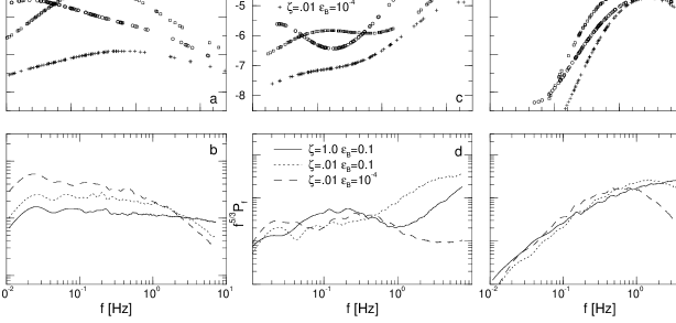
Fig. 1.—: Upper panels: the fraction of the wind energy radiated by a pulse in the 50–300 keV band as function of pulse duration. Parameters: redshift $z=1$, $\eta_{m}=30$, $\varepsilon_{e}=0.25$, $p=2.5$, $t_{w}=20$ s, $t_{v}=20$ ms ($N=10^{3}$ shells). Only a small fraction of the total number of pulses is shown; the density of the points illustrates the pulse duration distribution. The curves shown are log-log space fits for the most efficient pulses. The actual values are scattered around the fit. Lower panels: the corresponding PDS (note that $f^{5/3}P_{f}$ is plotted in panels 1$d$ and 1$f$), calculated by averaging the PDSs of 100 bursts in each case, all bursts having the same parameters. Panels 1$a$ and 1$b$: optically thin uniform winds, panels 1$c$ and 1$d$: optically thin modulated winds; for both cases $\eta_{M}=1000$ and $L_{w}=10^{53}\,\rm{erg\,s^{-1}}~{}$. Panels 1$e$ and 1$f$: quasi-optically thick uniform winds ($\eta_{M}=300$, $L_{w}=10^{54}\,\rm{erg\,s^{-1}}~{}$). Other parameters are given in the legend.

Fig. 2.—: Effect of $L_{w}$ and $z$ on the PDS of optically thin modulated winds. The solid thick line shows the features (i.e. only trends, the ordinate values depend on the choice of normalization) of the PDS obtained by BSS98 for real bursts. Other parameters: $\zeta=10^{-2}$, $\varepsilon_{e}=0.25$, $p=2.5$, $\varepsilon_{B}=10^{-6}$, $\eta_{m}=30$, $\eta_{M}=1000$, $t_{w}=20$ s, $t_{v}=20$ ms. Each PDS is the average of 250 power spectra of simulated bursts.

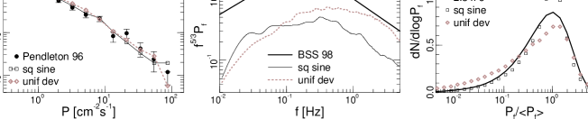
Fig. 3.—: Intensity distribution (panel $a$), average power density spectrum (panel $b$) and distribution of $P_{f}$ around the average PDS (panel $c$) for two models: $\sin^{2}$-modulated wind (squares or solid curve) and uniform wind (diamonds or dotted curve). The winds have a power-law luminosity distribution and an un-evolving rate density. The mean redshift and dispersion of the bursts brighter than $1\,\gamma\,{\rm cm^{-2}s^{-1}}~{}$ are $z=1.24$, $\sigma_{z}=0.91$ for the modulated wind model and $z=0.94$, $\sigma_{z}=0.84$ for the uniform wind model. The former model has $L_{m}=7\times 10^{52}\,\rm{erg\,s^{-1}}~{}$, $\eta_{M}=1000$, $\varepsilon_{B}=10^{-6}$, $\zeta=10^{-2}$, the latter is characterized by $L_{m}=8\times 10^{53}\,\rm{erg\,s^{-1}}~{}$, $\eta_{M}=220$, $\varepsilon_{B}=10^{-4}$, $\zeta=1$. Other parameters are $L_{M}/L_{m}=100$, $\beta=2$, $\eta_{m}=30$, $t_{w}=20$ s, $t_{v}=20$ ms, $\varepsilon_{e}=0.25$, $p=2.5$, for both models.

Fig. 4.—: Typical 50–300 keV light-curves of the bursts whose PDSs are shown in Figure 3, within the two models for ejection LFs: panel $a$ – modulated wind with $L_{w}=10^{53}\,\rm{erg\,s^{-1}}~{}$, panel $b$ – uniform wind with $L_{w}=10^{54}\,\rm{erg\,s^{-1}}~{}$. Both bursts are placed at redshift $z=1$. Other parameters are as for Figure 3.