Velocity distribution of stars in the solar neighbourhood

Abstract

A two-dimensional velocity distribution in the $UV$-plane has been obtained for stars in the solar neighbourhood, using the Hipparcos astrometry for over 4000 ‘survey’ stars with parallaxes greater than 10 mas and radial velocities found in the Hipparcos Input Catalogue. In addition to the already known grouping characteristics (field stars plus young moving groups), the velocity distribution seems to exhibit a more complex structure characterized by several longer branches running almost parallel to each other across the $UV$-plane. By using the wavelet transform technique to analyse the distribution, the branches are visible at relatively high significance levels of 90 per cent or higher. They are roughly equidistant with a separation of about 15 $\mbox{km}\,\mbox{s}^{-1}$ for early-type stars and about 20 $\mbox{km}\,\mbox{s}^{-1}$ for late-type stars, creating an overall quasi-periodic structure which can also be detected by means of a two-dimensional Fourier transform. This branch-like velocity distribution might be due to the galactic spiral structure.

1 Introduction

The velocity distribution of stars in the solar neighbourhood is an important tool for studying different aspects of galactic kinematics and dynamics. During a long era of ground-based astrometry that preceded the Hipparcos mission, many subtle details in the velocity field have gone undetected due to the smearing caused by large uncertainties in stellar parallaxes. With the Hipparcos measurements we are in a position to investigate the structure in more detail, confirming some previous characteristics and discovering some new features.

A typical analysis of the distribution of stars in the $UV$-plane concentrates on determining the velocity ellipsoid and its parameters (dispersions in $U$, $V$ and $W$, as well as the orientation of the principal axis, i.e. the longitude of the vertex). More details about this can be found in any textbook on galactic structure and kinematics (e.g. Mihalas & Binney 1981). In addition to the global properties of the velocity ellipsoid, a variety of different local irregularities are also studied. Certain concentrations of stars in velocity space mean that there exist groups of stars (moving groups) that move with the same velocity. This idea has been elaborated extensively in works by Eggen (e.g. 1970) and other authors. Different authors use different techniques and different stellar samples, but they all report the presence of moving groups in the solar neighbourhood (Figueras et al. 1997, Chereul et al. 1997,1998,1999, Dehnen 1998, Asiain et al. 1999).

This paper is part of a larger project started at the University of Canterbury in order to test Eggen’s hypothesis (Skuljan et al. 1997). Here we discuss some inhomogeneities in the velocity distribution that are related to moving groups and can give some clues to the problem of star formation.

2 The sample

For this study a sample of 4597 stars has been constructed using the following selection criteria:

1. Parallax greater than 10 mas (stars within 100 pc of the Sun), and $\sigma_{\pi}/\pi<0.1$, as taken from the Hipparcos Catalogue (ESA 1997).

2. Survey flag (Hipparcos field H68) set to ‘S’.

3. Existing radial velocities in the Hipparcos Input Catalogue (ESA 1992).

4. Existing $B-V$ colours in the Hipparcos Catalogue.

The survey flag has been used so that no stars proposed by various individual projects are included in this analysis, since they could introduce a bias. Stars with parallax uncertainties greater than 10 per cent have been rejected in order to have a reliable error propagation. The Hipparcos $B-V$ colour index is used here as a suitable indicator for dividing the sample into two subsets, as explained in Section 6.

There are 12520 ‘survey’ stars with parallaxes greater than 10 mas, out of 118218 entries found in the Hipparcos Catalogue. However, only 11009 of these stars have their parallax uncertainties less than 10 per cent. Finally, for 11007 of them the $B-V$ colours are known. On the other hand, we find 19467 stars with known radial velocities, out of 118209 entries in the Hipparcos Input Catalogue. Only 4597 stars are found in both subsets, if the catalogue running numbers are used as a matching criterion ($\mbox{HIP}=\mbox{HIC}$).

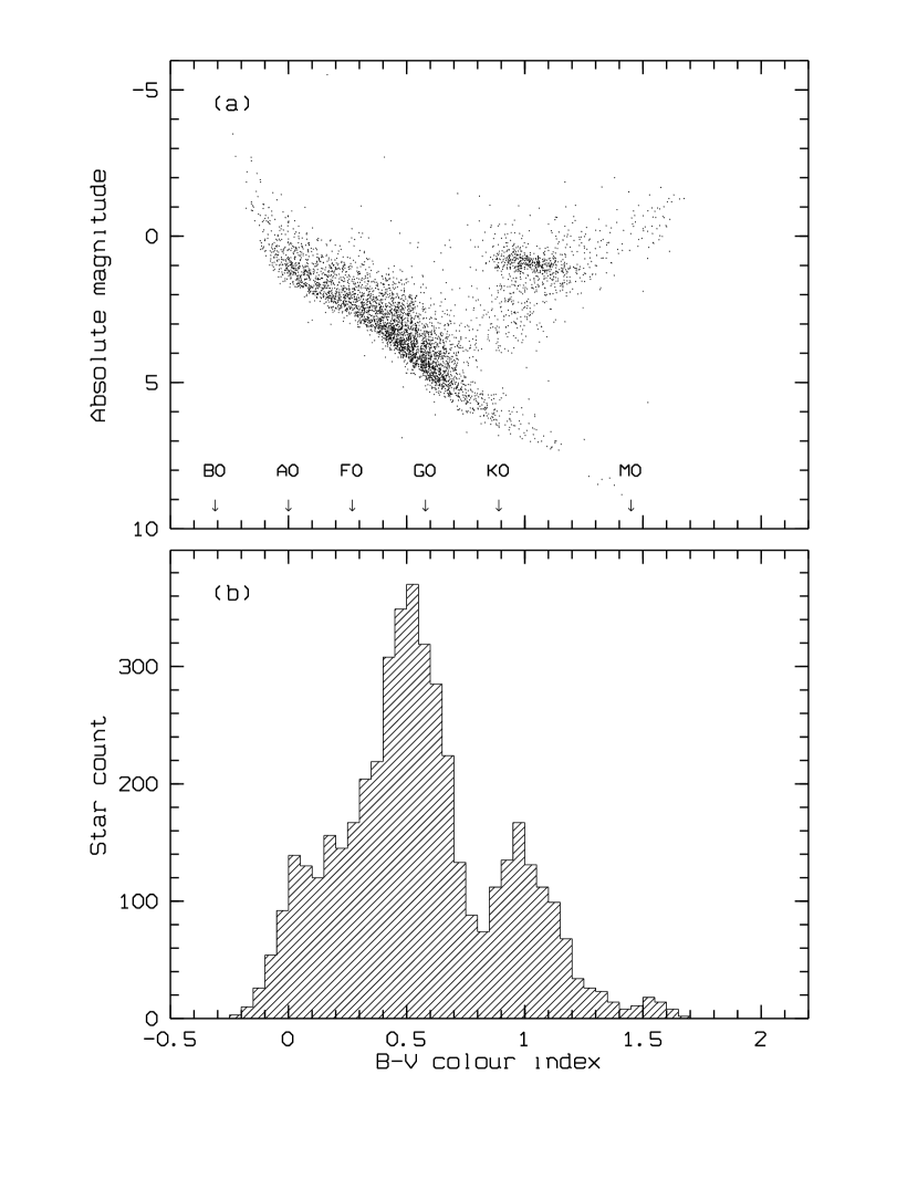
Figure 1: H-R diagram of the 4597 Hipparcos ‘survey’ stars within 100 pc, with known radial velocities and colours (a) and the distribution of the $B-V$ colour index (b). The spectral classes (a) correspond to the main sequence (Allen 1991).

Before we proceed with our analysis of the velocity distribution, some important points have to be emphasized here concerning the problem of bias. First of all, not all spectral classes are equally represented in our sample. The Hipparcos catalogue is essentially magnitude limited, which means that we shall have a significant deficiency of red dwarfs, compared to the young early-type stars. The situation is illustrated in Figure 1. A great majority of stars are concentrated around $B-V=0.5$, corresponding to the main-sequence F stars. There is also a possible concentration of earlier-type stars around A0, as well as a distinct peak of K giants (red-clump stars on the horizontal branch, to be more precise) around $B-V=1.0$. This should be kept in mind when drawing any conclusions regarding the stellar ages (see Section 6), but it will essentially not affect our results.

A possibly more serious problem concerning our stellar sample is a kinematic bias. Binney et al. (1997) demonstrated that radial velocities are predominantly known for high-proper-motion stars. If only the stars with known radial velocities are used, then any velocity distribution derived from such a biased sample might give a false picture and lead to some wrong conclusions about the local stellar kinematics. That is the reason why many authors today choose not to include the measured radial velocities at all (see also Dehnen & Binney 1998, Dehnen 1998, Crézé et al. 1998, Chereul et al. 1998,1999).

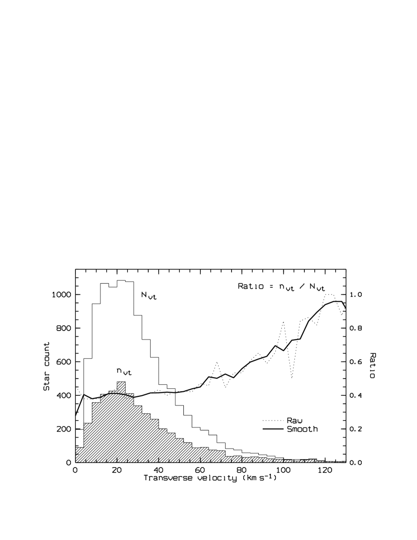
Figure 2: Kinematic bias, presented as a ratio between two distributions: stars with known radial velocities ($n_{v_{\rm t}}$) out of the total sample of Hipparcos ‘survey’ stars within 100 pc ($N_{v_{\rm t}}$), where $v_{\rm t}$ is the transverse velocity. Radial velocities are predominantly known for high-$v_{\rm t}$ stars, but the effect is important only at $v_{\rm t}>70-80\ \mbox{km}\,\mbox{s}^{-1}$.

We have checked for potential kinematic bias in our case, and the result is presented in Figure 2. Two distributions are shown as functions of the transverse velocity ($v_{\rm t}=4.74\,\mu/\pi$), one for the total sample of 11007 ‘survey’ stars within 100 pc ($N_{v_{\rm t}}$), and the other for the stars with known radial velocities only ($n_{v_{\rm t}}$). The $v_{\rm t}$-axis has been divided into 4-$\mbox{km}\,\mbox{s}^{-1}$ bins and the stars have been counted in each bin. If there was no kinematic bias, then the probability that a star has a radial velocity should be constant from bin to bin, and the ratio $n_{v_{\rm t}}/N_{v_{\rm t}}$ would appear as a flat line. It is obvious from Figure 2 that this is not the case for our sample. While the radial velocities are known for about 40 per cent of the stars at $v_{\rm t}=20\ \mbox{km}\,\mbox{s}^{-1}$, the ratio reaches 80 per cent at $v_{\rm t}=120\ \mbox{km}\,\mbox{s}^{-1}$. However, the effect becomes a real problem only at higher velocities, above 70 – 80 $\mbox{km}\,\mbox{s}^{-1}$, as easily seen from the diagram. Below this limit, the ratio stays more or less flat, so that we can expect no significant distortions in the inner parts of the velocity distribution, where we shall primarily concentrate our attention. We shall return to this problem again when we compare our velocity distribution to those of other authors (see Section 3).

3 Velocity distribution

Having fixed the stellar sample, we can now proceed with the analysis. Hipparcos parallaxes and proper motions, together with the radial velocities from the Hipparcos Input Catalogue, have been used to compute the stellar space velocities relative to the Sun. The right-handed coordinate system has been used, with the $X$-axis pointing towards the galactic centre, $Y$-axis in the direction of galactic rotation (clockwise, when seen from the north galactic pole), and $Z$-axis towards the north galactic pole. Corresponding velocity components are $U$, $V$ and $W$ respectively. A typical error-bar in each velocity component is close to $1\ \mbox{km}\,\mbox{s}^{-1}$, with about 80 per cent of stars having their velocity uncertainties less than $2\ \mbox{km}\,\mbox{s}^{-1}$, as shown in Fig. 3. The error propagation has been treated taking into account the full correlation matrix between the Hipparcos astrometric parameters.

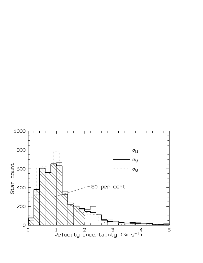
Figure 3: The distribution of the uncertainties in all three velocity components: $\sigma_{U}$ (thin line), $\sigma_{V}$ (bold line) and $\sigma_{W}$ (dotted line). The uncertainty is less than $2\ \mbox{km}\,\mbox{s}^{-1}$ for about 80 per cent of stars.

In order to estimate the probability density function $f(U,V)$ from the observed data, we use here an adaptive kernel method (for more details see Silverman 1986). The basic idea of this method is to apply a smooth weight function (called the kernel function) to estimate the probability density at any given point, using a number of neighbouring data points. The term ‘adaptive’ here means that the kernel width depends on the actual density, so that the smoothing is done over a larger area if the density is smaller.

We use the following definition of the adaptive kernel estimator (see page 101 of Silverman 1986), defined at an arbitrary point $\vec{\xi}=(U,V)$:

$$\hat{f}(\vec{\xi})=\frac{1}{n}\sum\limits_{i=1}^{n}\frac{1}{h^{2}\lambda_{i}^{2}}K\left(\frac{\vec{\xi}-\vec{\xi}_{i}}{h\lambda_{i}}\right)$$

where $K(\vec{r})$ is the kernel function, $\lambda_{i}$ are the local bandwidth factors (dimensionless numbers controlling the overall kernel width at each data point), and $h$ is a general smoothing factor. We assume also that there are $n$ data points $\vec{\xi}_{i}=(U_{i},V_{i})$. Our function $K(\vec{r})$ is a 2-D radially symmetric version of the biweight kernel (Fig. 4), and is defined by:

$$K(r)=\left\{\begin{array}[]{ll}\frac{3}{\pi}(1-r^{2})^{2},&r<1\\ 0,&r\geq 1\end{array}\right.$$

so that $\int K(\vec{r})d\vec{r}=1$ (a condition that any kernel must satisfy in order to produce an estimate $\hat{f}$ as a proper probability density function).

Figure 4: Kernel function $K(r)$ used for the probability density estimation.

The local bandwidth factors $\lambda_{i}$ needed for the computation of $\hat{f}(\vec{\xi})$ are defined by:

$$\lambda_{i}=\left[\frac{\hat{f}(\vec{\xi}_{i})}{g}\right]^{-\alpha}$$

where $g$ is the geometric mean of the $\hat{f}(\vec{\xi}_{i})$:

$$\ln g=\frac{1}{n}\sum\limits_{i=1}^{n}\ln\hat{f}(\vec{\xi}_{i})$$

and $\alpha$ is a sensitivity parameter, which we fix at $\alpha=0.5$ (a typical value for the two-dimensional case). Note that in order to compute $\lambda_{i}$ we need the distribution estimate $\hat{f}$ which, in turn, can be computed only when all $\lambda_{i}$ are known. This problem, however, can be solved iteratively, by starting with an approximate distribution (a fixed kernel estimate, for example), and then improving the function as well as the $\lambda_{i}$ factors in a couple of subsequent iterations.

Finally, an optimal value for the smoothing parameter $h$ is determined using the least-squares cross-validation method, by minimizing the score function:

$$M_{o}(h)=\int\!\!\hat{f}^{2}\ -\ \frac{2}{n}\sum\limits_{i=1}^{n}\hat{f}_{-i}(\vec{\xi}_{i})$$

where $\int\!\!\hat{f}^{2}$ can be computed numerically, and $\hat{f}_{-i}(\vec{\xi}_{i})$ is the density estimate at $\vec{\xi}_{i}$, constructed from all data points except $\vec{\xi}_{i}$. It can be shown that minimizing $M_{o}(h)$ is equivalent (in terms of mathematical expectation) to minimizing the integrated square error $\int(\hat{f}-f)^{2}$, so that our estimate $\hat{f}$, based on the optimal value for $h$, is as close as possible to the true distribution $f$, using the data set available. In our case (for the whole sample of stars), we have found the minimum of $M_{o}(h)$ at $h=10.7\ \mbox{km}\,\mbox{s}^{-1}$.

Our $UV$-distribution of stellar velocities with respect to the Sun is shown in Fig. 5, both as a scatter plot and a smooth contour plot representing the density function $\hat{f}(U,V)$, as computed using the adaptive kernel method described above. The computations have been performed on a grid of square bins of $2\times 2$ $\mbox{km}\,\mbox{s}^{-1}$. This choice for the bin size has been made taking into account a typical uncertainty in the velocity components, as mentioned earlier (Fig 3). Finally, the density function has been rescaled by a multiplication factor $nS$, where $n=4597$ is the total number of stars and $S=4$ $\mbox{km}^{2}\,\mbox{s}^{-2}$ is the area covered by a square bin. The numerical value of the transformed distribution at any given bin is therefore equal to the average number of stars falling in that bin (assuming that our estimate $\hat{f}$ is close to the real distribution $f$).

The distribution in Fig. 5 is obviously not uniform, showing some concentrations that have been associated with the Hyades, Pleiades, Sirius and other young moving groups (see e.g. Figueras et al. 1997, Chereul et al. 1997). A closer examination, however, reveals an additional pattern of inhomogeneities on a somewhat larger scale. At least three long branches (we shall call them: the Sirius branch, the middle branch and the Pleiades branch, respectively from top to bottom) can be identified by eye, slightly curved but almost parallel and running diagonally across the diagram with a negative slope. We have traced the branches in a preliminary way by following the local maxima (ridge lines) in the $UV$-distribution, as shown by the dashed lines in Fig. 5.

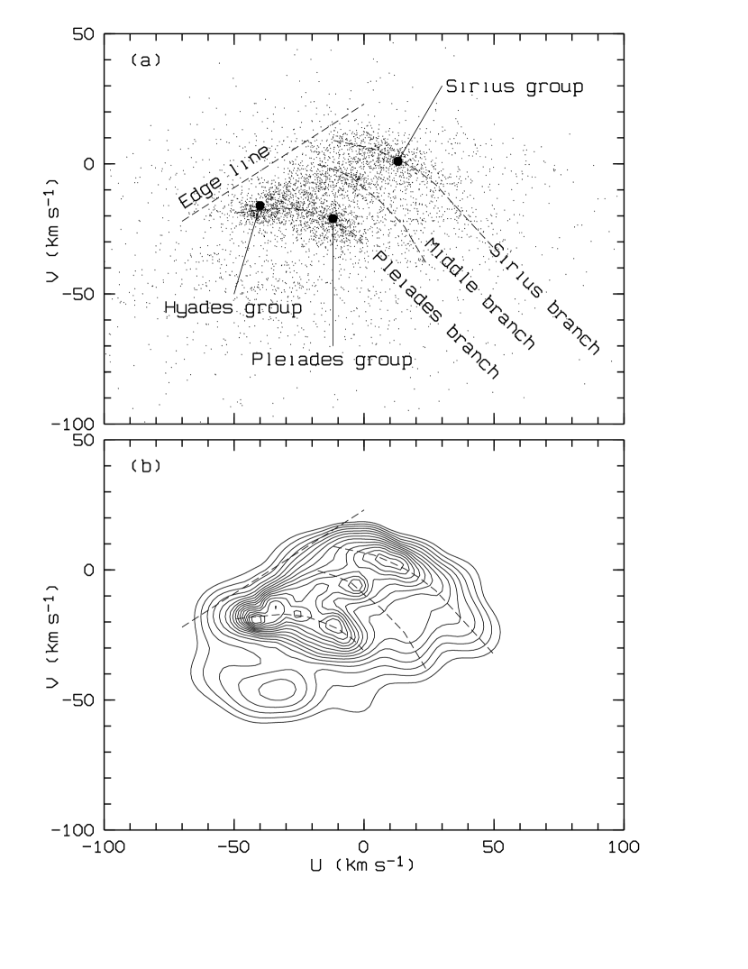
Figure 5: The distribution of stellar velocities in the $UV$-plane, shown as a scatter plot (a), and a contour plot of the probability density function (b) in logarithmic scale. The density function has been obtained using the adaptive kernel method (see text). The three main moving groups (a) are marked as filled circles. The three hypothetical branches and the ’edge line’ are shown as dashed lines.

It has been pointed out before (Skuljan et al. 1997) that the parallax uncertainty can produce some radially-elongated features in the $UV$-plane, since the stars tend to move radially relative to the zero point ($U=0$, $V=0$) when their parallax is changed. However, this effect would create some branches converging to the zero point, which is clearly not the case in Fig. 5. We conclude that the parallax uncertainty cannot be responsible for the distribution found.

Besides the three branches, there seems to exist a fairly sharp ‘edge line’ at an angle of about $+30^{\circ}$ relative to the $U$-axis, connecting the lower-$U$ extremities of the branches and defining a region above the line where only a few stars can be found. Practically all the stars seem to occupy the lower part of the $UV$-plane bounded by the ‘edge line’ and the Sirius branch. In such a situation, the traditional velocity-ellipsoid approach does not seem to be appropriate any more.

It would be interesting to compare our distribution from Fig 5 to similar diagrams obtained by other authors (Asiain et al. 1999, Chereul et al. 1998,1999, Dehnen 1998). In particular, Fig. 3 of Dehnen 1998 demonstrates all basic features that we introduce here, although their distribution was obtained without radial velocities. This clearly suggests that the kinematic bias (Binney et al. 1997) does not affect significantly the inner parts of the $UV$-distribution.

4 The wavelet transform

In order to determine the precise nature and the statistical significance of the features seen in Fig. 5 we have chosen the wavelet transform technique to analyse our data. There are many examples in the literature demonstrating how this powerful tool can be used in different areas (e.g. Slezak et al. 1990, Chereul et al. 1997), but nevertheless we shall point out some of the basic properties relevant to our work, concentrating on the two-dimensional case only.

To do a wavelet transform of a function $f(x,y)$ we define a so-called analysing wavelet $\psi(\frac{x}{a},\frac{y}{a})$, which is another function (or another family of functions), where $a$ is the scale parameter. By fixing the scale parameter we can select a wavelet of a given particular size out of a family characterized by the same shape $\psi$. The wavelet transform $w(x,y)$ is then defined as a correlation function, so that at any given point ($\xi,\eta$) in the $XY$-plane we have one real value for the transform:

$$w(\xi,\eta)=\int\limits_{-\infty}^{\infty}\int\limits_{-\infty}^{\infty}f(x,y)\,\psi(\frac{x-\xi}{a},\frac{y-\eta}{a})\,dx\,dy,$$

which is called the wavelet coefficient at ($\xi,\eta$). Since we usually work in a discrete case, having a certain finite number of bins in our $XY$-plane, this means that we shall have a finite number of wavelet coefficients, one value per bin.

The actual choice of the analysing wavelet $\psi$ depends on the particular application. When a given data distribution is searched for certain groupings (over-densities) then a so-called Mexican hat is most commonly used (e.g. Slezak et al. 1990). A two-dimensional Mexican hat (Fig. 6) is given by:

$$\psi(r/a)=\left(2-\frac{r^{2}}{a^{2}}\right)e^{-{r^{2}}/{2a^{2}}}$$

where $r^{2}=x^{2}+y^{2}$. The main property of the function $\psi$ is that the total volume is equal to zero, which is what enables us to detect any over-densities in our data distribution. The wavelet coefficients will be all zero if the analysed distribution is uniform. But if there is any significant ‘bump’ in the distribution, the wavelet transform will give a positive value at that point. Moreover, if we normalize the Mexican hat using a factor $a^{-2}$, then we will be able to estimate the half-width of the ‘bump’, by simply varying the scale parameter $a$: the wavelet coefficient in the centre of the bump will reach its maximum value if the scale $a$ is exactly equal to $\sigma$, assuming that the ‘bump’ is a gaussian of a form: $\exp(-\rho^{2}/2\sigma^{2})$, $\rho$ being the distance from the centre.

Many authors choose the scale in such a way that it gives the maximum wavelet transform. This is an attractive option providing straightforward information on the average half-width of the gaussian components in our distribution. However, there are some situations when we would prefer somewhat smaller scales, in order to separate two close components or to detect some narrow but elongated features.

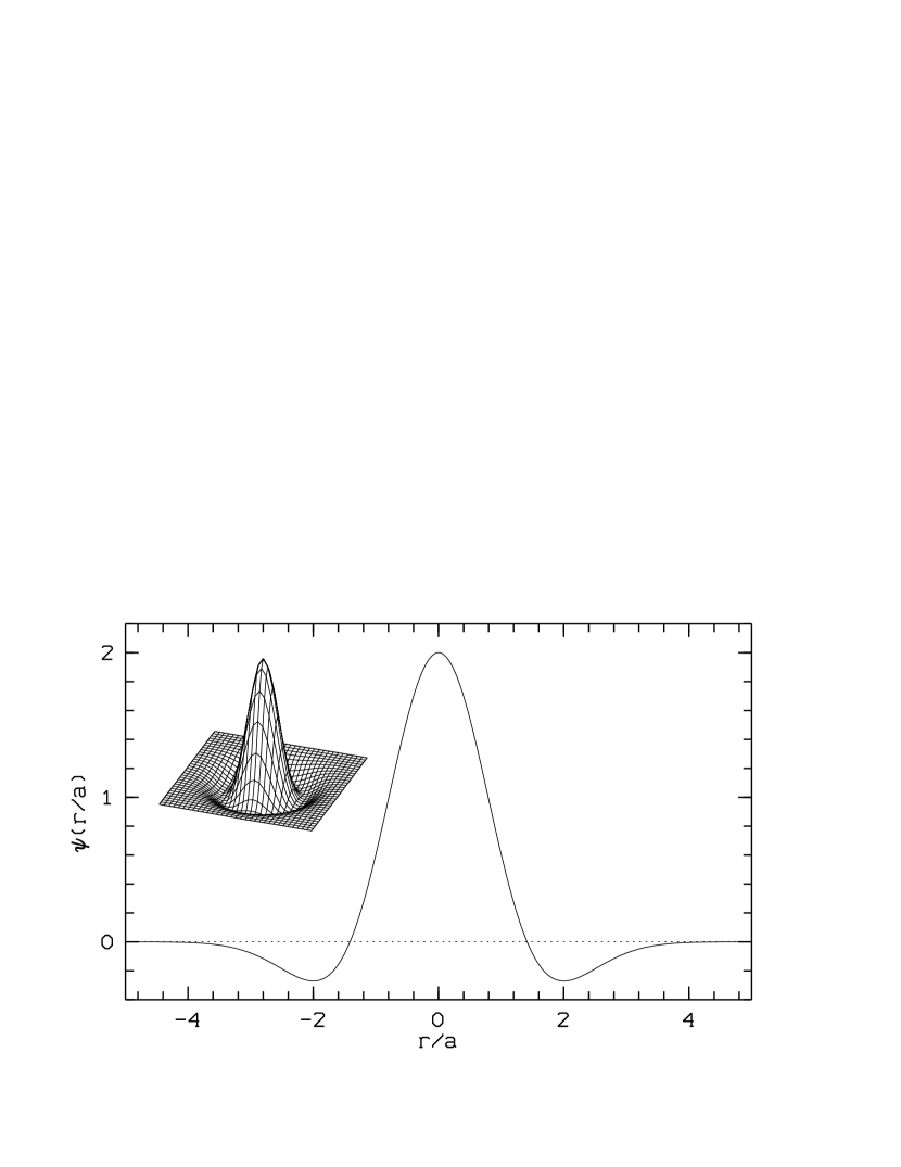
Figure 6: The Mexican hat in two dimensions.

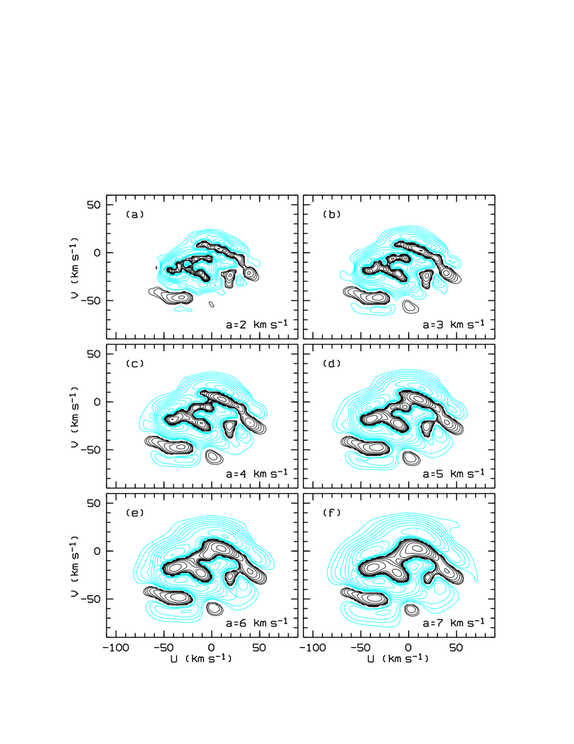
Figure 7: Wavelet transforms of the smooth $UV$-distribution at several different scales. Solid lines represent positive contours, while dashed lines are used for negative values.

We have applied several different scales to our $UV$-distribution from Fig. 5b, and the results are shown in Fig. 7. The positive contours (solid lines) describe the regions where we have an over-density of stars (grouping), while the negative contours (dashed lines) show the regions with star deficiency (under-density). We shall concentrate our attention here only on the positive values. At about $a\sim 4-5$ $\mbox{km}\,\mbox{s}^{-1}$ the normalized wavelet coefficients reach their maxima around the most populated parts of the $UV$-plane (except the Hyades moving group, where the maximum wavelet transform occurs somewhere below $2$ $\mbox{km}\,\mbox{s}^{-1}$, i.e. at a scale less than the bin size).

5 Confidence levels

An important question at this stage is how probable are the features revealed in Fig. 7, i.e. what are the confidence levels for the contours to be above the random noise. A commonly used procedure to estimate the probabilities is numerical simulation (sometimes called the Monte Carlo method) based on random number generators (see e.g. Escalera & Mazure 1992).

Let us consider again the distribution in Fig. 5b. By smoothing the probability density function we have found the average number of stars $\bar{N}_{\ast}$ in each bin (to be more precise, we have found an optimal estimate of the average value, as close as possible using the data set available). On the other hand, the observed number of stars $N_{\ast}$ in each bin has a statistical uncertainty. This is not only due to the measurement errors. Even if the velocities have no random errors (or extremely small errors, i.e. much less than the bin size) we still have statistical fluctuations related to the finite sample. We can expect that the observed number of stars $N_{\ast}$ in each bin will fluctuate following the Poisson distribution, with an average of $\bar{N}_{\ast}$. This means that we can regard our observed histogram as one outcome from an infinite set of possibilities, when we let the star counts in every bin fluctuate according to the Poisson statistics. We can numerically simulate those “other possibilities” and create the distributions (copies) that “could have happened”. If any feature of the distribution is found repeating from one copy to another, we can be confident that the feature is real, i.e. not generated by noise. Actually, the number of successful appearances divided by the total number of simulations will give us the probability of the feature being real.

We use this idea to find the probabilities that our wavelet coefficients are positive, since a positive coefficient is automatically an indicator that a grouping in the $UV$-plane exists. We generate a large number ($N=1000$) of Poisson random copies of our smooth histogram from Fig. 5b. Then, for each of these copies, we derive a replica of the original data set, by creating $N_{\ast}$ stars randomly distributed over each bin (in total, we shall have a number of stars close to $n=4597$ for all bins together). Finally, we treat the new data set in the same way as the original: we estimate the density function by applying the adaptive kernel method, and then compute the wavelet transform of the corresponding smooth histogram. This enables us to examine each coefficient ($w$) over the whole set of simulations, and compute the probability such that the value is positive. If there are $N_{\rm p}$ simulations with $w>0$ then we have a probability $P(w>0)=N_{\rm p}/N$. This procedure has been repeated for all wavelet transforms that we shall present in this paper. Typically, the features shown have a 90 per cent or better probability of being real.

6 The data analysis

Although we have started our analysis by examining the whole sample of stars, we are aware of the fact that the stellar kinematic properties may depend on the age. It is reasonable to assume that younger stars have better chances of still keeping the memory of their original velocities that they acquired at formation. If there is any grouping in velocity space, and if the grouping is only a result of cluster evaporation (Eggen’s hypothesis), then we would expect to see it most prominently amongst the youngest stars.

In this paper we are not dealing explicitly with the stellar ages but we are using the spectral type (colour index actually) as an age indicator. We have divided the whole sample of stars into two groups:

1. 1036 early-type stars ($B-V<0.3$), and

2. 3561 late-type stars ($B-V>0.3$).

by choosing $B-V=0.3$ as an arbitrary division point, corresponding approximately to the boundary between the A and F spectral classes. The terms ‘early-type’ and ‘late-type’ should be regarded here as suitable names to be used in this paper only. Note that our late-type group contains spectral classes F and later, with two distinct clumps (main sequence F stars, plus K giants) as seen in Fig. 1. Analysing the Hipparcos catalogue, Dehnen & Binney (1998) found Parenago’s discontinuity at $B-V=0.61$, which means that most of the stars blue-ward of that are younger than the Galactic disk itself. This applies to the F stars in our sample. We can conclude that our early-type group (spectral classes B–F) contains predominantly young stars, while our late-type group (F–M) is a mixture of older and younger main-sequence stars, rather young red-clump stars, and a few old red giants. The first group should better show the young moving groups and it will allow us to compare the results with other authors. On the other hand, the second group should possibly show the old-disk moving groups that can be compared with Eggen’s results.

6.1 Early-type stars

We have applied the adaptive kernel method again to derive the probability density function $f(U,V)$ for the 1036 early-type stars. An optimal value for the smoothing parameter in this case is $h=8.1$ $\mbox{km}\,\mbox{s}^{-1}$. The smooth distribution, together with the corresponding wavelet transforms at several different scales, are shown in Fig 8. The three branches are well separated and easily detected. Although the ‘middle branch’ does not appear as a feature sufficiently long for a separate analysis, we shall nevertheless treat it as an ‘incomplete’ branch. The maximum wavelet transform is at about $a=4\ \mbox{km}\,\mbox{s}^{-1}$, which also corresponds to an average half-width of the branches.

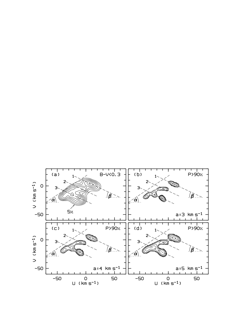
Figure 8: The velocity distribution of early-type stars (a) together with the corresponding wavelet transforms (90 per cent confidence) at several different scales (b–d). The dashed lines are used to mark the branches and the edge line (see text for equations of lines).

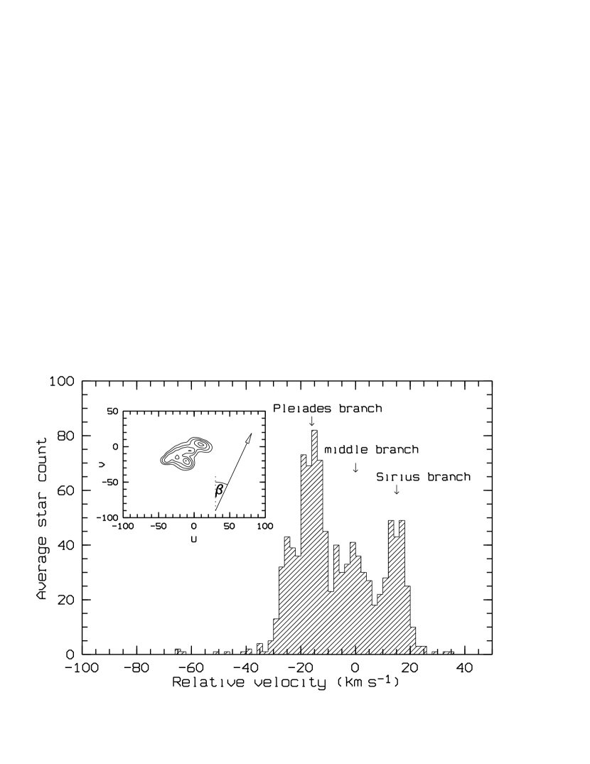
Figure 9: The one-dimensional velocity distribution of early-type stars along an axis perpendicular to the branches (the direction indicated in the inserted image).

In order to determine the edge line we have used the 5-per-cent level (relative to the maximum) of the smoothed $UV$-histogram, as indicated in Fig. 8a. By fitting a straight line to the corresponding portion of the contour we find the tilt to be $\alpha\approx 32^{\circ}$ ($\tan\alpha\approx 0.62$) and the edge line to follow the equation $V=16.4\ \mbox{km}\,\mbox{s}^{-1}+0.62U$.

The tilt of the branches (assuming that they all have the same tilt) has been computed by rotating the wavelet transform (Fig. 8b) counter-clockwise and examining the distribution along $V$ only (taking a sum of all positive wavelet coefficients at a given $V$). At an angle of $\beta\approx 25^{\circ}$ ($\tan\beta\approx 0.47$) the three branches appear as the narrowest (and strongest) gaussians, which means that the tilt of the branches in the $UV$-plane is $-25^{\circ}$. We find the following three equations for the branches, which are shown in Fig 8:

$$V_{1}= 7.6\ \mbox{km}\,\mbox{s}^{-1}-0.47U$$ (Sirius branch)

$$V_{2}= -8.9\ \mbox{km}\,\mbox{s}^{-1}-0.47U$$ (middle branch)

$$V_{3}= -26.6\ \mbox{km}\,\mbox{s}^{-1}-0.47U$$ (Pleiades branch)

It should be noted, however, that these three linear relations describe the branches well enough only relatively far from the edge line. The branches seem to curve and follow the edge line at their lower-$U$ extremity. This is especially the case with the Pleiades branch.

In Fig. 9 we present the one-dimensional distribution in the direction perpendicular to the branches ($\beta\approx 25^{\circ}$) so that each branch appears as a single peak at a fixed position. The zero point of the relative velocity scale has been centred on the middle branch. The three branches are approximately equidistant, with a separation of about $15\ \mbox{km}\,\mbox{s}^{-1}$.

6.2 Late-type stars

The distribution function in the $UV$-plane for the 3561 late-type stars has been computed using an optimal smoothing factor of $h=13.6$ $\mbox{km}\,\mbox{s}^{-1}$. The contour diagrams of the distribution and the corresponding wavelet transforms at several different scales, are shown in Fig 10. If we compare this with the early-type case in Fig. 8, we find a similar pattern, although somewhat more complex. Besides the three main branches, we have now got some new details, such as a concentration of stars at about $(20,-30)$ $\mbox{km}\,\mbox{s}^{-1}$ (possibly another fragment of the middle branch), as well as a new branch in the bottom part of the diagram, at $(-30,-50)$ $\mbox{km}\,\mbox{s}^{-1}$. In order to get the new features named, we introduce here two of Eggen’s old-disk moving groups, Wolf 630 and $\zeta$ Herculis, also marked in Fig. 10d. We shall simply use the fact that these two Eggen’s moving groups (Eggen 1965,1971) agree well with the features revealed by our wavelet transforms, although the question of the significance of such a correlation is still to be answered.

In order to find the positions of the branches in Fig. 10, we could perhaps proceed as when dealing with the early-type stars. However, the branches now seem longer, and possibly curved (especially the Sirius branch), so that our procedure for determining the angle $\beta$ does not seem to be appropriate any more. On the other hand, there is not enough data to do a more sophisticated analysis including the curvature of the detected features. Our approach was to adopt the same inclination angle of $\beta\approx 25^{\circ}$, as derived from the early-type stars, and then simply find the positions of the branches from the rotated one-dimensional distribution shown in Fig. 11. The equations for the branches are:

$$V_{1}= 6.9\ \mbox{km}\,\mbox{s}^{-1}-0.47U$$ (Sirius branch)

$$V_{2}= -7.0\ \mbox{km}\,\mbox{s}^{-1}-0.47U$$ (middle branch)

$$V_{3}= -29.2\ \mbox{km}\,\mbox{s}^{-1}-0.47U$$ (Pleiades branch)

$$V_{4}= -62.0\ \mbox{km}\,\mbox{s}^{-1}-0.47U \zeta$$ ( Herculis branch)

There is also a possible hint of a weak fifth branch (Fig. 11) at a relative velocity of about 30 $\mbox{km}\,\mbox{s}^{-1}$. An overall impression is that the branches are roughly equidistant, with a separation slightly larger than in the early-type stars. With one additional branch, an average separation is now about 20 $\mbox{km}\,\mbox{s}^{-1}$. If this ‘periodicity’ is real, then a two-dimensional Fourier transform of the distribution will show some peaks in the power spectrum, as we shall demonstrate in the following section.

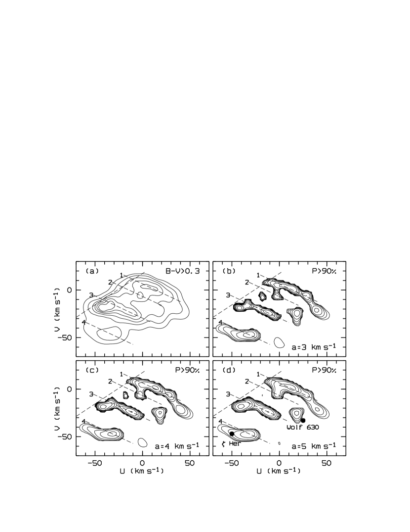
Figure 10: The velocity distribution of late-type stars (a) and the corresponding wavelet transforms (90 per cent confidence) at several different scales (b–d). The dashed lines are used to mark the branches and the edge line (see text for equations). Two Eggen’s old-disk moving groups (d) are presented for reference.

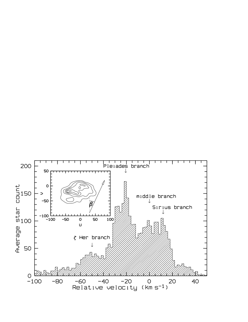
Figure 11: The one-dimensional velocity distribution of late-type stars along an axis perpendicular to the branches (the direction indicated in the inserted image).

7 The Fourier transform

The two-dimensional power spectrum $Q(f_{U},f_{V})$ of the smooth $UV$-histogram for the whole sample of stars (square root of the power spectral density) is shown in Fig. 12. Most of the total power is concentrated within the central bulge (maximum power density of about 4700), corresponding to a roughly gaussian distribution of the stars in the $UV$-plane. There are also two relatively strong side peaks (maximum power density of about 920) symmetrically arranged around the central bulge at frequencies ($\pm 0.008,\pm 0.031$) $\mbox{s}\,\mbox{km}^{-1}$, as well as two higher harmonics at ($\pm 0.016,\pm 0.054$) $\mbox{s}\,\mbox{km}^{-1}$. The peaks are arranged along a straight line at an angle of $\gamma=74^{\circ}$ (the dashed line in Fig. 12a). Some other features can also be seen at relatively high significance levels, but we shall concentrate here only on the aligned peaks. They define a planar wave in the velocity plane. Of course, the peaks at negative frequencies are simply symmetrical images of the positive ones, without any additional information.

In order to estimate the significance of the features in the power spectrum, we have proceeded in a similar way as when treating the wavelet transforms. A large number of random copies have been used to see how the power spectral density fluctuates at any given frequency point. The standard deviation $\sigma$, has been computed for each bin and the ratio $Q/\sigma$ has been used as a measure of significance.

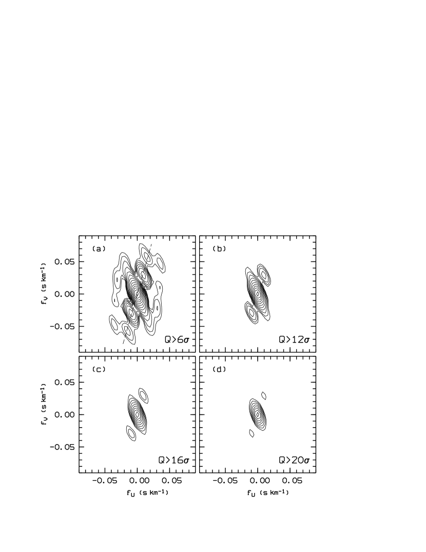
Figure 12: The two-dimensional power spectrum $Q(f_{U},f_{V})$ of the velocity distribution for the whole sample of stars, at several levels of significance. The strongest peaks are aligned at $\gamma\approx 74^{\circ}$, as indicated by the dashed line (a).

Every peak in the power spectrum can be related to a planar wave propagating in a certain direction, with a frequency $f=\sqrt{f_{U}^{2}+f_{V}^{2}}$. We find a period of about 33 $\mbox{km}\,\mbox{s}^{-1}$ for the stronger side peak (the one closer to the central bulge), and about 17 $\mbox{km}\,\mbox{s}^{-1}$ for the first harmonic. These values are in a good agreement with our wavelet transform analysis: the longer period corresponds to the separation between the two most prominent branches in the $UV$-distribution (Sirius and Pleiades), while the second one can be related to the remaining weaker branches. It should be noted, however, that the power spectrum contains obviously much more information than we have extracted here, and a more detailed analysis is needed.

8 Conclusion

Using the Hipparcos astrometry and published radial velocities, we have undertaken a detailed examination of the $UV$-distribution of stars in the solar neighbourhood. This analysis reveals a branch-like structure both in early-type and late-type stars, with several branches running diagonally with a negative slope relative to the $U$-axis. The branches are seen at relatively high significance levels (90 per cent and higher) when analysed using the wavelet transform technique. They are roughly equidistant in velocity space, as confirmed by the two-dimensional power spectrum.

The branch-like velocity distribution may be due to the galactic spiral structure itself, or some other global characteristics of the galactic potential combined with the initial velocities at the time of star formation. A possibility also exists that this is a result of a sudden burst of star formation that took place some time ago in several adjacent spiral arms. What we see now in the velocity space might be an image of the galactic spiral arms from real space. The main problem with this hypothesis, however, is that the stars in our $UV$-branches are not of the same age. Some groups (like the Pleiades) are even composed of stars having a range of different ages (Eggen 1992, Asiain et al. 1999).

There are other possibilities that we are currently testing by means of numerical simulations involving the motion of stars in the galactic potential (including the spiral component). Some of the details in the velocity-plane structure can be simulated by choosing appropriate initial velocities for stars being created in the galactic spiral arms, in combination with some velocity dispersion. We are going to elaborate these ideas in more detail in a future paper.

References

- [1991] Allen C.W., 1991, Astrophysical Quantities (third edition), The Athlone Press, London & Atlantic Highlands, p. 206
- [1999] Asiain R., Figueras F., Torra J., Chen B., 1999, A&A 341, 427
- [1997] Binney J.J., Dehnen W., Houk N., Murray C.A., Penston M.J., 1997, Proc. of the ESA Symp. ‘Hipparcos – Venice ’97’, ESA SP-402, 473
- [1997] Chereul E., Crézé M., Bienaymé O., 1997, Proc. of the ESA Symp. ‘Hipparcos – Venice ’97’, ESA SP-402, 545
- [1998] Chereul E., Crézé M., Bienaymé O., 1998, A&A 340, 384
- [1999] Chereul E., Crézé M., Bienaymé O., 1999, A&A Suppl. 135, 5
- [1998] Crézé M., Chereul E., Bienaymé O., Pichon C., 1998, A&A 329, 920
- [1998] Dehnen W., Binney J.J., 1998, MNRAS 298, 387
- [1998] Dehnen W., 1998, AJ 115, 2384
- [1965] Eggen O.J., 1965, Observatory 85, 191
- [1970] Eggen O.J., 1970, Stellar Kinematics and Evolution. In Beer A. (ed.) Vistas in Astronomy 12, 367
- [1971] Eggen O.J., 1971, PASP 83, 251
- [1992] Eggen O.J., 1992, AJ 103, 1302
- [1992] Escalera E., Mazure, A., 1992, ApJ 388, 23
- [1992] ESA, 1992, The Hipparcos Input Catalogue, ESA SP-1136
- [1997] ESA, 1997, The Hipparcos Catalogue, ESA SP-1200
- [1997] Figueras F., Gómez A.E., Asiain R., et al., 1997, Proc. of the ESA Symp. ‘Hipparcos – Venice ’97’, ESA SP-402, 519
- [1981] Mihalas D., Binney J., 1981, Galactic astronomy – structure and kinematics (second edition), W.H. Freeman and Company, San Francisco, p. 418
- [1986] Silverman B.W., 1986, Density estimation for statistics and data analysis, Chapman and Hall, London, New York
- [1997] Skuljan J., Cottrell P.L., Hearnshaw J.B., 1997, Proc. of the ESA Symp. ‘Hipparcos – Venice ’97’, ESA SP-402, 525
- [1990] Slezak E., Bijaoui A., Mars G, 1990, A&A 227, 301