The Quasar Pair Q 1634+267 A, B and the Binary QSO vs. Dark Lens Hypotheses

Abstract

Deep HST/NICMOS H (F160W) band observations of the $z=1.96$ quasar pair Q 1634+267A,B reveal no signs of a lens galaxy to a 1$\sigma$ threshold of $\simeq 22.5$ mag. The minimum luminosity for a normal lens galaxy would be a $6L^{*}$ galaxy at $z\simeq 0.5$, which is 650 times greater than our detection threshold. Our observation constrains the infrared mass-to-light ratio of any putative, early-type, lens galaxy to $(M/L)_{H}\gtrsim 690h_{65}$ ($1200h_{65}$) for $\Omega_{0}=0.1$ ($1.0$) and $H_{0}=65h_{65}~{}\hbox{km~{}s}^{-1}~{}\hbox{Mpc}^{-1}$. We would expect to detect a galaxy somewhere in the field because of the very strong Mg ii absorption lines at $z=1.1262$ in the Q 1634+267 A spectrum, but the HST H-band, I-band (F785LP) and V-band (F555W) images require that any associated galaxy be very under-luminous $\lesssim 0.1L^{*}_{H}$ ($1.0L^{*}_{I}$) if it lies within $\lesssim 40h_{65}^{-1}$ ($100h_{65}^{-1}$) kpc from Q 1634+267 A and B.

While the large image separation (3$\farcs$85) and the lack of a lens galaxy strongly favor interpreting Q 1634+267A,B as a binary quasar system, the spectral similarity remains a puzzle. We estimate that at most 0.06% of randomly selected quasar pairs would have spectra as similar to each other as the spectra of Q 1634+267 A and B. Moreover, spectral similarities observed for the 14 known quasar pairs are significantly greater than would be expected for an equivalent sample of randomly selected field quasars. Depending on how strictly we define similarity, we estimate that only 0.01–3% of randomly drawn samples of 14 quasar pairs would have as many similar pairs as the observational sample.

1 INTRODUCTION

The number of strong gravitational lenses has grown tremendously in the last five years, with well over 40 examples of strong gravitational lenses produced by galaxies (e.g. Keeton & Kochanek 1996 and the CASTLES webpage ). When the separations are smaller than 3$\farcs$0, the lens galaxy has now been detected in all but one system: the small-separation, high-luminosity contrast lens Q 1208+1011. The lens galaxies have normal photometric properties and their mass-to-light ratios are typical of early-type galaxies embedded in dark matter halos (Kochanek et al. 1999b, Keeton et al. 1998). For the 18 systems with separations larger than 3$\farcs$0 and nearly identical redshifts (see Table 1), a normal lens galaxy is detected in only four systems (RXJ 0911+0551, Q 0957+561, HE 1104–1805 and MG 2016+112). No lens galaxy has been detected in any of the remaining 14 systems, with typical lower bounds on the mass-to-light ratio of the lens about 10 times higher than those measured for the normal lenses (Jackson et al. 1998). Whether the quasar pairs with nearly identical redshifts separated by 3$\farcs$0 to 10$\farcs$0 are examples of “dark” gravitational lenses or binary quasars remains largely a mystery. Proving either scenario has very interesting ramifications on the dark mass distribution in the universe, or the nature of interacting quasars (Schneider 1993). There are about 2 such quasar pairs for every 1000 optically selected quasars (Hewett et al. 1998).

Kochanek, Falco & Muñoz (1999a) used a comparison of the optical and radio properties of the quasar pairs to show that the majority of the systems must be binary quasars. First, five pairs (PKS 1145–071, HS 1216+5032, Q 1343+2640, MGC 2214+3550 and FIRST J1643+315) are “O²R” pairs in which only one of the quasars is a radio source and we can be certain that the system is a binary quasar. Second, even though most of the known lenses were radio selected and the angular completeness of the radio lens surveys is better than that of the optical lens surveys, there is no example of a “dark” radio lens (an “O²R²” pair). These two facts are inconsistent with the dark lens hypothesis. Quantitatively, Kochanek et al. (1999a) set a 2$\sigma$ (1$\sigma$) upper limit of 22% (8%) on the fraction of the quasar pairs that could be gravitational lenses, the most likely scenario being that none is a gravitational lens.

The high incidence and angular separations of the binary quasars can be quantitatively explained in terms of merger induced quasar activity (Kochanek et al. 1999a). The enhancement of the quasar-quasar correlation function by a factor of $10^{2}$ on the angular scales of the pairs is exactly as predicted by the locally observed enhancement by a factor of $10$ in the quasar-galaxy correlation function on the same physical scales (Fisher et al. 1996, Yee & Green 1987, French & Gunn 1983). The concentration of the pairs on scales smaller than 10$\farcs$0 ($<50$ kpc) is a natural consequence of the need for a close passage and tidal interactions to trigger renewed quasar activity. The absence of binaries on scales smaller than 3$\farcs$0 is a natural consequence of the rapid increase in the orbital decay rate due to dynamical friction as the binaries shrink.

These limits on the existence of dark lenses are, however, statistical. While the maximum likelihood solution is that there are no dark lenses, the statistical limit corresponds to allowing the existence of 3 dark lenses at the 2$\sigma$ limit. The existence of even 3 dark lenses would mean that the densities of dark lens halos and normal clusters are the same on these mass scales (Maoz et al. 1997, Kochanek et al. 1995, Wambsganss et al. 1995). Moreover, the binary hypothesis must somehow explain the remarkable similarity of the quasar pair spectra in the optical (e.g. Hawkins et al. 1997, Hewett et al. 1989, Steidel & Sargent 1991, Michalitsianos et al. 1997).

Q 1634+267A,B remains one of the best candidates for exploring the issue of dark lenses and binary quasars. After the discovery by Sramek & Weedman (1978) in a slitless spectroscopy survey, Djorgovski & Spinrad (1984) and Turner et al. (1988) found the optical spectra of the two quasars to be very similar, with an upper limit on the velocity difference of $150~{}\hbox{km~{}s}^{-1}$, at the redshift of $z=1.961$. The flux ratio of the pair was 4.4 at R-band, although in images with seeing comparable to the image separation (Djorgovski & Spinrad 1984). No lens galaxy has been detected down to limits of $K\approx$ 21.5 (Steidel & Sargent 1991) and $R=23.5$ (Djorgovski & Spinrad 1984).

Steidel & Sargent (1991; hereafter SS91) used the Palomar 5-meter telescope to obtain very high signal-to-noise spectra of Q 1634+267 that illustrate the striking similarity of the spectra of components A and B, modulo a constant scaling factor of 3.28. They also found a number of absorption lines in the brighter component A, most notably the Mg ii doublet $\lambda\lambda$2796,2803 at $z=1.1262$, which perhaps hinted at the presence of a lens galaxy. When the emission line spectra of A and B were compared in detail, there were slight differences in the Ly $\alpha$ + N v, Si iv + O iv], and C iv line profiles, and the line velocities were shifted by as much as 300–500 km s^-1 (Small et al. 1997). The time delay created by the different travel times for the two rays can lead to spectral differences under the lens hypothesis, if the source quasar is variable. The temporal variations of quasar spectra have been examined by Filippenko (1989), Wisotzki et al. (1995), Impey et al. (1996), and Small et al. (1997). In particular, Small et al. (1997) demonstrated that the spectral differences observed in Q 1634+267A,B were typical of the differences seen in spectra of the same quasar taken after an interval of several years.

With the advent of a second generation of instruments on the Hubble Space Telescope (HST), NICMOS has offered unique capabilities to discover and identify missing lens candidates by observing them at rest optical wavelengths where they are bright, while providing unprecedented high angular resolution in the infrared necessary for studying these systems in detail. The CfA/Arizona Space Telescope Lens Survey (CASTLES) project is currently conducting a study of roughly 40 gravitational lens systems and candidates using optical/near infrared imaging with the HST. The selection sample consists of “simple” systems where the strong lensing is believed to be caused predominantly by a single galaxy. Some of the goals are: to place tighter constraints on the lens geometry; to study the mass and light distribution of the lens galaxy; to study the evolutionary history and environment of the lens galaxy; to better constrain cosmological parameters through lens modeling and statistics, and finally, in some cases to discover the missing lens galaxy.

In Section 2 we present our observations of Q 1634+267A,B, the photometry, and the determination of the magnitude limit at the anticipated lens position. We also present new limits on the radio flux of Q 1634+267A,B and two other quasar pairs. Section 3 presents parameters derived for a hypothesized lens galaxy from a simple isothermal sphere model. We discuss the properties of the metal line absorber at $z=1.1262$ in Section 4, and the statistical similarity of quasar spectra in Section 5. Conclusions follow in Section 6. We adopt $H_{0}=65~{}\hbox{km~{}s}^{-1}~{}\hbox{Mpc}^{-1}$ throughout the paper and display key results for both $\Omega_{0}=0.1$ and $\Omega_{0}=1$.

2 OBSERVATIONS AND ANALYSIS

2.1 Observations

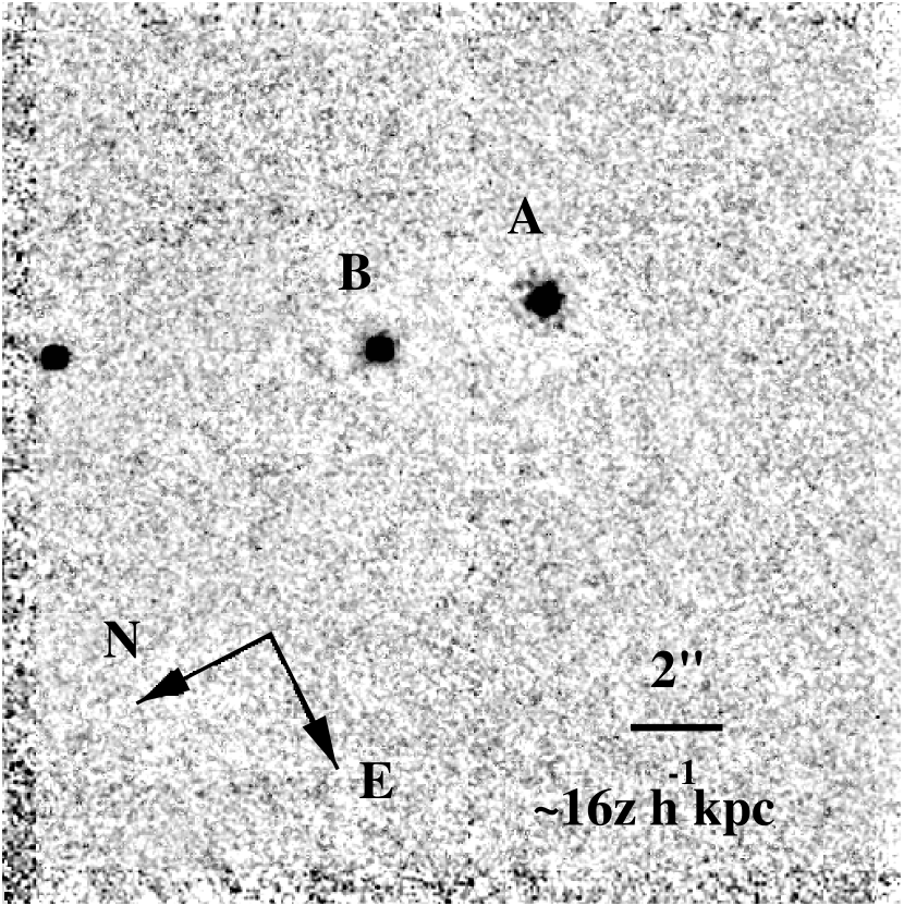
Figure 1: Image of Q 1634+267 A and B. Horizontal bar shown is 2″ in length, which corresponds to roughly 16 $z~{}h_{65}^{-1}\hbox{kpc}$, for an $\Omega=0.1$ open cosmology.

We observed Q 1634+267 on 15 August 1997 with HST using NICMOS Camera 2 (NIC2) and the $H$ (F160W) filter. We obtained four 690-second integrations in a 10.5-pixel dither pattern, for a total integration time of 2560 seconds. We reduced the data with our own software package “nicred” (McLeod 1997; Lehár et al. 1999). Figure 1 shows the reduced, combined image of the field of Q 1634+267. Q 1634+267 A and B are approximately centered in the NIC2 field, and a star is visible at the edge of the $\sim 19\arcsec\times 19\arcsec$ field of view.

2.2 Astrometry and Photometry

The plate scales of the NICMOS cameras changed as the IR array underwent thermal expansion. The variation was monitored (Cox et al. 1998), and the NIC2 plate scales were 0$\farcs$0760926 and 0$\farcs$0754090 per pixel in the X and Y directions, respectively for the measurement nearest the date of observation. The difference in the X and Y plate scales is due to a small tilt of the IR array relative to the focal plane. We adopt a zero point of $M_{H}=21.79\pm 0.02$ for F160W for infinite apertures, based on a comparison of HST archival and ground-based observations of the standard star P330E (Persson et al. 1998). It agrees closely with the value of 21.83 mag obtained by the Space Telescope Science Institute . The foreground Galactic extinction in the direction of Q 1634+267 is only $E(B-V)=0.072$ for $R_{V}=3.1$ (Schlegel, Finkbeiner & Davis 1998); hence, we applied no extinction corrections to our photometric estimates.

We fitted a point-spread function (PSF) to our combined image, to determine the relative coordinates and the magnitudes of Q 1634+267 A and B. Because A and B are well separated, we derived a PSF estimate from both components with the IRAF DAOPHOT package. Table 2 shows the resulting relative coordinates and H-band magnitudes of A, B and the star within our field of view. The quasar images are separated by 3$\farcs$852$\pm$0.003; the brightness ratio A/B is $3.34\pm 0.06$.

We obtained 10-minute snapshots of three quasar pairs, Q 1634+267, Q 1120+0195, and LBQS 1429–008, on 9 Dec 1998 with the VLA in the C array at $\lambda=3.6$ cm. We detected no radio flux to $1\sigma$ limits of $0.028$, $0.030$, and $0.045$ mJy/Beam, respectively. With these low flux limits, there is little hope that further radio observations can shed much light on these systems.

2.3 Magnitude Limit at the Expected Lens Position

Visual inspection of the images revealed no lens candidate near the expected position. To search for a faint lens that might be hidden by A or B, we fitted the PSF derived in the previous section to the quasar components. We then subtracted the fitted PSF from these components. The fainter one, B, was marginally broader than A. The difference might be caused by intrinsic PSF differences at different positions on the detector, and similar small PSF mismatches were seen in other NICMOS archival images containing two or more stars. Thus, we cannot conclude that the slight broadening is due to a faint galaxy underneath quasar B. Such a galaxy would have $m_{H}\gtrsim 21.8$ mag, which is too faint and at the wrong location to be able to produce lensed images with the observed splitting of $\sim 3\farcs 8$.

To determine our detection limit for a lens galaxy, we generated circular galaxies with a de Vaucouleurs profile and an effective radius corresponding to an $L^{*}$ galaxy ($\sim 3h_{65}^{-1}$ kpc) over the redshift range $0.4\lesssim z\lesssim 1.8$ and for $\Omega_{0}=0.1$ and $1.0$ cosmologies. We convolved the redshifted galaxies with the PSF derived from A and B, and added them to our NIC2 frame on a grid of positions within the frame. The resulting images were smoothed with a Gaussian kernel with $\sigma=3$ pixels, and inspected for signs of the added galaxies. We found a magnitude limit of $m_{H}=22.5$ ($1\sigma$) for an early-type lens galaxy. For the sky background in our frame, the standard deviation of the noise level per pixel corresponds to a surface brightness of roughly 23.3 mag arcsec^-2.

3 LOWER LIMIT ON A LENS M/L RATIO

We compute the expected mass to light ratio for a putative lens galaxy for Q 1634+267 from our detection threshold. The anticipated mass of the lens can be derived from simple lens theory assuming it has a singular isothermal sphere (SIS) mass profile. The lens equation relates the angular coordinates $\beta$ ($\theta$) of the source (images), $\vec{\beta}=\vec{\theta}-\vec{\alpha}(\theta)$, where $\alpha(\theta)$ is the deflection angle for an image at $\theta$, with the lens galaxy at the center of coordinates. The SIS assumption implies: $\alpha(\theta)=(1/2)\Delta\theta=4\pi(D_{ds}/D_{s})({\sigma_{v}}^{2}/c^{2})$, where $D_{s}$ ($D_{ds}$) is the distance from the observer (lens) to the source; $\Delta\theta$ is the observed angular separation of the lensed images, and $\sigma_{v}$ is the velocity dispersion of the lens galaxy. Therefore, using the observed image separation one can determine the velocity dispersion $\sigma_{v}$ for a lens galaxy as a function of redshift. We show in Figure 2a the velocity dispersion ${\sigma_{v}}(z)$ using cosmologies $\Omega_{0}=0.1$ and 1, and $H_{0}=65~{}\hbox{km~{}s}^{-1}~{}\hbox{Mpc}^{-1}$. For an A/B magnification ratio of $\mu$, the lens galaxy should lie $\Delta\theta\{\mu/(\mu+1)\}$ from image A along the A-B separation vector.

We translate our magnitude limit of $H=22.5$ into an upper bound on the luminosity of the missing lens galaxy, placed at various redshifts. We follow the method implemented in Keeton et al. (1998) to derive $H$–band luminosity of elliptical galaxies at various redshifts using Charlot & Bruzual (1993) models. The models account for k-correction and passive evolution from formation redshift $z=5$. Coupled with the masses required to produce lensing, determined via the lens equations, the luminosity limits yield the mass-to-light ratio (M/L) as a function of redshift, shown in Figure 2b for cosmologies of $\Omega_{0}=0.1$ and $1$. The most likely (comoving) distance to the lens is half the distance from the observer to the source, where the galaxy has the largest cross section for multiply imaging a source. For Q 1634+267 at redshift 1.961 the most probable lens location is therefore at redshift $0.45$. An elliptical galaxy at $z=0.5$ would have $M/L\gtrsim 1000$ in a low density universe, which is $\gtrsim 50$ times higher than a normal lens galaxy (Keeton et al. 1998, Jackson et al. 1998), and 50 times higher than a limit placed by Turner et al. (1988) in the optical. Therefore, if obscuration is responsible for hiding a lens galaxy with a normal mass to light ratio from view, then the dust must cause at least 4 magnitudes of extinction in the $H$-band. If, however, we accept the Mg ii absorption lines as evidence for a lens galaxy at $z\approx 1.1$ (SS91), then the detection limit of $H>22.5$ corresponds to about $0.15L^{*}_{H}$, or $M/L_{H}\gtrsim 690$ for an E/S0 type galaxy. But if the lens galaxy type is an Sb, at a redshift of $z=1.1$ it would have a $M/L_{H}\gtrsim 430$. The minimum $M/L_{H}$ is $400$ for an Sb galaxy at a redshift of $z=1.3$.

If the lens is an early-type galaxy, we can predict its luminosity from the Faber-Jackson relation (1976) between velocity dispersion $\sigma_{v}$ and luminosity, ${\sigma_{v}/\sigma^{*}}=(L/L^{*})^{1/4}$, where $\sigma^{*}$ and $L^{*}$ are the velocity dispersion and luminosity of an $L^{*}$ galaxy. Studies of lens statistics (e.g. Kochanek 1996) show that the velocity dispersion estimated from the image separation should closely match the central velocity dispersion of the stars. Figure 2a shows the velocity dispersion estimated from the lens geometry as a function of the lens redshift. At $z\approx 0.5$ the predicted velocity dispersion is $\sigma\approx 350~{}\hbox{km~{}s}^{-1}$, considerably higher than the characteristic velocity dispersion of an $L^{*}$ galaxy of $\sigma^{*}\simeq 220\hbox{km~{}s}^{-1}$. A galaxy at $z\approx 0.5$ would be a $L\approx 6L^{*}_{H}$ galaxy, far brighter than normal early-type galaxies, where $1L^{*}_{H}$ would correspond to $H\approx 17.4$ $(16.9)$ mag for a passively evolving stellar population formed at $z_{f}\approx 5$ using the Charlot & Bruzual (1993) models for $\Omega=0.1$ $(1.0)$. Such a bright galaxy would be at least $650$ $(1000)$ times above our detection limit. At the redshift of the Mg ii absorber of $z\approx 1.1$, the required velocity dispersion rises to $\approx 500~{}\hbox{km~{}s}^{-1}$, at the highest end of the range observed for bright galaxies (see for example, Bender et al. 1996). It would have an extreme luminosity of $15L^{*}_{H}$ if the scaling relation continued to hold.

We conclude that the absolute lower limit on the mass-to-light ratio of the putative lens is $M/L_{H}\approx 690$ for an early type galaxy at a redshift $z\approx 1.1$, and $M/L_{H}\gtrsim 400$ for an Sb type at a redshift of $z\approx 1.3$. The limit is higher for any other redshift and for $\Omega_{0}>0.1$. For the most probable lens redshift of $z\approx 0.5$ and the cosmology of a high-density universe, the limit is $M/L_{H}>1000$. Depending on the redshift of the presumed galaxy, the observed $H$ band corresponds roughly to rest $R$ band ($z\approx 1.5$) or $I$ band ($z\approx 0.4$). Since $(B-H)\approx 5.7$ mag for ellipticals at redshift 0.5, and $(B-H)_{\odot}=1.91$ mag, the limit would be about 30 times higher for $M/L_{B}$ than for $M/L_{H}$. If Q 1634+267A,B is the split image of a single quasar, the lens must be a galaxy with an unprecedentedly high mass-to-light ratio.

In fact, as we discuss in §4, there are no galaxies above a detection limit of $\approx 0.1L^{*}_{H}$ within $40h_{65}^{-1}$ kpc and no galaxies above a detection limit of $\approx 1L^{*}_{I}$ within $100h_{65}^{-1}$ kpc of the quasars. Thus the depth of the imaging also rules out any normal cluster of galaxies centered near the expected lens position. Moreover, the limit on the optical $M/L$ of $M/L_{B}\approx 10^{4}h_{65}$ greatly exceeds even the usual estimates for groups and clusters of galaxies, where virial $M/L\approx 200$–$400h$ (e.g., see Carlberg et al. 1996, Bahcall et al. 1995, David et al. 1995) is typical.

4 THE NATURE OF THE Mg ii ABSORBER

In Q 1634+267A,B, metal absorption lines are observed at $z=1.839$ and $z=1.126$ (Sargent & Steidel (1991), Djorgovski & Spinrad (1984), and Turner et al. (1988)). Mg ii $\lambda\lambda 2796,2803$ absorption doublets with equivalent widths like the EW₀(Mg ii $\lambda 2796)=1.51$Å doublet at $z=1.126$ (SS91) are associated with chemically enriched material in the halos of visible, luminous galaxies along the line of sight (e.g. Steidel 1993, 1995; Steidel et al. 1997). Because quasars show roughly one metal line absorption system per unit redshift down to a typical rest equivalent width limit of $\sim 0.3$Å (e.g. Steidel 1993), the mere presence of a metal absorption system is not evidence for the presence of a lens galaxy. In a survey of galaxies selected by the presence of Mg ii absorption, Steidel (1993) showed that the absorbers are associated with galaxies of Hubble types from E to Sb. The strength of the absorption is anti-correlated with the distance of the quasar from the nearest luminous galaxy, and it is correlated with the intrinsic brightness of the galaxy (Steidel 1995, 1993). The luminosities of the $\sim 70$ systems studied by Steidel (1995) and Steidel et al. (1997) range from $0.02L^{*}$ to $4L^{*}$ with 90% (61/70) having $L>0.1L^{*}$. All but one (i.e. 99%) of the galaxies were found within a projected radius of $40h_{65}^{-1}$ kpc.

We searched both the NICMOS H image and existing HST WFPC1 optical images (obtained under GTO-1116 by Westphal) for signs of a galaxy associated with the $z=1.126$ absorption feature. Since the absorbing galaxy could have an exponential disk profile rather than the de Vaucouleurs profile considered in §2, we re-derived the detection limit for an exponential disk galaxy with a scale factor of $4\ h^{-1}_{65}$ kpc. The limit of $22.5$ mag ($1\sigma$ for $\Omega_{0}=0.1$) was similar to that for a de Vaucouleurs model with a $3\ h^{-1}_{65}$ kpc effective radius. In the evolutionary models of Charlot & Bruzual (1993), a passively evolving $L^{*}$, Sb-type, galaxy which formed at $z_{f}=5$ would have $H_{*}\approx 19.7$ for $\Omega_{0}=1.0$, and $H_{*}\approx 20.0$ for $\Omega_{0}=0.1$, at $z=1.126$. Therefore, our detection limit implies that we could have detected a galaxy with $L>0.1L^{*}_{H}$ anywhere within an impact parameter at $40h_{65}^{-1}$ kpc from Q 1634+267A (to the edge of the NICMOS array along the short direction). We derive a weaker detection limit of $L>L^{*}_{I}$ from the F785LP (I-band) out to $100h_{65}^{-1}$ kpc. Thus, any galaxy associated with the $z=1.126$ Mg ii absorption feature is either unusually faint or distant compared to those found in the Steidel (1993, 1995) surveys.

Since the PSF of quasar B is broader than that of quasar A, it is unlikely that the null detection could be explained by a galaxy directly under Q 1634+267A, although we cannot exclude a very sub-luminous, compact dwarf with perfect alignment. Alternatively, a galaxy with a luminosity $\gtrsim$ $1L^{*}_{B}$ lying outside our field of view might be responsible for the absorption. Distant ($>40\ h^{-1}_{65}$ kpc), luminous ($L>L^{*}$) galaxies are associated with absorption, but the Mg ii equivalent widths are less than 0.4Å (Steidel 1995, Steidel et al. 1997), compared to the observed 1.5Å. For distant absorbers it is also odd that no equivalent Mg ii absorption feature is seen in Q 1634+267B. In summary, the absorbing galaxy falls outside of the parameter space populated by galaxies found in Mg ii absorber survey. The absorber must therefore be very under-luminous, $\lesssim 0.1L^{*}_{H}$.

5 SIMILARITY OF THE QUASAR SPECTRA

In the absence of a lens galaxy, it is the remarkable spectral similarity of many of the quasar pairs which provides the impetus for the gravitational lens interpretation. The spectra of the Q 1634+267A,B pair show some of the greatest similarities of the pair population, and Small et al. (1997) have demonstrated that the observed differences are consistent with the temporal variations of quasar spectra over epochs separated by months to years. No study, however, has examined whether the spectra of the close pairs show a degree of spectral similarity that is statistically greater than that of randomly selected quasars. An affirmative answer increases the credibility of the lens hypothesis, because the lens hypothesis provides a natural explanation for the spectral similarities. While it would not rule out the binary hypothesis, it leaves a serious puzzle as to why the nuclear regions of two separate galaxies have such highly correlated emission properties. We start by defining how we will measure spectral similarities, and then estimate the likelihood of finding a single quasar pair with spectra as similar as Q 1634+267A,B. In isolation, the significance is hard to interpret because we picked Q 1634+267A,B for study due to its spectral similarities. Thus, in our final step we estimate the likelihood of finding a population of quasar pairs with the observed spectral similarities.

5.1 Sample Definition

We will compare spectra using the observed differences between the spectral slope $\alpha$ and the rest equivalent widths (EW₀) of the Ly $\alpha$, C iv ($\lambda\lambda$1548, 1550) and C iii] ($\lambda$1909) emission lines. We selected these features because they are commonly measured in statistical surveys of quasar spectra. For Q 1634+267 we computed the indices from the SS91 spectra. These calibrated spectra were taken at the Palomar 5-meter, using a double spectrograph that covered the blue (3150–4750Å) and the red (4600–7000Å) wavelengths. We used either the Large Bright Quasar Survey (LBQS) or the pair population as a whole for a comparison sample.

The LBQS consists of 1055 optically selected quasars (Foltz et al. 1987, Foltz et al. 1989, Hewett et al. 1991). We use the measurements of the spectral indices for the LBQS quasars from Francis (1996), Hewett et al. (1995), Francis (1993a), and Francis et al. (1991). The binned distributions for the LBQS quasars were fitted with analytic functions (composites of Gaussians and Lorentzians) to provide smooth probability distributions. Some of the spectral features are correlated (Francis et al. 1992; Francis 1993a), and we will conduct tests to examine the effects of these correlations on the probability calculations.

Unfortunately we lack a complete spectral database for the pairs, although the uncanny similarity of Q 1634+267A,B is not an isolated case. There are 14 quasar pairs with angular separations $3\arcsec\lesssim\theta\lesssim 10\arcsec$ and similar redshifts (see Table 1). We will frequently refer to this as our 14 pair sample. Of these 14, we can reject 7 as lenses. In the cases of PKS 1145–071, HS 1216+5032, Q 1343+2640, J 1643+3156 and MGC 2214+3550, only one of the quasars is a radio source; in the case of Q 0151+048 the small emission line redshift difference is confirmed by an absorption feature in the background quasar; in LBQS 2153–2056, the spectrum of quasar B shows a strong absorption blueward of the C iv emission line. Four of these binaries (QJ 0240–343, PKS 1141–071, HS 1216+5032, Q 0151+048) show fairly similar spectra, although they all have at least one significant spectral difference. Of the 7 ambiguous pairs, five (Q 2138–431 in Hawkins et al. 1997, Q 1429–008 in Hewett et al. 1989, Q 1634+267 and Q 2345+007 in SS91, Q 1120+0195 in Michalitsianos et al. 1997) show remarkably similar optical spectra. For the pair sample we restrict our comparison to the C iv equivalent width and the power law slope $\alpha$ because the other two indices are not consistently observed or are impossible to measure without the original data.

5.1.1 Line and Continuum Slope Measurements

To determine the spectral slope, we fit a power law (defined as F${}_{\nu}\propto\nu^{\alpha}$) excluding regions where there are emission or absorption lines. The Fe ii in the UV spectra of quasars introduce substantial uncertainty in the measurement of continuum slopes. The power law $\alpha$ is also uncertain in the blue spectrum from contamination due to the extended wings of the C iv, N v, and Ly $\alpha$ emission lines, as well as the Ly $\alpha$ forest absorption. Because of these complications, the width of the spectral slope distribution remains controversial. Some (e.g. Elvis et al. 1994; Webster et al. 1995) find large dispersions, while others find little or no dispersion in $\alpha$ (Francis 1996; Sanders et al. 1989). In our analysis we will adopt the narrow $\alpha$ distribution from Francis (1996), as derived from 30 LBQS quasars. The Francis (1996) distribution has a root-mean-squared (RMS) width of $\sigma_{\alpha}=0.3$, compared to $\sigma_{\alpha}=0.5$ for the broader distributions of Francis et al. (1992). In Q 1634+267 the mean slopes are $\alpha=-0.17$ in the blue (observed 3150–4734Å) and $\alpha=-0.12$ in the red (observed 4580–6985Å) spectra respectively. In both the blue and the red, the power law indices between A and B differ by $\Delta\alpha=0.03\pm 0.03$.

When comparing equivalent widths we must be careful to use identical measurement methods because of the difficulties introduced by line blending and continuum definition. Francis (1993a) showed that C iv equivalent widths can vary by a factor of two depending on the measurement method, and thus broaden the distribution of equivalent widths by the same factor. For Q 1634+267A,B we avoid these problems by using the same definitions followed by the LBQS (Francis 1993a). For this method, continuum windows are defined on both sides of a given line. Then the flux is summed above a line adjoining the continuum windows, over a region known as the line window. The continuum windows are chosen to exclude the flux contributed by nearby broad lines, so the line fluxes should be considered a lower limit. The difference in rest equivalent widths (EW₀) between A and B are 3Å for C iv, 8Å for Ly $\alpha$ and 3Å for C iii]. Measuring EW₀(C iv) requires connecting the red and blue halves of the spectra because the blue side spectrum terminates on the red wing of the C iv emission line, causing the continuum windows to fall on different spectrographs. We calculate a scaling factor of 1.22 using the regions of overlap. But there is some evidence that the same scaling factor might not apply to quasar B because of large fluctuations in the data over that region. Therefore the EW₀(C iv) differences of 3Å should be considered an upper limit. Indeed, restricting ourselves to the blue regions alone and fitting Gaussians to the emission lines we find quasars A and B to differ at most by $\Delta$EW₀(C iv)$~{}=1$Å. The two methods yield the same flux. For completeness, and because the numbers have not been published elsewhere, we also measure other line fluxes and summarize them in Table 2, although some we do not use in our analysis. All of the line fluxes are measured with the technique described in Francis (1993a) except for N v. Because the blending with Ly $\alpha$, the measurement for N v lines is done by fitting Gaussians to Ly $\alpha$ simultaneously with N v where we assumed that both lines are similar in shape.

For the other quasar pairs we estimated bounds on the C iv equivalent width and the spectral index $\alpha$ based on the published spectra. For the 5 most similar pairs, we estimate that they have spectral differences $\Delta\alpha\lesssim 0.1$ and $\Delta$EW₀(C iv) $\lesssim 6$Å (see Table 3). For the two pairs whose spectra have the worst noise (Q 1120+0195 (Michalitsianos et al. 1997) and Q 1429–008 (Hewett et al. 1989)) the estimates are rough, while they are more accurate for the other three pairs. Since the estimates of the equivalent widths may be imprecise, we will also quote results by doubling our bound on the differences to $\Delta$EW₀(C iv) $\lesssim 12$Å. We summarize our parameter estimates for the pairs in Table 3.

5.1.2 Joint Probabilities and Correlations among Spectral Features

To compute the probability that two random quasars have given differences in C iii], Ly $\alpha$, C iv equivalent widths and spectral slope $\alpha$, we randomly draw the properties of two quasars at a time from the compiled number distributions. If the spectral features are completely uncorrelated, the likelihood that two quasars are similar to each other, i.e. have differences of less than $\Delta$EW₀(C iv), $\Delta$EW₀(C iii]), etc., is simply the joint product of each individual probability. However, if there are correlations, they could make the alarming similarities of the quasar pairs a trivial selection effect. Therefore we first explore the extent to which spectral features are correlated.

Through a principal component analysis, Francis et al. (1992) showed that the equivalent widths of quasar emission lines are correlated with the power law slope $\alpha$. Francis (1993b) further showed that $\alpha$ is correlated with redshift. Their study was based on correlations with a spectral slope distribution in Francis et al. (1992) which has a large RMS dispersion of about $\sigma_{\alpha}=0.5$. The strongest correlation, Al iii$+$C iii] with $\alpha$, has a large scatter; the correlations of this and other lines are very weak. Subsequently, Francis (1996), using more accurate photometry, found that the spectral slope distribution actually has a much narrower dispersion of $\sigma_{\alpha}=0.3$. But the newer study does not affect the dispersions of the line strengths, which are more accurate as long as they are measured consistently. Because the scatter of the line strengths remains large for a much reduced range in spectral slopes, the correlations are weaker in light of the narrow distribution compared to Francis et al. (1992). Furthermore, plotting spectral slope vs. redshift from Francis (1996) shows that there is no correlation between the two parameters. In the analysis below, we will use the narrow power law distribution found in Francis (1996). Therefore, the correlations between line emission, continuum, slopes and redshifts can be safely ignored for our purposes.

Nonetheless, to confirm that correlations are unimportant even under extreme scenarios we conduct the following Monte Carlo experiment to choose quasars from the number distributions found in Francis et al. (1992) and Francis (1993a). We select from the broader spectral slope distribution where correlations were originally found. The correlation between emission line strengths and $\alpha$, and $\alpha$ with redshift $z$, means that the process of drawing quasars must proceed in a sequence to account for correlations at each step: first we draw quasars out of the LBQS redshift distribution, then the spectral slope distribution, followed at last by the emission line distribution. To account for the correlation of $\alpha$ with redshift we do the following. Having picked a redshift, and given the power law distribution $\alpha$, we offset the entire distribution by an amount $d\alpha=0.79\times d~{}log(1+z)$ (See Figure 2 of Francis 1993b). We can then randomly select a value of $\alpha$ from this new distribution. There is, however, one subtlety. The distribution for $\alpha$ contains no redshift information because it is summed over all redshifts. But because of the correlation, if quasars at any given redshift have a small dispersion in their spectral slopes, as one accumulates the distribution over broader redshift ranges, the net distribution would also gradually become wider. We account for this effect by arbitrarily shrinking the dispersion and then drawing from this narrower spectral slope distribution instead of the original, broader one. We verified that decreasing the dispersion by 25%, more than one would expect, would not significantly alter our discussions below. Once a value for $\alpha$ has been selected, one can then proceed in the same fashion to select from the number distribution of C iii], C iv, or Ly $\alpha$, accounting for their roughly linear correlations with $\alpha$ by: $EW_{line}=m\alpha+b$ where the correlation coefficients $m$ and $b$ are given in Francis et al. (1992). Again, we verified that any correlations would only begin to affect our conclusions if the number distributions were all narrowed by more than 25%.

There may also be weak correlations of quasar spectral properties with luminosity. The pair members share a common redshift and have similar luminosities, so we would under-estimate the likelihood of the members possessing similar spectra if the distributions of spectral indices are correlated with either variable. We saw that the spectral index correlation with redshift has little or no role in our analysis. The Baldwin (Baldwin 1977) effect, a correlation between luminosity and C iv equivalent width, has been studied extensively (e.g. more recently see Kinney et al. 1990, Sargent et al. 1989, Baldwin et al. 1989). Their results show that at a given luminosity the equivalent widths of the C iv emission line have a defined range in strengths, with a scatter of about 20Å. The strength of the C iv lines decreases with luminosity and the relation holds over 7 orders of magnitude in quasar luminosity. The parameterization of the correlation: $EW({\sc C~{}iv})\propto L^{\beta}_{1450}$ has $\beta$ ranging from $\beta=-0.07$ (Francis et al. 1992) to $\beta=-0.45$ (Smetanka et al. 1991). LBQS quasars, being a magnitude limited sample, have only a small spread in absolute luminosity, $-28\lesssim M_{B}\lesssim-26$ (Francis et al. 1992). Since at any luminosity there is a considerable scatter in C iv and vice versa (see Osmer & Shields 1988 for summary), we do not expect the luminosity correlations to affect our analysis. Nonetheless, we tested for any effects by deriving the distribution of $\Delta\hbox{EW}_{0}({\sc C~{}iv})$ both with and without limits on the luminosity difference $\Delta L$ of the quasars making up the simulated pairs using the $B_{J}$ magnitudes and EW₀(C iv) values for the 439 LBQS survey quasars from Francis (1993). We found no significant differences between the distributions without a luminosity restriction and those where the quasars were required to have absolute luminosities differing by less than a factor of 5 ($1.7$ mag) or a factor of 2.5 ($1$ mag).

Because the parameter correlations are very weak, in the discussions that follow, we make the assumption that no two spectral features are correlated.

5.2 The Spectral Similarity of Q 1634+267A,B

As discussed previously, the spectra of Q 1634+267 A and B have equivalent width differences $\Delta\leq 3$Å for ${\sc C~{}iv}$; 8Å for Ly $\alpha$; and 3Å for C iii], as well as 0.03 for $\alpha$. If we select randomly from the distributions of these features in the LBQS survey, the probability of finding two quasars with smaller differences are 11%, 16%, 30%, and 12% respectively. Assuming no correlations between the features, the joint probability of the differences being as small as observed is 0.06%.

With such a low joint probability, it would be reasonable to find several quasars with such similar spectra in the total quasar population ($\sim 10^{4}$ quasars), but highly unlikely to find any in the tiny sub-population of quasar pairs ($14$ objects). The strength of this conclusion depends only weakly on the details of the comparison, and the joint probability only rises to 1% if we confine the comparison to the spectral index and C iv equivalent width differences. Adding additional spectral features to the estimate would further reduce the likelihood, but it becomes increasingly important to fully understand the spectral correlations of quasars. Moreover, calculations of a posteriori probabilities can generally yield arbitrarily low likelihoods by over-specifying the problem. Nonetheless, the similarity of the Q 1634+267 A and B spectra extends across the entire rest-UV spectra of the pair.

5.3 The Spectral Similarity of the Pair Population

Because we pre-selected Q 1634+267A,B for study because of its spectral similarities, we cannot interpret it in isolation from the rest of the pair population. Moreover, the uncanny similarities of Q 1634+267A,B are not an isolated example among the pairs. To fully understand the significance of the spectral similarities of the pairs, we must consider the entire pair population.

Under the assumption that the quasars making up the pair sample are drawn from the same parent population as the quasars in the LBQS, we can produce mock samples of quasar pairs by randomly selecting 14 pairs of quasars from the LBQS. We can then compare the distribution of the spectral slope and C iv equivalent width differences, $\Delta\alpha$ and $\Delta$EW₀(C iv), to those observed for the pairs. We will estimate the probability of finding at least as many similar pairs as observed in the real sample.

We generated $10^{4}$ mock pair catalogs to determine the fraction of catalogs in which N_sim pairs have spectral differences smaller than the specified limits on $\Delta\alpha$ and $\Delta$EW₀(C iv), with the results illustrated in Figure 3. The top panel shows the limits on spectral similarity ($\Delta\alpha\lesssim 0.1$ and $\Delta$EW₀(C iv)$\lesssim 6$Å) which characterize the differences observed for the 5 pairs with similar spectra (Q 2138–431, LBQS 1429–008, Q 1634+267, Q 1120+0195 and Q 2345+007). The chance of drawing 5 or more pairs with such similar spectra in the sample of 14 pairs is about 0.2%. If we were to relax the constraints to $\Delta\alpha\lesssim 0.1$ and $\Delta$EW₀(C iv)$\lesssim 12$Å to account for possible systematic errors in measuring $\Delta$EW₀(C iv), the probability for finding 5 or more such pairs grows only to 3%. We conclude that the likelihood for finding 5 pairs with such similar spectra in a sample of 14 pairs is low. If we significantly broaden the criterion for similarity ($\Delta\alpha\lesssim 0.2$ and $\Delta$EW₀(C iv)$\lesssim 20$Å), the likelihood of finding five or more similar pairs rises to 60%. However, with these weaker criteria there are now seven observed pairs meeting the criterion for similarity (we should add QJ 0240–343 and LBQS 2153–2056), and the likelihood of finding seven or more similar pairs is then smaller, at 20%. We regard this third case as a significant under-estimate of the similarities. The low probability for finding similar quasars randomly, using two parameters, may only be an upper bound. If our pairs sample were partly made up of gravitational lenses, microlensing and time delay might cause some spectral differences in those systems. It is impossible to quantify such a conjecture with our pairs sample.

The probability for finding similar quasars is significantly lower if we use a broad continuum slope distribution (e.g. Francis 1992) rather than the narrow distribution of Francis (1996) used for the estimates in Figure 3. For the broad estimate of the $\alpha$ distribution, the likelihoods for drawing at least 5 similar pairs under the same three sets of constraints on $\Delta\alpha$ and $\Delta$EW₀(C iv) are 0.01, 0.2% and 1.2% instead of 0.2%, 3.0% and 20% (see Figure 4). Thus, the debate about the width of the continuum slope distribution does not alter the conclusion that the spectral similarities of the pairs are unlikely to occur by chance unless the distribution is even narrower than that found by Francis (1996). The distribution of C iv equivalent widths, as long as measured consistently, does not suffer from the systematic problems of the spectral slope distribution.

6 CONCLUSIONS

We again confirm that there is no sign of a lensing galaxy or a surrounding group or cluster of galaxies near the Q 1634+267A,B quasar pair. Our limit on the mass-to-light ratio is $\gtrsim 690h_{65}$ in the $H$ band, tighter than previous estimates. We also lack a candidate galaxy within $100h_{65}^{-1}$ kpc for producing the $z=1.126$ Mg ii absorption feature in the spectrum of A. Since the existence of even one large separation lens produced by a “dark” mass distribution has profound implications, confirming or disproving the lens hypothesis is highly desirable. It appears from the data in the literature that the flux ratio of the quasars is significantly time variable, changing from 4.4 (Djorgovski & Spinrad 1984) to 2.83 (Turner et al. 1988), to 3.28 (SS91) and 3.34 (this work). With its large angular separation, regular photometric monitoring of the system to search for a time delay would be simple on modest size, ground-based telescopes. Although we found that the pairs Q 1634+267, Q 1120+0195, and LBQS 1429–008, are at best weak radio sources, with upper limits on their fluxes of $0.28$, $0.030$, and $0.045$ mJy/Beam at $\lambda=3.6$ cm, deeper observations may still detect the sources or demonstrate that both members are at the extremes of the radio to optical flux ratio distribution. Deep X-ray observations would also be useful, both to measure the flux ratio of the quasars and to search for hot X-ray emitting gas associated with any lensing potential. Deep IR imaging should detect the quasar host galaxies, whose shapes must show tangential, arc distortions under the lens hypothesis.

The spectral similarities of some of the quasar pairs has always been the major impetus for the “dark” lens interpretation of the systems. To date, these arguments have been based on the similarities of individual pairs rather than the overall pair population. Using the distribution of continuum slopes and C iv equivalent widths, we demonstrated that it was improbable to find as many similar pairs as observed in the existing sample of 14 pairs. The probability estimates range from 0.01% to 3%, depending on how strictly similarity is defined and depending on whether a broad or narrow distribution was used for the continuum slope distribution. A better quantitative analysis needs a uniform spectral survey of the pairs.

The effects of binary quasar interaction on spectral similarity have been surmised, for example, by Schneider (1993). Kochanek et al. (1999) demonstrated that most of the quasar pairs are binary quasars rather than “dark lenses.” The binary quasar hypothesis is a successful quantitative interpretation of both the number of quasar pairs and the distribution of their separations. If they are all binary quasars, then there must be a physical explanation for the spectral similarities. Binary quasars are examples of quasar activity triggered by mergers, which represent a small fraction of all quasar activity (about 5% in simple models, see Kochanek et al. 1999a). We present two hypotheses for how binary quasars can have such similar spectra. First, if the physical properties of quasars triggered by major mergers (e.g. mass, accretion rate, surrounding gas density) were confined to a limited range of values compared to the overall quasar population, then the observable properties of the binaries would be more similar than those of randomly selected quasars. This hypothesis has a definite, testable prediction – the spectra of the different pairs should be more similar to each other than for randomly selected quasars. It would also be expected that the quasar host galaxies have properties commensurate with being the products of major mergers – which can be tested by deep imaging. Second, if quasar spectra have a significant dependence on the age of the activity, then the binary spectra are more similar than for random quasars because the merger provides a common triggering event for the activity in the two systems. Here we would not expect the spectra of the different pairs to show any more similarity than randomly selected quasars. In either case, the binary quasar population becomes a very important probe of the physics of quasars because it provides evidence for correlations between events on large scales and the detailed operation of the central engine.

7 ACKNOWLEDGMENTS

We are very grateful to C.C. Steidel for providing the Q 1634+267 spectrum used in our analysis and to P.J. Francis for supplying the luminosity and C iv data for the LBQS quasars. We also thank C.B. Foltz, L.C. Ho, A.V. Filippenko, W.D. Li, A. Quillen, and G. Rudnick for enlightening discussions, and the referee P. Schneider for his comments. Support for the CASTLES project was provided by NASA through grant numbers GO-7495 and GO-7887 from the Space Telescope Science Institute, which is operated by the Association of Universities for Research in Astronomy, Inc. CSK and CRK were also supported by the NASA Astrophysics Theory Program grant NAG5-4062. HWR is also supported by Fellowship from the Alfred P. Sloan Foundation. Our research was supported by the Smithsonian Institution.

Table 1: Quasar Pairs With Separations of 3″ to 10″

Name	$z_{s}$	$\Delta\theta$	$R$	$f_{O}$	$f_{R}$	$F_{20}$	$|\Delta v|$	Lens?	Type	Ref
			$h_{50}^{-1}$ kpc			mJy	km s-1
Q 0151+048†	$1.91$	$3\farcs 3$	$28$	27.5		$<1$	$520\pm 160$	No	$O^{2}$	1
PKS 1145–071	$1.35$	$4\farcs 2$	$36$	2.1	$>500$	$740$	$200\pm 110$	No	$O^{2}R$	2
HS 1216+5032	$1.45$	$9\farcs 1$	$78$	5.2	$>28$	$3.9$	$260\pm 1000$	No	$O^{2}R$	3
Q 1343+2640	$2.03$	$9\farcs 5$	$78$	1.1	$>57$	$8.6$	$120\pm 890$	No	$O^{2}R$	4
J 1643+3156	$0.59$	$2\farcs 3$	$17$	1.3	$>40$	$120$	$80\pm 10$	No	$O^{2}R$	5
LBQS 2153–2056	$1.85$	$7\farcs 8$	$64$	14.5		$<1$	$1100\pm 1500$	No	$O^{2}$	6
MGC 2214+3550	$0.88$	$3\farcs 0$	$26$	1.6	$>42$	$246$	$148\pm 420$	No	$O^{2}R$	7
MG 0023+171	$0.95$	$4\farcs 8$	$40$	3.0	$\sim 10$	$186$	$292\pm 260$	?–	$O^{2}R^{2}$	8
Q 1120+0195††	$1.46$	$6\farcs 5$	$56$	173.8		$<1$	$628\pm 120$	?–	$O^{2}$	9
LBQS 1429–008	$2.08$	$5\farcs 1$	$42$	17.4		$<1$	$260\pm 300$	?–	$O^{2}$	10
QJ 0240–343	$1.41$	$6\farcs 1$	$52$	2.1		$<1$	$250\pm 180$	?	$O^{2}$	11
Q 1634+267	$1.96$	$3\farcs 8$	$32$	4.4		$<1$	$33\pm 86$	?	$O^{2}$	12
Q 2138–431	$1.64$	$4\farcs 5$	$38$	3.0			$0\pm 115$	?	$O^{2}$	13
Q 2345+007	$2.15$	$7\farcs 3$	$58$	4.0	$>9$	$0.035$	$476\pm 500$	?	$O^{2}$	14
RXJ 0911.4+0551	$2.80$	$3\farcs 1$	$24$	1.9		$<1$	$158\pm 1000$	Yes	$O^{2}$	15
Q 0957+561	$1.41$	$6\farcs 1$	$52$	1.4	$1.3$	$552$	$200\pm 15$	Yes	$O^{2}R^{2}$	16
HE 1104–1805	$2.32$	$3\farcs 1$	$24$	4.8		$<1$	$300\pm 90$	Yes	$O^{2}$	17
MG 2016+112	$3.27$	$3\farcs 6$	$26$	1.7	$\sim 1$	$191$	$40\pm 100$	Yes	$O^{2}R^{2}$	18

Note. — $z_{s}$ is the source redshift, $\Delta\theta$ is the angular separation, $R$ is the projected separation at the source redshift for $\Omega_{0}=1$ and $H_{0}=50h_{50}$ km s^-1 Mpc^-1, $f_{0}$ and $f_{R}$ are the optical and radio flux ratios or their lower limits, $F_{\lambda}$ is the radio flux of the brighter image at wavelength $\lambda$ (in cm), and $|\Delta v|$ is the velocity difference between the quasars. The entries in the Lens? column are: “Yes” if a normal lens (galaxy, group, or cluster) is seen in the correct position to produce the observed system, there is no significant velocity difference, and the radio and optical data are consistent with the lens hypothesis; “No” if we see no lens and either the radio emission or the emission line velocity difference, confirmed by an absorption line velocity difference, are inconsistent with the lens hypothesis; and, “?” if we see no lensing object but have no objective criterion to decide whether or not the object is lensed. If there is some evidence that the system is actually a binary, we used the label “?–”. Type denotes the optical/radio classification of the pair. Note that MG 2016+112 is really a triple system, not a pair.

^†Q 0151+048 is also named PHL 1222 and UM 144.

^††Q 1120+019 is also named UM 425.

References: (1) Meylan et al. 1990, (2) Djorgovski et al. 1987, (3) Hagen et al. 1996, (4) Crampton et al. 1988, (5) Brotherton et al. 1999, (6) Hewett et al. 1997, (7) Muñoz et al. 1997, (8) Hewitt et al. 1987, (9) Meylan & Djorgovski 1989, (10) Hewett et al. 1989, (11) Tinney 1995, (12) Djorgovski & Spinrad 1984, (13) Hawkins et al. 1997, (14) Weedman et al. 1982, (15) Bade et al. 1997, (16) Walsh et al. 1979, (17) Wisotzki et al. 1993, (18) Lawrence et al. 1984.

Table 2: Observed Properties of Q 1634+267 A,B

Parameter	Value
Image separation	$3\farcs 852\pm 0.003$
$\Delta$ RA	$-0\farcs 673$
$\Delta$ DEC	$3\farcs 793$
H-magnitude of component A	$18.26\pm 0.01$
H-magnitude of component B	$19.56\pm 0.01$
H-magnitude of star	$19.67\pm 0.01$
Flux ratio (A/B)	$3.34\pm 0.06$
Power law slope $\alpha$	$-0.13$
EW0(Ly $\alpha$)	$47.95$Å
EW0(N v $\lambda$1240)	$24.18$Å
EW0(Si iv $\lambda$1400)	$11.83$Å
EW0(C iv $\lambda\lambda$1548, 1550)	$37.44$Å
EW0(C iii] $\lambda$1909)	$16.91$Å

Table 3: QSOs A,B Parameter Difference Estimates

	$\Delta\alpha$	$\Delta$EW0(C iv) Å	Lens?	References
Q 1120+0195	0.1	6	?	Michalitsianos et al. 1997
LBQS 1429–0053	0.03	6	?	Hewett et al. 1989
Q 1634+267	0.03	3	?	Steidel & Sargent 1991
Q 2138–431	0.02	6	?	Hawkins et al. 1997
Q 2345+007	0.07	3	?	Steidel & Sargent 1991
LBQS 2153–2056	0.05	14	No	Hewett et al. 1998
QJ 240–343	0.2	20	No	Tinney 1995

Note. — Estimated differences between the spectra of QSO pairs A and B from published spectra in literature.

Figure 2: (a) Anticipated velocity dispersion of a putative lens galaxy and (b) $M/L_{H}$ ratio as function of redshift for a putative lens galaxy, assuming properties of an early-type galaxy.

Figure 3: The fraction of trials in which $N_{sim}$ pairs from a sample of 14 pairs randomly drawn from the LBQS meet the stated conditions on $\Delta\alpha$ and $\Delta$EW₀(C iv). We assume the narrow spectral slope distribution from Francis (1996). The arrow marks the number of pairs observed to meet the similarity condition. (a) Representative spectral differences actually observed for the five lens candidates. Probabilities for (b) and (c) have substantially weaker C iv and spectral slope constraints, as indicated in each box.

Figure 4: The fraction of trials in which $N_{sim}$ pairs from a sample of 14 pairs randomly drawn from the LBQS meet the stated conditions on $\Delta\alpha$ and $\Delta$EW₀(C iv). Here we assume the broad spectral slope distribution from Francis et al. (1992). The arrow marks the number of pairs observed to meet the similarity condition. The cases similarity conditions are the same as in Figure 3.

References

- (1)
- (2) Bade, N., Siebert, J., Lopez, S., Voges, W., Reimers, D., et al. 1997, A&A, 317, 13
- (3)
- (4) Bahcall, N. A., Lubin, L. M., & Dorman, V. 1995, ApJ, 447, L81
- (5)
- (6) Baldwin, J. A. 1977, ApJ, 214, 679
- (7)
- (8) Baldwin, J. A., Wampler, E. J., & Gaskell, C. M. 1989, ApJ, 338, 630
- (9)
- (10) Bender, R., Ziegler, B., Bruzual, G. 1996, ApJ, L51
- (11)
- (12) Brotherton, M. S., Gregg, M. D., Becker, R. H., Laurent-Muehleisen, S. A., et al. 1999, ApJ, 514, L61
- (13)
- (14) Carlberg, R. G., Yee, H. K. C., Ellingson, E., Abraham, R., et al. 1996, ApJ, 462, 32
- (15)
- (16) Charlot, S. & Bruzual, A. G. 1993, ApJ, 405, 538
- (17)
- (18) Cox, C. et al. 1997, Instrument Science Report, OSG-CAL-97-07, Space Telescope Science Institute
- (19)
- (20) Crampton, D., Cowley, A. P., Hickson, P., Kindl, E., et al. 1988, ApJ, 330, 184
- (21)
- (22) David, L. P., Jones, C., & Forman, W. 1995, ApJ, 445, 578
- (23)
- (24) Djorgovski, S., & Spinrad, H. 1984, ApJ, 282, L1
- (25)
- (26) Djorgovski, S., Perley, R., Meylan, G., & McCarthy, P. 1987, ApJ, 321, L17
- (27)
- (28) Elvis M., Wilkes, B. J., McDowell, J. C., Green, R. F., et al. 1994, ApJS, 95, 1
- (29)
- (30) Faber, S. M. & Jackson, R. E. 1976, ApJ, 204, 668
- (31)
- (32) Filippenko, A. V. 1989, ApJ, 338, L49
- (33)
- (34) Fisher, K. B., Bahcall, J. N., Kirhakos, S., & Schneider, D. P. 1996, ApJ, 468, 469
- (35)
- (36) Foltz, C. B., Chaffee, F. H. Jr., Hewett, P. C., MacAlpine, G. M., et al. 1987, AJ, 94, 1423
- (37)
- (38) Foltz, C. B., Chaffee, F. H. Jr., Hewett, P. C., Weymann, R. J., et. al 1989, AJ, 98, 1959
- (39)
- (40) Francis, P. J., Hewett, P. C., Foltz, C. B., Chaffee, F. H., et al. 1991, ApJ, 373, 465
- (41)
- (42) Francis, P. J., Hewett, P. C., Foltz, C. B., & Chaffee, F. H. 1992, ApJ, 398, 476
- (43)
- (44) Francis, P. J. 1993a, ApJ, 405, 119
- (45)
- (46) Francis, P. J. 1993b, ApJ, 407, 519
- (47)
- (48) Francis, P. J. 1996, Publ. Astron. Soc. Aust., 13, 212
- (49)
- (50) French, H. B., & Gunn, J. E. 1983, ApJ, 269, 29
- (51)
- (52) Jackson, N., Helbig, P., Browne, I., Fassnacht, C. D., et al. 1998, A&A, 334, L33
- (53)
- (54) Hagen, H.-J., Hopp, U., Engels, D., & Reimers, D. 1996, A&A, 308, L25
- (55)
- (56) Hawkins, M. R. S., Clements, D., Fried, J. W., Heavens, A. F., et al. 1997, MNRAS, 291, 811
- (57)
- (58) Hewett, P. C., Webster, R. L., Harding, M. E., Jedrzejewski, R. I., et al. 1989, ApJ, 346, L61
- (59)
- (60) Hewett, P. C., Foltz, C. B., Chaffee, F. H., Francis, P. J., et al. 1991, AJ, 101, 1121
- (61)
- (62) Hewett, P. C., Foltz, C. B., & Chaffee, F. H. 1995, AJ, 109, 1498
- (63)
- (64) Hewett, P. C., Foltz, C. B., Harding, M. E., & Lewis, G. F. 1998, AJ, 115, 383.
- (65)
- (66) Hewitt, J. N., Turner, E. L., Lawrence, C. R., Schneider, D. P., et al. 1987, ApJ, 321, 706
- (67)
- (68) Impey, C., Foltz, C. B., Petry, C. E., Browne, I. W. A., et al. 1996, ApJ, 462, L53
- (69)
- (70) Keeton, C. R., & Kochanek, C. S. 1996, in Astrophysical Applications of Gravitational Lensing, I.A.U. Symposium No. 173, eds. C. S. Kochanek & J. N. Hewitt, p. 419
- (71)
- (72) Keeton, C. R., Kochanek, C. S., & Falco, E. E. 1998, ApJ, 509, 561
- (73)
- (74) Kinney, A. L., Rivolo, A. R., & Koratkar, A. P. 1990, ApJ, 357, 338
- (75)
- (76) Kochanek, C. S. 1995, ApJ, 453, 545
- (77)
- (78) Kochanek, C. S. 1996, in Astrophysical Applications of Gravitational Lensing, I.A.U. Symposium No. 173, eds. C. S. Kochanek & J. N. Hewitt, p. 177
- (79)
- (80) Kochanek, C. S., Falco, E. E., & Muñoz, J. A., 1999a ApJ, 510, 590
- (81)
- (82) Kochanek, C. S., Falco, E. E., Impey, C. D., & J. Lehár, McLeod, B. A., et al. 1999b, ApJ, submitted
- (83)
- (84) Lawrence, C. R., Schneider, D. P., Schmidt, M., Bennett, C. L., et al. 1984, Science, 223, 46
- (85)
- (86) Lehár, J., Falco, E. E., Impey, C. D., Kochanek, C. S., McLeod, B. A., et al. 1999, ApJ, in preparation (1999)
- (87)
- (88) Maoz, D., Rix, H.-W., Gal-Yam, A., & Gould, A. 1997, ApJ, 486, 75
- (89)
- (90) McLeod, B. A. 1997, in 1997 HST Calibration Workshop, eds. Casertano, S., Jedrzejewski, R., Keyes, T., & Stevens, M., p. 281
- (91)
- (92) Meylan, G., & Djorgovski, S. 1989, ApJ, 338, L1
- (93)
- (94) Meylan, G., Djorgovski, S., Weir, N., & Shaver, P., 1990, ESO Messenger, 59, 47
- (95)
- (96) Michalitsianos, A. G., Falco, E. E., Muñoz, J. A. & Kazanas, D., 1997, ApJ, 487, L117
- (97)
- (98) Muñoz, J. A., Falco, E. E., Kochanek, C. S., Lehár, J., et al. 1998, ApJ, 492, L9
- (99)
- (100) Osmer, P. S. & Shields, J. C. 1998, astro-ph/9811459
- (101)
- (102) Persson, S. E., Murphy, D. C., Krzeminski, W., Roth, M., & Rieke, M. J. 1998, AJ, 116, 2475
- (103)
- (104) Sanders, D. B., Phinney, E. S., Neugebauer, G., Soifer, B. T., & Matthews, K. 1989, ApJ, 347, 29
- (105)
- (106) Sargent, W. L. W., Steidel, C. C., & Boksenberg, A. 1989, ApJS, 69, 703
- (107)
- (108) Schlegel, D. J., Finkbeiner, D. P. & Davis, M., 1998, ApJ, 500, 525
- (109)
- (110) Schneider, P. 1993, in Gravitational Lenses in the Universe, Proceedings of the 31st Liège International Astrophysical Colloquium, eds. Surdej, J., Fraipont-Caro, D., Gosset, E., Refsdal, S., & Remy, M., p. 41
- (111)
- (112) Small, T. A., Sargent, W. L. W., Steidel, C. C. 1997, AJ, 114, 2254
- (113)
- (114) Smetanka, J. J., Bershady, M. A., Kron, R. G., Munn, J. A., et al. 1991, in The Space Distribution of Quasars, Publications of the Astronomical Society of the Pacific #21, ed. Crampton, D., 100
- (115)
- (116) Sramek, R. A. & Weedman, D. W. 1978, ApJ, 221, 468
- (117)
- (118) Steidel, C. C., & Sargent, W. L. W. 1991, AJ, 102, 1610 (SS91)
- (119)
- (120) Steidel, C. C. 1993, in The Environment and Evolution of Galaxies, proceedings of the 3rd Teton Astronomy Conference, eds. Shull, J. M. & Thronson, H. A., p. 263
- (121)
- (122) Steidel, C. C. 1995, in QSO Absorption Lines, ed. Meylan, G. (Berlin: Springer), p. 139
- (123)
- (124) Steidel, C. C., Dickinson, M., Meyer, D. M., Adelberger, K. L., & Sembach, K. R. 1997, ApJ, 480, 568
- (125)
- (126) Tinney, C. G. 1995, MNRAS, 277, 609
- (127)
- (128) Krist, J., Hook, R. 1997, Tiny Tim Manual, v. 4.4, Space Telescope Science Institute
- (129)
- (130) Turner, E. L., Hillenbrand, L. A., Schneider, D. P., Hewitt, J. N., et al. 1988, AJ, 96, 1682
- (131)
- (132) Walsh, D., Carswell, R. F., & Weymann, R. J. 1979, Nature, 279, 381
- (133)
- (134) Wambsganss, J., Cen, R., Ostriker, J. P., & Turner, E. L. 1995, Science, 268, 274
- (135)
- (136) Webster, R. L., Francis, P. J., Peterson, B. A., Drinkwater, M. J., & Masci, F. J. 1995, Nature, 375, 469
- (137)
- (138) Weedman, D. W., Weymann, R. J., Green, R. F., & Heckman, T. M. 1982, ApJ, 255, L5
- (139)
- (140) Wisotzki, L., Köehler, T., Kayser, R., & Reimers, D. 1993, A&A, 278, L15
- (141)
- (142) Wisotzki, L., Köehler, T., Ikonomou, M., & Reimers, D. 1995, A&A, 297, L59
- (143)
- (144) Yee, H. K. C., & Green, R. F. 1987, ApJ, 319, 28
- (145)