A two-layer $\alpha\omega$ dynamo model, and its implications for 1-D dynamos

Abstract

I will discuss an attempt at representing an interface dynamo in a simplified, essentially 1D framework. The operation of the dynamo is broken up into two 1D layers, one containing the $\alpha$ effect and the other containing the $\omega$ effect, and these two layers are allowed to communicate with each other by the simplest possible representation of diffusion, an analogue of Newton’s law of cooling. Dynamical back-reaction of the magnetic field on $\omega$ is included. I will show extensive bifurcation diagrams, and contrast them with diagrams I computed for a comparable purely 1D model. The bifurcation structure shows remarkable similarity, but a couple of subtle changes imply dramatically different physical behaviour for the model. In particular, the solar-like dynamo mode found in the 1-layer model is not stable in the 2-layer version; instead there is an (apparent) homoclinic bifurcation and a sequence of periodic, quasiperiodic, and chaotic modes. I argue that the fragility of these models makes them effectively useless as predictors or interpreters of more complex dynamos.

Center for Space Science and Astrophysics, Varian 302e, Stanford University, Stanford, CA 94305

nonlinear, Sun, interface dynamos

1 Introduction

The usual way to apply more computing power to the dynamo problem is to integrate more and more complex models. That’s not the only way, of course, because even simple models have multiple free parameters—starting with the dynamo number itself—whose role in controlling the dynamics is rarely investigated in any detail. The fundamental concern is that if the behaviour of a system depends sensitively on the values of unknown parameters, then it becomes far more difficult to say anything definite about its interpretation as a solar model. I have spent some time mapping the behaviour of some simple 1D dynamos as a function of dynamo number and assembling the bifurcation diagrams that show the results. I do not want to make any strong claims about the particular physical relevance of these models, but will rather use them as an illustrative and cautionary example.

This material is presented at greater length in Roald (1998a, b).

2 Models

Here we have a standard 1D mean-field $\alpha\omega$ dynamo, with a dynamical quenching of the shear (Moffatt 1978; Jennings & Weiss 1991; Roald & Thomas 1997; Roald 1998a, b),

$${\partial A\over\partial t} = \mathcal{D}\cos x\>B+{\partial^{2}A\over\partial x^{2}},$$ (1)

$${\partial B\over\partial t} = (\sin x+\omega){\partial A\over\partial x}+{\partial^{2}B\over\partial x^{2}},$$ (2)

$${\partial\omega\over\partial t} = -\left({\partial A\over\partial x}\right)B+\nu{\partial^{2}\omega\over\partial x^{2}},$$ (3)

where $A$ and $B$ are the toroidal components of the vector potential and magnetic field, respectively; $x$ is latitude in a quasi-Cartesian approximation; $\omega=\partial u^{\ast}/\partial r^{\ast}$ is the radial shear, and the third equation controls it by requiring that the nonlinear terms in the system (i.e., $\omega\partial A/\partial x$ and $-B\partial A/\partial x$) only exchange energy; and $\nu$ is the turbulent magnetic Prandtl number. (The geometry is Cartesian except that the $\alpha$ and $\omega$ effects have been assigned cosine and sine dependence.) Boundary conditions are

$$A=B=\omega=0\mbox{ at }x=0,\pi.$$ (4)

I compare this system to an essentially similar two-layer, though still 1D, version of the model that provides a simple representation of an interface dynamo. The idea is that the $\alpha$ effect functions in one layer, just inside the base of the convection zone (CZ), while the $\omega$ effect is concentrated in the shear layer, which is assumed to be outside and beneath the CZ. The system therefore consists of two partial copies of the basic 1D $\alpha\omega$ dynamo equations (1–2), one in the CZ with an $\alpha$ effect and one in the radiative zone with an $\omega$ effect. We can connect the two with an analogue of Newton’s law of cooling, such that the flux between layers is simply proportional to the difference between them. This brings in two additional dimensionless free parameters: the ratio of the layers’ effective diffusivities,

$$\kappa\equiv\nu_{\mathrm{rad}}/\nu_{\mathrm{conv}},$$ (5)

and the ratio of the shell radius to the separation between layers, which will enter in the form

$$\lambda\equiv(R_{\mathrm{shell}}/d)^{2}.$$ (6)

The system of equations resulting from the above construction is:

$${\partial a\over\partial t} = \mathcal{D}\cos x\>b+{\partial^{2}a\over\partial x^{2}}+\kappa\lambda(A-a),$$ (7)

$${\partial b\over\partial t} = \hskip 20.00003pt{\partial^{2}b\over\partial x^{2}}+\kappa\lambda(B-b)$$ (8)

$${\partial A\over\partial t} = \hskip 20.00003pt\kappa{\partial^{2}A\over\partial x^{2}}+\kappa\lambda(a-A),$$ (9)

$${\partial B\over\partial t} = (\sin x+\omega){\partial A\over\partial x}+\kappa{\partial^{2}B\over\partial x^{2}},+\kappa\lambda(b-B),$$ (10)

$${\partial\omega\over\partial t} = -\left({\partial A\over\partial x}\right)B+\nu{\partial^{2}\omega\over\partial x^{2}},$$ (11)

where $a$ and $b$ describe the $\alpha$ layer, and $A$ and $B$ describe the $\omega$ layer.

These partial-differential equations were solved by making a spectral expansion in latitude, then using a standard continuation-method ordinary-differential-equation solver (auto97).

3 Results

One set of results from these models is summarised here on a pair of bifurcation diagrams (Figures 1 and 2), for the same magnetic Prandtl number and a comparable range of dynamo numbers

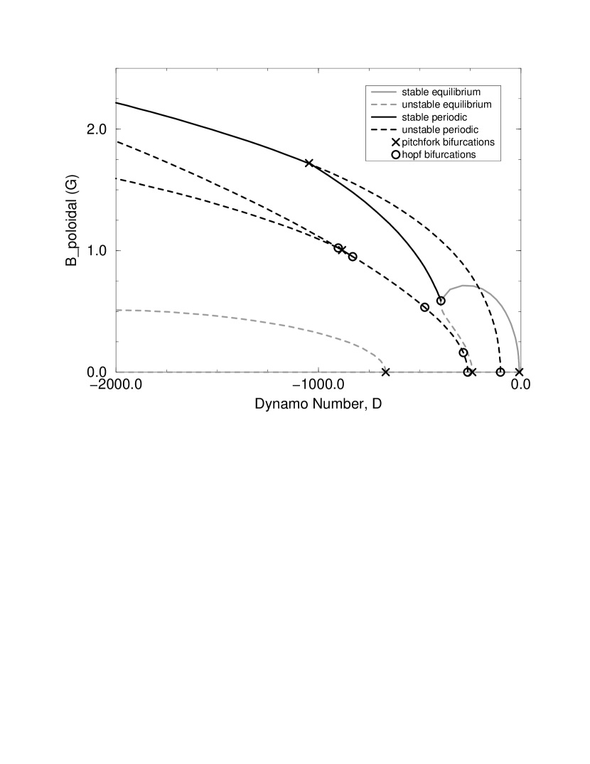
Figure 1: Bifurcation diagram for the one-layer system, $-2000<\mathcal{D}<0$, $\nu=0.5$, truncation level $N=24$. See further discussion in §3.

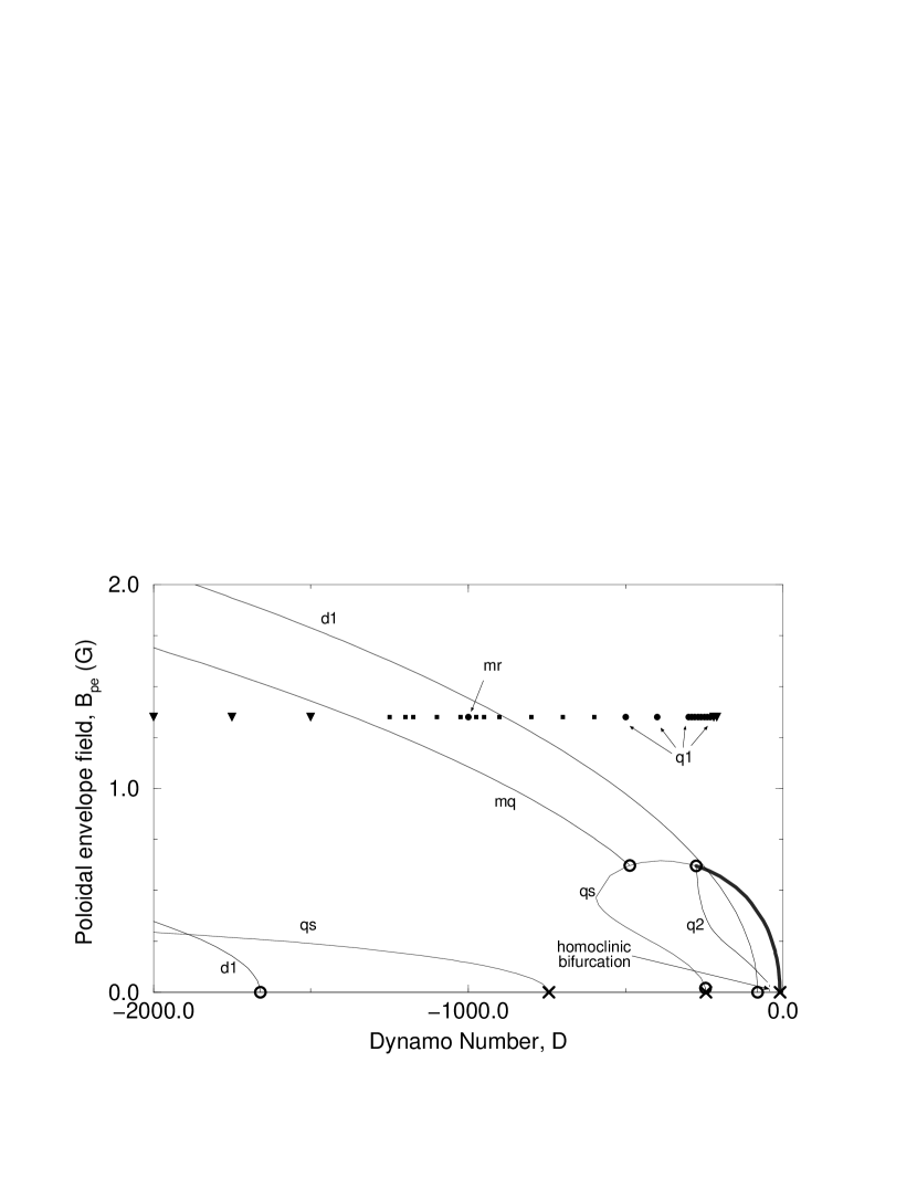
Figure 2: Bifurcation diagram for the two-layer system, $-2000<\mathcal{D}<0$, $\nu=0.5$, $\kappa=10^{-2}$, $\lambda=600$, truncation level $N=16$. See further discussion in §3.

Each curve in these diagrams represents a physically distinct solution of the equations; different solutions are characterised by the value of their poloidal magnetic field (in the $\alpha$ layer, in the case of the two-layer model), averaged over latitude and time. Each branch is labelled with its symmetry, as defined in Roald & Thomas (1997). Bifurcation points are marked.

The isolated points in the lower panels of Figure 2 (those plotted with filled circles, boxes, and triangles) show stable behaviour in parts of parameter space (specifically, for $\mathcal{D}\la-200$) where I was unable to get auto97 to lock onto a solution. These points were evaluated by time integration and at lower truncation ($N=8$), and so I have marked them with different symbols than the auto-computed branches. Furthermore, these solutions were classified qualitatively from the appearance of their Poincaré sections, and it should be understood that this technique is more art than algorithm, particularly for distinguishing between quasiperiodic and chaotic solutions. Because transients took a very long time to decay, I could only evaluate a few of these points for large negative $\mathcal{D}$. And lastly, note that their correct time average of their poloidal field strength is not determined, so they are all plotted at a single, arbitrary value.

4 Discussion

The graphs for the one-layer (Figure 1) and two-layer (Figure 2) models have many common features, as one would hope for related models.

• The first bifurcation from the trivial solution—the horizontal axis on the diagrams—is a quadrupole equilibrium, which loops back after a fold.

• There is another (unstable) quadrupole equilbrium, branching from the trivial solution near $\mathcal{D}=-700$.

• A periodic dipole solution branches from the trivial solution near $\mathcal{D}=-100$.

• A “mixed quadrupole” (mq) solution branches from the first equilibrium solution shortly before the fold.

Similar structure was also found by Jennings & Weiss (1991) in another 1D model with a different $\omega$-quenching prescription. The mixed quadrupole branch here produces a Sun-like dynamo mode (Figure 3).

Figure 3: Contour plots of the variation in time of the toroidal field, one-layer model, for the stable mq periodic branch at $\mathcal{D}=-1011$, $\nu=0.5$, truncation order $N=24$.

On the other hand, we must also note two important differences:

• the two-layer model (Figure 2) does not show an unstable periodic quadrupole solution bifurcating from the trivial solution anywhere in the range examined,

and critically,

• the stability of the steady quadrupole solution is destroyed in a subcritical Hopf bifurcation at $\mathcal{D}=-276$, before the supercritical bifurcation to the mq solution at $-486$.

The consequence of this last is that in the two-layer model, the solar-like mq mode is no longer stable, even though it exists in much the same form as in the one-layer version.

What do we have instead? The steady quadrupole mode loses stability after bifurcation with a quadrupole periodic mode. This mode tracks back toward smaller $\mathcal{D}$, and somewhere around $-60$ appears to be destroyed in a homoclinic connection with zero. At that point, a spray of stable unsteady solutions seems to be created, starting with a chaotic quadrupole. These do not appear to connect conventionally with any other solutions, and so I couldn’t get the continuation-method solver to lock on. Falling back to simple time-integration, we can determine the stable behaviour of the system from Poincaré sections. Figure 4

Figure 4: Poincaré sections for the two-layer system, $\nu=0.5$, $\kappa=10^{-2}$, $\lambda=600$, truncation $N=8$, taken on the section plane $B_{3}=0.005$. Each section is labelled with its dynamo number. Those for $\mathcal{D}=-300$ through $-250$ are single points, while $\mathcal{D}=-240$ and $-230$ are period-6 (with the six points of $-240$ too close together to be distinguishable at this scale). $\mathcal{D}=-220$ and $-210$ are apparently chaotic. All of these solutions have quadrupole symmetry.

shows solutions for ten different dynamo numbers at the lower end of the range that shows time-dependent behaviour. We start with two chaotic solutions at $\mathcal{D}=-220$ and $-210$, and progress through a series of periodic solutions. This is clearly the crudest first pass at a serious mathematical investigation of this system—for example, there are theorems that require some kind of very complicated dynamics to be going on between the period-6 orbit at $\mathcal{D}=-240$ and the period-1 orbit at $-250$—but pursuing it any farther seems unprofitable from a physical point of view.

These solutions have been marked on the bifurcation diagram, Figure 2. Figure 5 shows a typical simulated butterfly diagram from the quasiperiodic range.

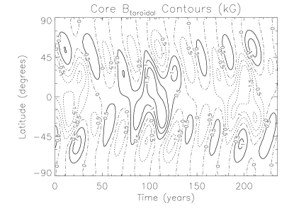
Figure 5: Contour plots of the variation in time of the shear-layer toroidal field, two-layer model, for the stable quadrupole quasiperiodic branch at $\mathcal{D}=-1200$, $\nu=0.5$, $\kappa=10^{-2}$, $\lambda=600$, truncation order $N=8$.

None of the computed modes of the two-layer model shows a Sun-like butterfly.

5 Conclusions

So, despite a recogniseably similar bifurcation structure, the stable behaviour of the two-layer model is entirely different from that of the one-layer version. This is not in itself a problem, because the two models do represent different physics. The concern, however, is that the only point to studying these simplified, or over-simplified, models is in the hope that something universal and robust can be identified from them and applied to our understanding of more sophisticated and computationally expensive models. Instead, however, we find almost frightening fragility.

Let me be careful in stating the conclusion here: I have shown here that one pair of admittedly unrealistic models are surprisingly sensitive to the addition of a simple bit of physics. This does not directly predict anything about the behaviour of more complex models. What it does force, however, is the indirect question: can we be confident that similar fragility does not occur in other models? Because if it does, the models are effectively useless. Having worked out quite a few bifurcation diagrams, my personal impression is we would be very lucky to find significant details in common between 1D models like these and more realistic dynamo models.

Jennings, R. L., & Weiss, N. O. 1991, , 252, 249 Moffatt, H. K. 1978, Magnetic Field Generation in Electrically Conducting Fluids, Cambridge: Cambridge Univ. Press Roald, C. B., & Thomas J. H. 1997, , 288, 551 Roald, C. B. 1998a, Ph.D. Thesis, University of Rochester, Rochester, NY, USA Roald, C. B. 1998b, , 300, 397