Generation of Magnetic Fields in the Relativistic Shock of Gamma-Ray-Burst Sources

Abstract

We show that the relativistic two-stream instability can naturally generate strong magnetic fields with $10^{-5}$–$10^{-1}$ of the equipartition energy density, in the collisionless shocks of Gamma-Ray-Burst (GRB) sources. The generated fields are parallel to the shock front and fluctuate on the very short scale of the plasma skin depth. The synchrotron radiation emitted from the limb-brightened source image is linearly polarized in the radial direction relative to the source center. Although the net polarization vanishes under circular symmetry, GRB sources should exhibit polarization scintillations as their radio afterglow radiation gets scattered by the Galactic interstellar medium. Detection of polarization scintillations could therefore test the above mechanism for magnetic field generation.

1. Introduction

Cosmological $\gamma$-ray bursts (GRB) are believed to be produced in the fireballs of very energetic explosions, when a large amount of energy, $E\sim 10^{51-54}\textrm{ erg}$, is released over a few seconds in a small volume in with a negligible baryonic load, $Mc^{2}\ll E$ (see Piran 1999 for a review). Most of the energy is eventually transferred to the baryons which are accelerated to ultra-relativistic velocities with a Lorentz factor $\gamma\simeq E/Mc^{2}\sim 10^{2}$–$10^{3}$ (e.g., Shemi & Piran (1990); Paczyński (1990)). A substantial fraction of the kinetic energy of the baryons is transferred to a non-thermal population of relativistic electrons through Fermi acceleration at the shock (Mészáros & Rees (1993)). The accelerated electrons cool via inverse Compton scattering and synchrotron emission in the post-shock magnetic fields and produce the radiation observed in GRBs and their afterglows (e.g., Katz (1994); Sari, Narayan, & Piran (1996); Vietri (1997); Waxman 1997a ; Wijers, Rees, & Mészáros (1997)). The shock could be either internal due to collisions between fireball shells caused by source variability (Paczyński & Xu 1994; Rees & Mészáros (1994)), or external due to the interaction of the fireball with the surrounding interstellar medium (ISM; Mészáros & Rees (1993)). The radiation from internal shocks can explain the spectra (Pilla & Loeb 1998) and the fast irregular variability of GRBs (Sari & Piran 1997a), while the synchrotron emission from the external shocks provides a successful model for the broken power-law spectra and smooth temporal behavior of afterglows (e.g., Waxman 1997a,b). In both cases, strong magnetic fields are required behind the shocks at all times in order to fit the observational data.

The properties of the synchrotron emission from GRB shocks are determined by the magnetic field strength, $B$, and the electron energy distribution behind the shock. Both of these quantities are difficult to estimate from first principles, and so the following dimensionless parameters are often used to incorporate modeling uncertainties (Sari, Narayan, & Piran (1996)),

$$\epsilon_{B}\equiv\frac{U_{B}}{e_{\rm th}},\qquad\epsilon_{e}\equiv\frac{U_{e}}{e_{\rm th}}.$$ (1)

Here $U_{B}={B^{2}}/{8\pi}$ and $U_{e}$ are the magnetic and electron energy densities and $e_{\rm th}=nm_{p}c^{2}(\bar{\gamma}_{p}-1)$ is the total thermal energy density behind the shock; where $m_{p}$ is the proton mass, $n$ is the proton number density, and $\bar{\gamma}_{p}$ is the mean thermal Lorentz factor of the protons. The observed afterglow spectra and lightcurves typically yield values of the magnetic energy parameter ranging from $\epsilon_{B}\sim 0.1$ (Waxman 1997; Wijers & Galama 1998), down to $10^{-2}$ (Granot et al. 1998) or even $\epsilon_{B}\sim 10^{-5}$ (Galama et al. 1999; Vreeswijk et al. (1999)) — all below the equipartition limit $\epsilon_{B}\sim 1$.

The existence of strong magnetic fields is naturally expected in the compact environments of potential GRB progenitors. First, the field might originate from a highly magnetized stellar remnant, such as a neutron star, with $B\lesssim 10^{16}\textrm{ gauss}$. Second, a turbulent magnetic dynamo could amplify a relatively weak seed magnetic field in the vicinity of the progenitor. This process, however, requires the turbulence to be anisotropic and have a nonzero total helicity, ${\bf v\cdot(\nabla\times v)}\not=0$. A similar mechanism, called the $\alpha$-$\Omega$-dynamo, might operate in rapidly rotating objects (Thompson (1994), see also Mészáros, Laguna, & Rees (1993)). Finally, the magnetic shearing instability (Balbus & Hawley (1991)) could amplify the magnetic field (but not the flux) in strongly sheared flows. The $e$-folding time for this instability is approximately the rotation period, which decreases with radius as $R^{-2}$ due to angular momentum conservation in the outflowing wind. Thus, being possibly important in the early stages of the fireball expansion (Narayan, Paczyński, & Piran (1992)), this instability is inefficient at large radii, where its $e$-folding time greatly exceeds the dynamical time of the fireball.

In contrast to such progenitor environments where large magnetic fields are natural, there is currently no satisfactory explanation for the origin of the strong magnetic fields required in GRB shocks (see discussions in Thompson (1994); Mészáros, Laguna, & Rees (1993); Sari, Narayan, & Piran (1996)). Compression of the ISM magnetic field in external shocks yields a field amplitude $B\sim\gamma B_{\rm ISM}\sim 10^{-4}(\gamma/10^{2})\textrm{ gauss}$, which is too weak (Sari, Narayan, & Piran (1996)) compared to the required equipartition value $B_{eq}\sim 50(\gamma/10^{2})(n_{\rm ISM}/1~{}{\rm cm^{-3}})^{1/2}\textrm{ gauss}$, and can account only for $\epsilon_{B}=(B/B_{eq})^{2}\lesssim 10^{-11}$. Alternatively, some magnetic flux might originate at the GRB progenitor and be carried by the outflowing fireball plasma (or by a precursor wind). Because of flux freezing, the field amplitude would decrease as the wind expands. In this case, only a progenitor with a rather strong magnetic field $\sim 10^{16}\textrm{ gauss}$ might produce sufficiently strong fields during the GRB emission. However, since the field amplitude scales as $B\propto V^{-2/3}$ for an expanding shell of volume $V$, even a highly magnetized plasma at $R\sim 10^{7}\textrm{ cm}$ would possess only a negligible field amplitude of $\sim 10^{-2}\textrm{ gauss}$, or $\epsilon_{B}\lesssim 10^{-7}$, at a radius of $R\gtrsim 10^{16}\textrm{ cm}$, where the afterglow radiation is emitted (see also Mészáros, Laguna, & Rees (1993)). Moreover, the emitting material behind the external shock is continuously replenished by the ISM, and so the field originally carried by the fireball ejecta cannot account for the afterglow radiation.

None of the above mechanisms is capable of generating near equipartition magnetic fields in the external shocks which produce the delayed afterglow emission. In this paper, we propose a different, universal mechanism of magnetic field generation in GRB shocks. It involves the relativistic generalization of the two-stream (Weibel) instability in a plasma. This instability is driven by the anisotropy of the Particle Distribution Function (PDF) and, hence, could operate in both internal and external shocks. Our main results are as follows:

1. The characteristic $e$-folding time in the shock frame for the instability is $\sim 10^{-7}\textrm{ s}$ for internal shocks and $10^{-4}\textrm{ s}$ for external shocks. This time is much shorter than the dynamical time of GRB fireballs.

2. The generated magnetic field is randomly oriented in space, but always lies in the plane of the shock front.

3. The instability is powerful. It saturates only by nonlinear effects when the magnetic field amplitude approaches equipartition with the electrons (and possibly with the ions).

4. The instability isotropizes the PDF and, thus, effectively heats the electrons and protons.

5. The characteristic coherence scale of the generated magnetic field is of the order of the relativistic skin depth, i.e. $\sim 10^{3}\textrm{ cm}$ for internal shocks and $\sim 10^{5}\textrm{ cm}$ for external shocks. This scale is much smaller than the spatial scale of the source.

6. The mean free path for Coulomb collisions is larger than the fireball size. However, the randomness of the generated magnetic field provides effective collisions due to pitch angle scattering of the particles in an otherwise collisionless plasma and, thus, justifies the use of the magneto-hydrodynamic (MHD) approximation for GRB shocks. The magnetic fields communicate the momentum and pressure of the outflowing fireball plasma to the ambient medium and define the shock boundary.

The above mechanism results in tangential magnetic fields near the apparent limb of the source. Hence, the long-term synchrotron emission from the limb would be linearly polarized along the radial direction relative to the source center. Although the net polarization of a circularly symmetric source is zero, scattering of the radio afterglow emission of GRBs by the intervening Galactic interstellar medium would break the symmetry in the source image and result in polarization scintillations. This effect can be used to test the reality of our proposed mechanism for the generation of magnetic fields in GRB blast waves.

The outline of the paper is as follows. The physical mechanism of the instability is discussed in §2. The generation of magnetic fields in internal and external shocks is discussed in §3. In §4 we predict the polarization scintillation signal in our model. Finally, §5 summarizes our main conclusions.

2. The Two-Stream Instability

The instability under consideration was first predicted by Weibel (1959) for a non-relativistic plasma with an anisotropic distribution function. The simple physical interpretation provided later by Fried (1959) treated the PDF anisotropy more generally as a two-stream configuration of a cold plasma. Below we give a brief, qualitative description of this two-stream magnetic instability.

Let us consider, for simplicity, the dynamics of the electrons only, and assume that the protons are at rest and provide global charge neutrality. The electrons are assumed to move along the $x$-axis (as illustrated in Figure 1) with a velocity ${\bf v}=\pm{\bf\hat{x}}v_{x}$ and equal particle fluxes in opposite directions along the $x$-axis (so that the net current is zero). Next, we add an infinitesimal magnetic field fluctuation, ${\bf B}={\bf\hat{z}}B_{z}\cos(ky)$. The Lorentz force, $-e{{{\bf v}\over c}\times{\bf B}}$, deflects the electron trajectories as shown by the dashed lines in Figure 1. As a result, the electrons moving to the right will concentrate in layer I, and those moving to the left – in layer II. Thus, current sheaths form which appear to increase the initial magnetic field fluctuation. The growth rate is $\Gamma=\omega_{\rm p}v_{y}/c$, where $\omega_{\rm p}^{2}=(4\pi e^{2}n/m)$ is the non-relativistic plasma frequency (Fried (1959)). Similar considerations imply that perpendicular electron motions along $y$-axis, result in oppositely directed currents which suppress the instability. The particle motions along ${\bf\hat{z}}$ are insignificant as they are unaffected by the magnetic field. Thus, the instability is indeed driven by the PDF anisotropy and should quench for the isotropic case.

The Lorentz force deflection of particle orbits increases as the magnetic field perturbation grows in amplitude. The amplified magnetic field is random in the plane perpendicular to the particle motion, since it is generated from a random seed field. Thus, the Lorentz deflections result in a pitch angle scattering which makes the PDF isotropic. If one starts from a strong anisotropy, so that the thermal spread is much smaller than the particle bulk velocity, the particles will eventually isotropize and the thermal energy associated with their random motions will be equal to their initial directed kinetic energy. This final state will bring the instability to saturation.

We note the following points about the nature of the instability:

1. The instability is aperiodic, i.e., ${\rm Re}\,\omega=0$. Thus, it can be saturated by nonlinear effects only, and not by kinetic effects such as collisionless damping or resonance broadening. Hence, the magnetic field can be amplified up to high values.

2. Despite its intrinsically kinetic nature, the instability is non-resonant, i.e., it is impossible to single out a group of particles that is responsible for the instability. Since the bulk of the plasma participates in the process, the energy transferred to the magnetic field could be comparable to the total kinetic energy of the plasma. Hence, the instability is powerful.

3. The instability is self-saturating. It continues until all the free energy due to the PDF anisotropy is transferred to the magnetic field energy.

4. The generated magnetic field always lies in the plane perpendicular to the initial anisotropy axis of the PDF, i.e., to the shock propagation direction.

5. The produced magnetic field is randomly oriented in the shock plane. The Lorentz forces randomizes particle motion over the pitch angle and, hence, introduces an effective scattering process into the otherwise collisionless system. This validates the use of the MHD approximation in the study of collisionless GRB shocks.

Sagdeev & Galeev (1969) and Moiseev & Sagdeev (1963) provide a kinetic, non-relativistic treatment of the instability in both the linear and the quasi-linear regimes, and apply the theory of collisionless shocks to space plasmas. In the next section we will extend their analysis to the case of ultra-relativistic GRB shocks.

3. Magnetic Field Generation in GRB Shocks

We consider a GRB shock front expanding at a Lorentz factor, $\gamma_{\rm sh}$, behind which the particles have a thermal Lorentz factor, $\bar{\gamma}$. In this section, we will derive equations which are equally applicable to electrons and protons, whichever species dominates the growth of the instability. Later, we shall use the subscripts “$e$” and “$p$” to denote electrons and protons, respectively. We calculate all quantities in the comoving frame of the shock.

A fully kinetic, relativistic treatment of the magnetic two-stream (Weibel) instability is a complicated task. The dispersion relation for a simplified “water-bag” PDF was derived by Yoon & Davidson (1987) and is given by equation (A2) in Appendix A. This dispersion relation implies that only a range of modes above a critical wavelength will grow [cf. Eq. (A3)]. Naturally, the mode with the largest growth rate, $\Gamma_{\rm max}$, dominates and sets the characteristic length-scale of the magnetic field fluctuations, $\lambda\sim k_{\rm max}^{-1}$. The ultra-relativistic expressions for $\Gamma_{\rm max}$ and $k_{\rm max}$ are given by equation (A5) for a strong initial anisotropy. We write the corresponding $e$-folding time and correlation length of the field as

$$\tau\simeq\frac{\gamma_{\rm sh}^{1/2}}{\omega_{\rm p}},\quad\lambda\simeq 2^{1/4}\frac{c\bar{\gamma}^{1/2}}{\omega_{\rm p}}.$$ (2)

We can now estimate the nonlinear saturation amplitude of the magnetic field. The instability is due to the free streaming of particles. As the field amplitude grows, the transverse deflection of particles gets stronger, and their free streaming across the field lines is suppressed. The typical curvature scale for the deflections is the Larmor radius, $\rho=v_{\bot B}/\Omega_{\rm c}\simeq(\gamma_{\bot B}^{2}-1)^{1/2}mc^{2}/eB$, where $v_{\bot B}$ and $\gamma_{\bot B}$ are the transverse velocity and Lorentz factor of a particle relative to the local magnetic field. On scales larger than $\rho$, particles can only move along field lines. Hence, when the growing magnetic fields become such that $k_{\rm max}\rho\sim 1$, the particles are magnetically trapped and can no longer amplify the field. Assuming an isotropic particle distribution at saturation ($\gamma_{\bot B}\sim\bar{\gamma}$), this condition can be re-written as

$$\frac{B^{2}/8\pi}{mc^{2}n(\bar{\gamma}-1)}\sim\frac{(\bar{\gamma}+1)}{2\sqrt{2}\,\bar{\gamma}}.$$ (3)

For ${\bar{\gamma}}\gg 1$, this corresponds to a magnetic energy density close to equipartion with the amplifying particles. Interestingly, one may obtain the same result following a different analysis. First, the instability leads to a growth of the field amplitude [as given by the last term in Eq. (A1), $\sim{\bf v\cdot}\partial_{\bf x}f$]. Second, nonlinearity leads to the transfer of energy to shorter wave lengths, $k>k_{\rm crit}$, where the fluctuations are damped [as described by the second term in Eq. (A1), $\sim(e/c){\bf v\times B\cdot}\partial_{\bf p}f$]. Thus, the steady value of $B$ is determined by balancing these two processes. Equating these two terms and replacing $\partial_{x}$ by $k_{\rm crit}\simeq k_{\rm max}/\sqrt{2}\sim\rho_{p}/\sqrt{2}$, yields

$$v_{\bot B}k_{\rm crit}f\sim v_{\bot B}eBf/mc^{2}\gamma_{\bot B}.$$ (4)

The field strength estimated here is equivalent to that given in equation (3) to within a factor of order unity.

Direct computer simulations of the instability in both non-relativistic and relativistic electron plasmas confirm that the saturation occurs at slightly sub-equipartition values of $B$ (see, e.g., Califano et al. (1998); Kazimura et al. 1998; Yang et al. (1994); Wallace & Epperlein (1991)),

$$\frac{B^{2}/8\pi}{mc^{2}n(\bar{\gamma}-1)}\equiv\eta\sim 0.01-0.1\,.$$ (5)

where we introduced the efficiency factor $\eta\lesssim 0.1$. The precise saturation level depends on the nonlinear modification of the PDF during the instability which is not accounted for by our linear analysis. We shall retain the efficiency factor, $\eta$, in our estimates.

Note that the thermal Lorentz factor of particles, $\bar{\gamma}$, varies in time as the instability develops. Due to particle scattering by the generated magnetic fields, an initially highly anisotropic PDF with $\bar{\gamma}\ll\gamma_{\rm sh}$ will eventually evolve to an isotropic, ring-like distribution, for which $\bar{\gamma}\simeq\gamma_{\rm sh}$. Thus, the spatial scale and amplitude of the resultant magnetic field, given by equations (2) and (5), will evolve during the lifetime of the instability because they are functions of $\bar{\gamma}$. In estimating these values at a GRB shock when the instability saturates, we take $\bar{\gamma}\simeq\gamma_{\rm sh}$. The $e$-folding time for the instability is independent of $\bar{\gamma}$ in the case of strong anisotropy. In the case of weak anisotropy, $\bar{\gamma}\approx\gamma_{\rm sh}$, the “water-bag” model used here is formally invalid, but the comparison of the ultra-relativistic results with non-relativistic results (e.g., Moiseev & Sagdeev 1963) suggests that the instability quenches and the $e$-folding time scales as

$$\tau\simeq\lambda/c\propto\left[(\epsilon_{\|}-\epsilon_{\perp})/\epsilon_{\|}\right]^{-3/2},$$ (6)

where $\epsilon_{\|}$ and $\epsilon_{\perp}$ are the average energies of particle motions along the direction of shock propagation and transverse to it. The field correlation length follows a similar scaling.

The diffusive decay time of the generated magnetic field is $\tau_{\rm diff}\simeq 1/\eta_{B}k_{\rm max}^{2}$, where $\eta_{B}=mc^{2}\nu_{\rm coll}/4\pi ne^{2}$ is the magnetic diffusivity and $\nu_{\rm coll}$ is the particle collision frequency. Hence, the diffusion time

$$\tau_{\rm diff}\simeq\bar{\gamma}/\nu_{\rm coll},$$ (7)

is much longer than the fireball expansion time since the particle collision frequency in the fireball plasma is negligible. Thus, the magnetic field is not expected to dissipate its energy Ohmically over the fireball lifetime. Note that magnetic fields cannot be produced during the optically-thick phase of the fireball, because Compton scattering on the photons rapidly removes any anisotropy of the PDF. Next, we consider two types of GRB shocks in which magnetic fields might be generated.

3.1. Internal Shocks due to Shell Collisions Inside the Fireball

Rapid variability of a GRB source results in a fireball which is composed of thin layers (shells) moving with different Lorentz factors. To produce the observed non-thermal $\gamma$-ray spectrum, the shells must collide at sufficiently large radii where the internal shock region is optically-thin to both Compton scattering and $e^{+}e^{-}$-pair production. The collision should also occur before the fireball slows-down on the ambient medium. These conditions imply that the internal shock be mildly relativistic, with a Lorentz factor $\gamma_{\rm int}$ of order a few in the center of mass frame of the colliding shells (see Piran 1999 for more details). Prior to a collision, the electrons and protons in the colliding shells are cold relative to their bulk Lorentz factor, $\bar{\gamma}_{e,p}\lesssim\gamma_{\rm int}$. As typical parameters for the shells we assume a plasma density of $n\approx 3\times 10^{10}\textrm{ cm}^{-3}$, $\gamma_{\rm int}=4$, and initial thermal Lorentz factors $\bar{\gamma}_{p,e}\approx 2$ (see e.g., Piran 1999; Pilla & Loeb (1998)). The plasma frequencies for the electrons and protons are given by the relations, ${\omega_{\rm p}}_{e}=9.0\times 10^{3}n^{1/2}\textrm{ s}^{-1}$ and ${\omega_{\rm p}}_{p}=2.1\times 10^{2}n^{1/2}\textrm{ s}^{-1}$, where $n$ is in $\textrm{ cm}^{-3}$.

For simplicity, we consider the collision of two identical shells. In the center of mass frame, the interaction of these collisionless shells yields a state of two inter-penetrating plasma streams, which is readily unstable to the generation of magnetic fields. Since ${\omega_{\rm p}}_{e}\gg{\omega_{\rm p}}_{p}$, the instability grows faster for the electrons than for the protons and so the electrons dominate the magnetic field generation process at early times. The electron instability saturates when the magnetic energy density becomes comparable to the electron energy density, $\gamma_{\rm int}nm_{e}c^{2}$. This energy is still much smaller than that associated with the protons. Thus, when the instability saturates for the electrons, it could still continue on a longer time-scale for the protons. The protons dominate energetically and could lead to near equipartition magnetic energy with

$$\epsilon_{B}\lesssim\eta\sim 0.1.$$ (8)

From equation (2) we get the characteristic scale length and growth time of the instability for the protons,

$$\lambda \simeq 2\times 10^{3}\left(\frac{n}{3\times 10^{10}\textrm{ cm}^{-3}}\right)^{-1/2}\left(\frac{\gamma_{\rm int}}{4}\right)^{1/2}\textrm{ cm},~{}~{}~{}~{}~{}~{}~{}$$ (9a)

$$\tau \simeq 6\times 10^{-8}\left(\frac{n}{3\times 10^{10}\textrm{ cm}^{-3}}\right)^{-1/2}\left(\frac{\gamma_{\rm int}}{4}\right)^{1/2}\textrm{ s}.$$ (9b)

These quantities are decreased by a factor of $(m_{p}/m_{e})^{1/2}=43$ for the electrons.

The generation of magnetic fields in counter-streaming, electron-positron plasmas has been extensively studied numerically using particle-in-cell codes (e.g., Kazimura et al. (1998); Califano et al. (1998); Yang et al. (1994)). A clear visual demonstration of the magnetic field amplification process is provided by Figure 2 of Kazimura et al. (1998). The rapid generation of a strong, small-scale magnetic field occurs at the interface of the colliding streams, and is followed by the gradual modification of the field structure around the interface, due to the nonlinear saturation and relaxation of the particle velocity anisotropy. The inferred value of $\eta\sim 0.01-0.1$ is generic (Kazimura et al. (1998); Yang et al. (1994)). The amplication process produces also random electric fields with an energy density that is at most comparable to that of the magnetic component, $\langle E^{2}\rangle\sim(v/c)\langle B^{2}\rangle$ (Kazimura et al. (1998)).

Unfortunately, no simulations were performed so far for colliding electron-proton plasmas. Numerical simulations of a plasma with species of somewhat different masses suggests that the energetics of the process is indeed dominated by the heavier species (Arons (1996)). Nevertheless, direct relativistic simulations with dynamical protons and electrons are required in order to assess the saturation amplitude of the magnetic field in GRB shocks of different properties.

If the colliding shells do not possess similar densities, then the growth rate of the instability decreases or even shuts off beyond a particular density contrast, as discussed in Appendix B. In this regime, the shock may be dominated by electrostatic (Langmuir) turbulence. Unless the outflowing plasma is already contaminated by strong magnetic fields, the synchrotron emission from the collision of shells with very different densities would therefore be weak.

3.2. External Shock due to the Interaction of the Fireball with the ISM

Eventually, the fireball slows down due to its interaction with the surrounding ISM. The external shock produced by this interaction yields the delayed afterglow emission and is assumed to carry a strong magnetic field. As the shock propagates into the ISM, the fresh electrons and protons are reflected from the magnetized shock front back into the ISM. Thus, a two-stream state forms in the comoving frame of the shock and a magnetic field is amplified in the ISM, just in front of the shock.

We assume that the fraction of reflected particles is of order unity, and so the above two-stream state is analogous to that produced in internal shocks. The instability first acts on the electrons. The correlation scale and saturation amplitude of the field are given by equations (2) and (5). Since the magnetic field is generated upstream and then transported downstream, we need to take account of the compression factor at the shock. Given the jump conditions for a relativistic shock, we have $\lambda=\lambda^{\prime}/4\gamma_{\rm sh}$ (where “prime” denotes the parameter in front of the shock), while the ratio of the magnetic to thermal energy remains constant. For an ISM density $n_{\rm ISM}\approx 1\textrm{ cm}^{-3}$, we therefore get the following parameters behind the shock,

$${\epsilon_{B}}_{e} = \eta\,\left(\frac{m_{e}}{m_{p}}\right)\simeq 5.5\times 10^{-5}\eta_{.1},$$ (10a)

$$\lambda_{e} = 3\times 10^{5}\left(\frac{\gamma_{\rm sh}}{10}\right)^{-1/2}\left(\frac{n_{\rm ISM}}{1\textrm{ cm}^{-3}}\right)^{-1/2}\textrm{ cm},~{}~{}~{}~{}~{}~{}~{}$$ (10b)

$$\tau_{e} = 4\times 10^{-4}\left(\frac{\gamma_{\rm sh}}{10}\right)^{1/2}\left(\frac{n_{\rm ISM}}{1\textrm{ cm}^{-3}}\right)^{-1/2}\textrm{ s}.$$ (10c)

where $\eta_{.1}\equiv(\eta/0.1)$ and the subscript “$e$” denotes amplification of the magnetic field by the electrons only. The magnetic energy parameter is still normalized relative to the proton thermal energy.

When the instability of the electrons saturates, further amplification by the protons may become important. The magnetic field is amplified in a thin layer in front of the shock, the width of which is of order the Larmor radius of the protons at the shock. The time available for field amplification is, thus, roughly the crossing time, $t_{\rm amp}\sim\rho_{p}/c\sim\bar{\gamma}_{p}(\bar{\gamma}_{e}\gamma_{\rm sh}\eta)^{-1/2}(m_{p}/m_{e})^{1/2}(B_{{\rm sat,}e}/B)\tau_{p}\sim 3(m_{p}/m_{e})^{1/2}(B_{{\rm sat,}e}/B)\tau_{p}$, where $B_{{\rm sat,}e}$ denotes the field strength after saturation on the electrons [as given by Eq. (10a)]. On the other hand, the growth of the field to a sub-equipartition amplitude with the protons would take at least $t_{\rm growth}=\tau_{p}\ln(B_{{\rm sat,}p}/B_{{\rm sat,}e})\sim\tau_{p}\ln(m_{p}/m_{e})^{1/2}\sim 3.8\tau_{p}$, i.e. comparable to the time available for the amplification of $B_{{\rm sat,}e}$ up to $B_{{\rm sat,}p}=(m_{p}/m_{e})^{1/2}B_{{\rm sat,}e}$. However, since the growth of the field near saturation is slower than that during the linear stage of the process, the Weibel instability may not be able to build the field up to equipartition with the protons and yield $\epsilon_{B}\sim\eta$. Whether maximal amplification of the magnetic field can occur in this environment is uncertain and can be found only through detailed numerical simulations. We thus conclude that the most robust prediction for the value of the magnetic field energy is $\epsilon_{B}\sim\eta(m_{e}/m_{p})$, but somewhat higher values are also possible, so that

$$5\times 10^{-5}\eta_{.1}\lesssim\epsilon_{B}\lesssim 0.1\eta_{.1}.$$ (11)

The predicted range of $\epsilon_{B}\sim 10^{-1}$–$10^{-5}$ matches the results from modeling of recent afterglow data. Wijers & Galama (1998) show that X-ray to radio spectrum of GRB970508 afterglow is consistent with the values of $\epsilon_{B}\sim 0.07$, indicating the proton dominated regime of field generation. The field energy density for GRB990123 and GRB971214 is estimated to be $\epsilon_{B}\sim 10^{-5}$ (Galama et al. (1999)), and for GRP980703 $\epsilon_{B}\sim 6\times 10^{-5}$ (Vreeswijk et al. (1999)), consistently with the electron dominated regime.

4. Polarization Scintillations

In the previous section, we have found that the characteristic time it takes the magnetic field to grow up to equipartition values is orders of magnitude shorter than the dynamical time-scale of GRB shocks. Hence, the growth of the field does not have observational consequences. Similarly, the typical correlation length of the magnetic field is much smaller than the source size and cannot be resolved. Thus, conventional light-curve observations are unable to test the magnetic instability mechanism. However, polarization measurements might be more promising, as we show next.

4.1. General Considerations

Synchrotron radiation produced by relativistic electrons is known to be highly polarized, predominantly in the direction perpendicular to the local magnetic field (Ginzburg (1989); Rybicki & Lightman (1979)). It was shown in §2 that the generated magnetic field is randomly oriented in the plane of the shock front.

The afterglow radiation emitted by any infinitesimal section of the GRB blast wave is relativistically beamed to within an opening angle $\theta_{\rm b}\sim\gamma_{\rm sh}^{-1}\ll 1$. Hence, an external observer sees a conical section of the fireball, as defined by this opening angle. In addition, the rapid deceleration of the fireball reduces its surface brightness as it expands. For a particular observed time, emission along the line-of-sight axis to the source center suffers from the shortest geometric time-delay, and hence originates at a larger radius and is dimmer than slightly off-axis emission. The source therefore appears as a narrow limb-brightened ring (Waxman 1997c; Sari 1998; Panaitescu & Meszaros 1998; Granot et al. 1998a). The outer cut-off of the ring is set by the sharp decline in the relativistic beaming at angles greater than $\gamma_{\rm sh}^{-1}$. Interestingly, the shock surface appears to a distant observer as almost perfectly aligned along the line-of-sight at the edge of the ring. This effect results from relativistic aberration (Rybicky & Lightman 1979, p. 110), i.e. the Lorentz transformation of angles from the shock frame (in which the normal to the shock surface is inclined at an angle $\gamma_{\rm sh}^{-1}$ relative to the line-of-sight) to the observer frame. Therefore, at the limb-brightened edge of the ring, the small-scale magnetic field is oriented tangentially on the sky. Consequently, the random magnetic field does not average-out but rather produces linear polarization which is oriented radially from the center at any point on the ring. The resulting synchrotron radiation obtains a degree of polarization of

$$\pi_{\rm syn}=\frac{p_{e}+1}{p_{e}+7/3}\simeq 72\%$$ (12)

for the typical value of the power-law index, $p_{e}=2.5$, of the electron energy distribution, $dN_{e}/d\gamma_{e}\propto\gamma_{e}^{-p_{e}}$, in GRB sources.

The two-stream mechanism for the amplification of the magnetic field can be tested only if the source is resolved, since the net polarization of a circularly-symmetric image is zero. There are two ways for resolving a compact GRB source: (i) scintillations of radio afterglows due to electron density irregularities in the ISM of the Milky Way galaxy (Goodman 1997); and (ii) gravitational microlensing due to an intervening star along the line-of-sight (Loeb & Perna 1998). Since lensing occurs only rarely, we focus our discussion on the first method. Observations of interstellar scintillations probe angular scales of order a few micro-arcseconds ($\ \mu{\rm as}$), far below the VLBI resolution ($\sim 300\ \mu{\rm as}$).

The interstellar scintillations arise when fluctuations in the electron density randomly modulate the refractive index of the turbulent ISM. As a result of random focusing and diffraction of the electromagnetic wave, a point source produces a spatial pattern of random bright and dim spots — the speckle pattern. The source brightness fluctuates as the observer moves across the pattern. The characteristic angular correlation length of the pattern, $\theta_{0}$, is set by the statistical properties of the ISM turbulence. If, however, the source is extended, then the overall pattern is obtained from the superposition of the incoherent patterns of its individual parts. Thus, if the angular size of the source, $\theta_{\rm s}$, is larger than the characteristic scale of the speckles, namely $\theta_{\rm s}>\theta_{0}$, then the intensity fluctuations wash-out and the scintillation amplitude diminishes. The observations of a late-time decline in the amplitude of intensity scintillations for the radio afterglows GRB970508 (Frail et al. (1997); Waxman, et al. (1998)) and GRB980329 (Taylor et al. (1998)) provide an estimate for the shock radius, $R_{\rm s}\sim 10^{17}\textrm{ cm}$ at times of $\sim 1$ month and $\sim 2$ weeks after these bursts, respectively. These estimates are consistent with the simplest fireball model predictions.

The Weibel instability mechanism predicts that different segments of the ring-like source emit synchrotron radiation which is linearly polarized along the radial axis, so that the net polarization vanishes when averaged over the source. If $\theta_{\rm s}\ll\theta_{0}$, the source is effectively point-like and hence symmetric. This regime is characterized by strong intensity scintillations and weak polarization fluctuations. In contrast, when $\theta_{\rm s}>\theta_{0}$, different parts of the source are mapped differently, and the source is resolved. As the earth moves through the scintillation pattern, an observer will measure fluctuations in the direction and amplitude of the polarization, while the intensity would vary only weakly due to the overlap of the separate speckle patterns. The polarization scintillations should therefore be strong when the flux fluctuations are weak.

We consider two types of scintillations, diffractive and refractive (Goodman & Narayan (1985); Blandford & Narayan (1985)). Diffractive scintillations occur when the source is nearly point-like, $\theta_{\rm s}\ll\theta_{\rm d}$, relative to

$$\theta_{\rm d}\simeq 3\left(\frac{\nu}{10\textrm{ GHz}}\right)^{-11/5}\ \mu{\rm as},$$ (13)

which is the diffraction angle for a typical scattering measure of $10^{-3.5}{\rm m}^{-20/3}~{}{\rm kpc}$ (Goodman (1997)). The flux modulation amplitude in the strong scattering regime is close to $100\%$. For a Kolmogorov spectrum of ISM turbulence, the characteristic speckle length is

$$\theta_{0}\simeq 2.3\left(\frac{\nu}{10\textrm{GHz}}\right)^{6/5}\ \ \mu{\rm as},$$ (14)

assuming a scattering screen distance of $\sim 1~{}{\rm kpc}$ and a typical scattering measure of $10^{-3.5}{\rm m}^{-20/3}~{}{\rm kpc}$ (Goodman 1997). The time-scale for diffractive scintillations is

$$t_{\rm diff}\simeq 3\left(\frac{\nu}{10\textrm{ GHz}}\right)^{6/5}\textrm{ hr}$$ (15)

if the transverse velocity of the line of sight is dominated by the earth with $v_{\bot}\simeq 30\textrm{ km s}^{-1}$. As long as $\theta_{\rm s}\ll\theta_{0}$, the polarization is close to zero, but when the source approaches the speckle correlation length, $\theta_{\rm s}\sim\theta_{0}$, the polarization scintillations could grow up to a large amplitude, of order a few tens of percents [cf. Eq. (12)]. For these scintillations to be detected, the source must be observed at relatively low frequencies (Goodman (1997)), namely $\nu\lesssim 10\textrm{GHz}$ for typical ISM conditions. Unfortunately, the synchrotron self-absorption often occurs at frequencies below 5 GHz, and so the afterglow might be fainter at these low frequencies, making the detection of polarization scintillations more difficult. In addition, the source image resembles more a filled disk rather than a hollow ring at low frequencies (Granot et al. 1998a). The unpolarized radiation emitted near the center of the disk will thus lower the overall degree of polarization.

As the source gets larger, $\theta_{\rm s}\gg\theta_{\rm d}$, the diffractive effect weakens, and the scintillations are dominated by the refractive effect, which yields only modest intensity fluctuations with an amplitude $\sim 10\%$. The polarization fluctuations in this regime have a corresponding amplitude of only a few percents. The characteristic time-scale for the refractive modulation is

$$t_{\rm ref}\simeq 14\left(\frac{\theta_{\rm eff}}{10\ \mu{\rm as}}\right)\textrm{ hr},$$ (16)

where $\theta_{\rm eff}$ is the effective size of the source (see Goodman (1997) for details).

4.2. Polarization Scintillations: Formalism

The properties of the radiation field are fully described by four scalar parameters — the Stokes parameters (Ginzburg (1989)), which are additive for incoherent sources. For synchrotron radiation produced by relativistic electrons, these parameters include the intensity $I$ and

$$Q = I\,\cos 2\psi\,\cos 2\chi,$$ (17a)

$$U = I\,\cos 2\psi\,\sin 2\chi,$$ (17b)

$$V = 0.$$ (17c)

The last parameter, $V$, describes circular polarization while $Q$ and $U$ describe linear polarization. $\chi$ is the angle between the polarization axis and an arbitrary fixed direction in the sky and $\cos 2\psi=(I_{\|}-I_{\perp})/(I_{\|}+I_{\perp})$ is the difference between the radiation intensity along the two orthogonal axes of polarization divided by the sum (see Ginzburg (1989); and Rybicki & Lightman (1979), p. 180). Both $\chi({\bf r})$ and $\psi({\bf r})$ are determined by the source, but are not affected by the scintillations. The degree of polarization is defined as

$$\pi=\left(Q^{2}+U^{2}+V^{2}\right)^{1/2}/I.$$ (18)

Given a power spectrum of electron density fluctuations in the ISM, the statistics of speckles in a scintillation pattern is usually characterized by the second moment correlation of the complex electric field of the electromagnetic radiation,

$${\sf W}(\Delta{\bf x}) = {\overline{E({\bf x})E^{*}({\bf x}+\Delta{\bf x})}}$$ (19)

$$\propto \exp\left[-D_{\varphi}(\Delta{\bf x})/2\right]$$

$$\propto \exp\left[-const\times(|\Delta{\bf x}|)^{\beta-2}\right],$$

where ${\bf x}$ and $\Delta{\bf x}$ are two-dimensional vectors on the plane normal to the line of sight, the “bar” denotes an ensemble average, and $\beta$ is the power-law index of the power spectrum of electron density fluctuations, $|\delta n_{e}(q)|^{2}\propto q^{\beta}$ with $q$ being the spatial wave-number. The quantity $D_{\varphi}$ is the phase structure function which yields the phase shift along different paths and is determined by the ISM turbulence. The inferred value of $\beta$ for the Galactic ISM is somewhat uncertain but close to the Kolmogorov theory prediction $\beta=11/3$ (Armstrong et al. (1995)). In calculating the scintillation indexes below, we adopt the approximate value of $\beta\approx 4$ for which the ${\sf W}$ is Gaussian, which greatly simplifies the calculation.

The Fourier transform of ${\sf W}$ is the apparent brightness distribution of the scattered image of a point source:

$$W(\theta,\phi)=\left(I_{0}-\overline{I_{0}}\,\right)/\,\overline{I_{0}}\rightleftharpoons{\sf W},$$ (20)

where $\rightleftharpoons$ denotes a Fourier conjugated pair, and $\theta=r/const$ and $\phi$ are the radial and angular polar coordinates on the sky relative to the source center.

The scattered image of an extended source is the convolution of the image kernel of a point source with the brightness distribution at the source, $P_{I}(\theta,\phi)$,

$$I(\theta,\phi) = W(\theta,\phi)\ast P_{I}(\theta,\phi)$$

$$\equiv \int\!\!\!\int W(\theta-\theta^{\prime},\phi-\phi^{\prime})\,P_{I}(\theta^{\prime},\phi^{\prime})\,\theta^{\prime}{\rm d}\theta^{\prime}\,{\rm d}\phi^{\prime}.$$

Similarly, the “images” of the other Stokes parameters are

$$Q(\theta,\phi)=W\ast P_{Q},\qquad U(\theta,\phi)=W\ast P_{U}.$$ (21b)

Finally, the amplitude of the intensity fluctuations due to scintillations is determined by the so-called scintillation index:

$$S_{I}=\left({\langle I^{2}\rangle\over\langle W^{2}\rangle}\right)^{1/2}$$ (22)

with analogous definitions for the indexes of the other Stokes parameters $S_{Q}$ and $S_{U}$. We use angular brackets to denote integrals of the form, $\langle W^{2}\rangle\equiv\int[W(\theta,\phi)]^{2}\,\theta{\rm d}\theta\,{\rm d}\phi$. The normalized amplitude of the polarization scintillations is described by the scintillation indexes of the polarization signal $S_{QU}$ and the degree of polarization $S_{\pi}$,

$$S_{QU}\equiv\left(S_{Q}^{2}+S_{U}^{2}\right)^{1/2},\qquad S_{\pi}=S_{QU}/S_{I}.$$ (23)

4.2.1 Polarization Scintillations of GRB Afterglows

To illustrate the qualitative properties of the polarization scintillations in GRB afterglows we consider a crude model for the source that simplifies the related integrals considerably. We approximate the circular source as having a uniform surface brightness over the region $0<\theta<\theta_{\rm s}(t)$, on the sky. We also normalize the total flux to unity at all times since it enters only as a multiplicative factor to the polarization indexes. The linear polarization is oriented along the radial direction, so that the polarization angle is equal to the polar angle $\chi\equiv\phi$ in equations (17), and the degree of polarization is assumed to be constant over the source, $\pi_{\rm s}=0.72$ [cf. Eq. (12)]. Much of the radiation from the ring-like image of a real source acquires this polarization level, although the overall polarization is somewhat degraded by emission from the central part of the ring. Our estimates should therefore be regarded as an upper limit on the measurable polarization amplitude. The brightness distribution function for the scattered image of a point source, $W$, is taken to be a Gaussian with a variance set by the speckle angular scale, $W=\exp[-\theta^{2}/\theta_{0}^{2}]$. The angular size of the source as a function of time, $\theta_{\rm s}(t)$, was evaluated by Waxman et al. (1998). For a cosmological source at a redshift $z_{\rm s}\sim 1$, it reads

$$\theta_{\rm s}\simeq 1.4\left(\frac{E}{10^{52}\textrm{ erg}}\right)^{1/8}\left(\frac{n_{\rm ISM}}{1\textrm{ cm}^{-3}}\right)^{-1/8}\left({t\over 1~{}{\rm week}}\right)^{5/8}\ \mu{\rm as},$$ (24)

where $E$ is the total energy of the fireball and $t$ is elapsed time from the detection of the explosion. The scintillation indexes can then be numerically calculated as functions of $\theta_{\rm s}(t)/\theta_{0}$, using equations (17)–(23).

The temporal evolution of the scintillation indexes for a source with $z_{\rm s}=1$, $E=10^{52}~{}{\rm ergs}$ and $n_{\rm ISM}=1~{}{\rm cm^{-3}}$ is presented in Figure 2. At early times, when the source size is small ($\theta_{\rm s}\ll\theta_{0}$), the polarization fluctuations are weak while the intensity fluctuations are at maximum. When the source size approaches the diffractive scattering angle, $\theta_{d}$, the source is resolved and the observed radiation is partially polarized. At the same time, the intensity fluctuation amplitude declines due to the overlap between speckles. The polarization fluctuations peak when $\theta_{\rm s}\sim\theta_{0}$ at a value of $\sim 20\%\times(\pi_{\rm s}/0.72)$. As the source size increases even further, the fluctuation amplitude of both the intensity ($S_{I}$) and the polarization ($S_{QU}$) decrease, due to the overlap of scattering patterns from different regions of the source. However, the fluctuation level of the degree of polarization ($S_{\pi}$) continues to increase with increasing source size and asymptotes at $\sim\pi_{\rm s}=72\%$. Thus, the saturation level of $S_{\pi}$ is independent of the details of the scattering processes and provides information about the intrinsic degree of polarization at the source.

5. Conclusions

We have shown that the relativistic two-stream magnetic instability is capable of producing strong magnetic fields in the internal and external shocks of GRB sources. The generated fields are randomly oriented in the plane of the collisionless shock front, and fluctuate on scales much smaller than the size of the emission region. The instability inevitably produces magnetic fields with the magnetic energy parameter of $\epsilon_{B}\sim 10^{-5}$–$10^{-4}$ due to the isotropization of the electrons at the shock (see, e.g., the simulations by Kazimura et al. 1998), and could saturate at yet higher values of $\epsilon_{B}\lesssim 0.1$ if the protons do the same. Numerical simulation of electron-proton plasmas are necessary in order to examine under which conditions the protons might enhance the magnetic energy up to these high values.

Galama et al. (1999) suggested a distinction between two classes of GRB afterglows: radio-weak GRBs like GRB971214 or GRB990123 where the magnetic energy parameter might be as low as $\epsilon_{B}\sim 10^{-6}$–$10^{-5}$, and radio-loud GRBs like GRB970508 where $\epsilon_{B}\sim 10^{-1}$ (Waxman 1997a,b; Wijers & Galama 1998; Sari et al. 1998). Low-field afterglows are short and dim in the radio (and account for the majority of the afterglow population) while high-field afterglows are long-lived and bright in the radio. In our model, low-field GRBs would arise naturally due to the saturation of the instability at the initial kinetic energy of the electrons. High-field afterglows might result from proton amplification of the magnetic energy.

Our model for the magnetic field generation predicts the existence of polarization scintillations in the radio afterglows of GRBs. Since the typical correlation length of the generated magnetic field is very small, no net polarization is expected in the absence of scintillations, unless the circular symmetry of the source is broken (e.g. due to a jet which is misaligned with the line-of-sight) or if there is an inverse cascade of the generated magnetic field to much larger scales. In the absence of such complications, the polarization scintillations should appear typically after a week, when the angular size of the source becomes of order a micro-arcsecond, or equivalently when its physical size is $\sim 10^{17}\textrm{ cm}$. The normalized amplitude of the polarization scintillation signal at that time could be as high as $\sim 10$–$20\%$.

Appendix A Ultra-relativistic Treatment of the Magnetic Instability

Starting with the kinetic equation

$$\partial_{t}f+{\bf v\cdot}\partial_{\bf x}f+(e/c){\bf v\times B\cdot}\partial_{\bf p}f=0,$$ (A1)

for the collisionless plasma, separating the PDF into an unperturbed part and an infinitesimal perturbation, $f=F({\bf p})+\tilde{f}$, and specifying $F({\bf p})$, one can obtain (Yoon & Davidson (1987)) the following dispersion relation for the magnetic (Weibel) instability in the relativistic regime:

$$1=\frac{c^{2}k^{2}}{\omega^{2}}+\frac{\omega_{\rm p}^{2}/\hat{\gamma}}{\omega^{2}}\left(G(\beta_{\bot})+\frac{1}{2}\frac{\beta_{\|}^{2}}{(1-\beta_{\bot}^{2})}\left[\frac{c^{2}k^{2}-\omega^{2}}{\omega^{2}-c^{2}k^{2}\beta_{\bot}^{2}}\right]\right),$$ (A2)

where $\beta_{\|}=p_{\|}/\hat{\gamma}mc,\ \beta_{\bot}=p_{\bot}/\hat{\gamma}mc,\ \hat{\gamma}=(1-\beta_{\|}^{2}-\beta_{\bot}^{2})^{-1/2},\ G(\beta_{\bot})=(2\beta_{\bot})^{-1}\ln\!\left[(1+\beta_{\bot})/(1-\beta_{\bot})\right]$, and $p_{\|}$ abd $p_{\bot}$ are the components of particle momentum averaged over the PDF. Here we denote quantities parallel and perpendicular with respect to the direction of the shock propagation, opposite to the convention used by Yoon & Davidson (1987). It is easy to demonstrate that the instability occurs for the range of $k^{2}$ given by

$$0<k^{2}<k^{2}_{\rm crit}\equiv\left(\frac{\omega_{\rm p}^{2}}{\hat{\gamma}c^{2}}\right)\left[\frac{\beta_{\|}^{2}}{2\beta_{\bot}^{2}(1-\beta_{\bot}^{2})}-G(\beta_{\bot})\right],$$ (A3)

and only with anisotropic PDFs for which the expression in square brackets is positive.

The mode with the largest growth rate dominates in the evolution. We therefore want to find the maximum growth rate, $\Gamma_{\rm max}$, and the corresponding wave vector of the fastest growing mode, $k_{\rm max}$. Upon straightforward but lengthy calculations, we obtain:

$$\Gamma_{\rm max}^{2} = \frac{\omega_{\rm p}^{2}}{\hat{\gamma}(1-\beta_{\bot}^{2})}\left[\frac{\beta_{\|}^{2}}{1-\beta_{\bot}^{2}}+2\beta_{\bot}^{2}G(\beta_{\bot})-\frac{2\sqrt{2}\beta_{\|}\beta_{\bot}}{(1-\beta_{\bot}^{2})^{3/2}}\left(\frac{\beta_{\|}^{2}\beta_{\bot}^{2}}{1-\beta_{\bot}^{2}}+\left(1-2\beta_{\bot}^{2}-\beta_{\bot}^{4}\right)G(\beta_{\bot})\right)^{1/2}\right],$$

$$k_{\rm max}^{2} = \frac{\omega_{\rm p}^{2}}{\hat{\gamma}c^{2}(1-\beta_{\bot}^{2})}\left[\frac{-\beta_{\|}^{2}}{2(1-\beta_{\bot}^{2})}-G(\beta_{\bot})+\frac{(1+\beta_{\bot}^{2})\beta_{\|}}{\sqrt{2}(1-\beta_{\bot}^{2})^{3/2}}\left(\frac{\beta_{\|}^{2}}{1-\beta_{\bot}^{2}}+\frac{1-2\beta_{\bot}^{2}-\beta_{\bot}^{4}}{\beta_{\bot}^{2}}\>G(\beta_{\bot})\right)^{1/2}\right].$$

These exact equations may be greatly simplified by assuming that the plasma is ultra-relativistic and the particle parallel momenta (associated with the bulk motion) are much larger than their perpendicular ones (due to their thermal motion): $\gamma_{\|}\gg\gamma_{\bot}\gg 1$. Then $\hat{\gamma}\simeq\gamma_{\|}=\gamma$, and we readily obtain,

$$\Gamma_{\rm max}^{2}\simeq\frac{\omega_{\rm p}^{2}}{\gamma}\left(1-2\sqrt{2}\frac{\gamma_{\bot}}{\gamma}\right),\qquad k_{\rm max}^{2}\simeq\frac{1}{\sqrt{2}}\frac{\omega_{\rm p}^{2}}{\gamma_{\bot}c^{2}}\left(1-\frac{3}{\sqrt{2}}\frac{\gamma_{\bot}}{\gamma}\right).$$ (A5)

Note that in the second equation, $\omega_{\rm p}^{2}$ is divided by $\gamma_{\bot}$, which is much smaller than $\gamma$.

Appendix B Asymmetric Two-stream Instability

B.1. Cold beam – Plasma Instability

Here we consider the case when two interpenetrating collisionless plasma streams have different densities and speeds in the center of mass frame. Instabilities which occur in such a situation are often referred to as beam – plasma instabilities. The lack of symmetry in the system complicates analytical, fully relativistic analysis and requires numerical simulations. Below we provide quantitative estimates based on extrapolation of the nonrelativistic results to the ultra-relativistic case.

The non-relativistic case of a beam–plasma instability has been considered in different regimes (see e.g., Akhiezer et al. (1975)). If the densities of the two streams are very different from each other, the center of mass frame coincides with the rest frame of the denser stream, which we refer to as the “bulk plasma.” The lower density stream is moving with some velocity $u$ relative to it and is referred to as “beam”. We denote the parameters of the beam by a prime. The dispersion relation for the magnetic instability in the case of a cold beam reads (Akhiezer et al. (1975), v.1, p.306)

$$\omega^{2}=-{\omega^{\prime 2}_{\rm p}}_{e}\left(\frac{k^{2}u^{2}}{k^{2}c^{2}+{\omega^{\prime 2}_{\rm p}}_{e}}-\frac{k^{2}{v_{\rm th}^{2}}_{e}{v_{\rm th}^{2}}_{p}}{{\omega^{2}_{\rm p}}_{e}{v_{\rm th}^{2}}_{p}+{\omega^{2}_{\rm p}}_{p}{v_{\rm th}^{2}}_{e}}\right),$$ (B1)

where $u$ is the beam velocity. We can then find the maximal growth rate and the fastest growing mode, as in Appendix A,

$$\Gamma_{\rm max}^{2}=k^{2}_{\rm max}c^{2}\simeq{\omega_{\rm p}}_{e}{\omega^{\prime}_{\rm p}}_{e}(u/{v_{\rm th}}_{e}).$$ (B2)

This result suggests the following scalings with the density ratio of the beams

$$\Gamma_{\rm max}\propto k_{\rm max}\propto\left(n_{e}^{\prime}/n_{e}\right)^{1/4},\qquad\epsilon_{B}\propto\left(n_{e}^{\prime}/n_{e}\right)^{1/2}.$$ (B3)

B.2. Hot beam – Plasma Instability

When particle pitch-angle scattering at a shock is strong, the beam becomes “hot”, $u\sim v^{\prime}_{{\rm th}_{e}}\gg v_{{\rm th}_{e}}$. Then, the dispersion relation becomes (Akhiezer et al. (1975))

$$\omega=i\,\sqrt{\frac{2}{\pi}}\,\frac{k{v^{\prime 2}_{\rm th}}_{e}}{{\omega^{\prime 2}_{\rm p}}_{e}({v^{\prime 2}_{\rm th}}_{e}+u^{2})}\left(\frac{u^{2}}{{v^{\prime 2}_{\rm th}}_{e}}\,{\omega^{\prime 2}_{\rm p}}_{e}-k^{2}c^{2}-{\omega^{2}_{\rm p}}_{e}\right),\qquad\textrm{where }\quad k^{2}c^{2}+{\omega^{2}_{\rm p}}_{e}\approx\frac{u^{2}}{{v^{\prime 2}_{\rm th}}_{e}}\,{\omega^{\prime 2}_{\rm p}}_{e}.$$ (B4)

The instability occurs when

$$k^{2}c^{2}+{\omega^{2}_{\rm p}}_{e}<\frac{u^{2}}{{v^{\prime 2}_{\rm th}}_{e}}\,{\omega^{\prime 2}_{\rm p}}_{e}.$$ (B5)

Thus, the instability shuts off for $k\to 0$ when

$${\omega^{\prime}_{\rm p}}_{e}/{\omega_{\rm p}}_{e}=(n^{\prime}/n)^{1/2}<{{v^{\prime}_{\rm th}}_{e}}/u\lesssim 1,$$ (B6)

which is satisfied when $n^{\prime}/n\lesssim 1$.

In this case, however, Langmuir (longitudinal, electrostatic, high-frequency) waves are efficiently generated with the (maximum) growth rate comparable to that of magnetic instability in the previous cases:

$$\Gamma_{\rm Langmuir}\simeq\frac{3^{1/2}}{2^{4/3}}\left(\frac{n^{\prime}_{e}}{n_{e}}\right)^{1/3}{\omega_{\rm p}}_{e}.$$ (B7)

Random electric fields of Langmuir turbulence scatter plasma particles and provide effective collisions at the shock, so that the MHD approximation is applicable. A detailed analysis of this process is, however, beyond the scope of this paper.

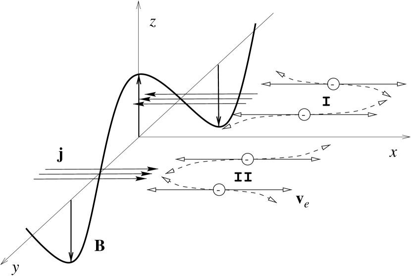
Figure 1.— Illustration of the instability. A magnetic field perturbation deflects electron motion along the $x$-axis, and results in current sheets ($j$) of opposite signs in regions I and II, which in turn amplify the perturbation. The amplified field lies in the plane perpendicular to the original electron motion.

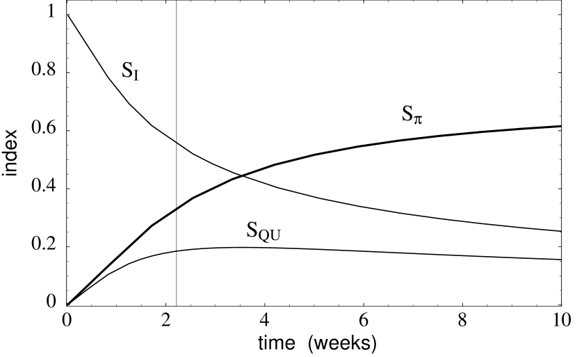
Figure 2.— Scintillation indexes of (i) intensity, $S_{I}$, (ii) the polarization signal, $S_{QU}$, and (iii) the degree of polarization, $S_{\pi}$, as functions of time for $E=10^{52}~{}{\rm ergs}$, $z_{\rm s}=1$, $n_{\rm ISM}=1~{}{\rm cm^{-3}}$, and $\pi_{\rm s}=0.72$. The thin vertical line marks the time when $\theta_{\rm s}=\theta_{0}$.

References

- Akhiezer et al. (1975) Akhiezer, A. I., et al. 1975, Plasma electrodynamics, (Pergamon: Oxford)
- Armstrong et al. (1995) Armstrong, J. W., Rickett, B. J., & Spangler, S. R. 1995, ApJ, 443, 209
- Arons (1996) Arons, J. 1996, Space Science Reviews, 75, 235
- Balbus & Hawley (1991) Balbus, S. A., & Hawley, J. F. 1991, ApJ, 376, 214
- Blandford & Narayan (1985) Blandford, R. D., & Narayan, R. 1985, MNRAS, 213, 591
- Califano et al. (1998) Califano, F., et al. 1998, Phys. Rev. E, 57, 7048
- Frail et al. (1997) Frail, D. A., et al. 1997, Nature, 389, 261
- Fried (1959) Fried, B. D. 1959, Phys. Fluids, 2, 337
- Galama et al. (1999) Galama, T. J., et al. 1999, Nature, in press; astro-ph/9903021
- Ginzburg (1989) Ginzburg, V. L. 1989, Applications of electrodynamics in theoretical physics and astrophysics, (New York: Gordon and Breach science publishers)
- Goodman (1997) Goodman, J. 1997, New Astronomy, 2, 449
- Goodman & Narayan (1985) Goodman, J., & Narayan, R. 1985, MNRAS, 214, 519
- (13) Granot, J., Piran, T., & Sari, R. 1998a, astro-ph/9806192
- (14) Granot, J., Piran, T., & Sari, R. 1998b, astro-ph/9808007
- Gruzinov & Waxman (1998) Gruzinov, A., & Waxman, E. 1998, astro-ph/9807111
- Katz (1994) Katz, J. I. 1994, ApJ, 422, 248
- Kazimura et al. (1998) Kazimura, Y. et al. 1998, ApJ, 498, L183
- Kumar, P. (1999) Private communication
- Loeb & Perna (1998) Loeb, A., & Perna, R. 1998, ApJ, 495, 597
- Mészáros, Laguna, & Rees (1993) Mészáros, P., Laguna, P., & Rees, M. J. 1993, ApJ, 415, 181
- Mészáros & Rees (1993) Mészáros, P., & Rees, M. J. 1993, ApJ, 415, 181
- Moiseev & Sagdeev (1963) Moiseev, S. S., & Sagdeev, R. Z. 1963, J. Nucl. Energy C, 5, 43
- Narayan (1999) Narayan, R. 1999, Private communication
- Narayan, Paczyński, & Piran (1992) Narayan, R., Paczyński, B., & Piran, T. 1992, ApJ, 395, L83
- Paczyński (1990) Paczyński, B. 1990, ApJ, 363, 218
- Paczyński & Xu (1994) Paczyński, B., & Xu, G. 1994, ApJ, 424, 708
- Panaitescu & Meszaros (1998) Panaitescu, A., & Meszaros, P. 1998, ApJ, 493, L31
- Pilla & Loeb (1998) Pilla, R. P., & Loeb, A. 1998, ApJ, 494, L167
- Piran (1999) Piran, T. 1999, Physics Reports, in press, astro-ph/9810256
- Rybicki & Lightman (1979) Rybicki, G. B., & Lightman, A. P. 1979, Radiative processes in astrophysics, (New York: Wiley)
- Rees & Mészáros (1994) Rees, M.J., & Mészáros, P. 1994, ApJ, 430, L93
- Sagdeev & Galeev (1969) Sagdeev, R. Z., & Galeev, A. A. 1969, Nonlinear plasma theory, (New York: Benjamin), 70
- Sari (1998) Sari, R. 1998, ApJ, 494, L49
- Sari, Narayan, & Piran (1996) Sari, R., Narayan, R., & Piran, T. 1996, ApJ, 473, 204
- (35) Sari, R., & Piran, T. 1997a, ApJ, 485, 270
- (36) ————————. 1997b, MNRAS, 287, 110
- Shemi & Piran (1990) Shemi, A., & Piran, T. 1990, ApJ, 365, L55
- Taylor et al. (1998) Taylor, G. B., et al. 1998, ApJ, 502, L115
- Thompson (1994) Thompson, C, 1994, MNRAS, 270, 480
- Vietri (1997) Vietri, M. 1997, ApJ, 478, L9
- Vreeswijk et al. (1999) Vreeswijk, P. M., et al. 1999, astro-ph/9904286
- Wallace & Epperlein (1991) Wallace, J. M., & Epperlein, E. M. 1991, Phys. Fluids B, 3, 1579
- (43) Waxman, E. 1997a, ApJ, 485, L5
- (44) —————. 1997b, ApJ, 489, L33
- (45) —————. 1997c, ApJ, 491, L19
- Waxman, et al. (1998) Waxman, E., Kulkarni, S. R., & Frail, D. A. 1998, ApJ, 497, 288
- Weibel (1959) Weibel, E. S. 1959, Phys. Rev. Lett., 2, 83
- Wijers & Galama (1998) Wijers, R. A. M. J., & Galama, T. J. 1998, ApJ, in press; astro-ph/9805341
- Wijers, Rees, & Mészáros (1997) Wijers, R. A. M. J., Rees, M. J., & Mészáros, P. 1997, MNRAS, 288, L51
- Yang et al. (1994) Yang, T.-Y., et al. 1994, Phys. Plasmas, 1, 3059
- Yoon & Davidson (1987) Yoon, P. H., & Davidson, R. C. 1987, Phys. Rev. A, 35, 2718