Magnetic fields in the early universe in the string approach to MHD

Abstract

There is a reformulation of magnetohydrodynamics in which the fundamental dynamical quantities are the positions and velocities of the lines of magnetic flux in the plasma, which turn out to obey equations of motion very much like ideal strings. We use this approach to study the evolution of a primordial magnetic field generated during the radiation-dominated era in the early Universe. Causality dictates that the field lines form a tangled random network, and the string-like equations of motion, plus the assumption of perfect reconnection, inevitably lead to a self-similar solution for the magnetic field power spectrum. We present the predicted form of the power spectrum, and discuss insights gained from the string approximation, in particular the implications for the existence or not of an inverse cascade.

I Introduction

It has been observed that many galaxies and clusters of galaxies are endowed with a magnetic field with typical strength of order $10^{-6}$ G [3]. The origin of these large scale magnetic fields is unknown. In order for magnetic fields to have this order of magnitude it is widely believed that an enormous amplification of an initial seed field must have taken place. This amplification is usually explained by dynamo theory which can enhance the magnetic field exponentially [4]. However, dynamos cannot create a magnetic field, and so in order for them to act they require a seed. At present it is not clear whether this seed field has its origin from some astrophysical mechanism after recombination, during the epoch of galaxy formation and afterwards or whether the seed field is of primordial origin, produced in the very early universe. In the latter scenario it is believed that the primordial magnetic field would have been frozen into the highly conductive plasma as the universe expanded and cooled. Because of the high conductivity diffusion would be small and magnetic flux conserved. If a magnetic field was produced in the early universe and was present at the time of recombination it may have had a significant effect on many astrophysical processes including the formation of galaxies and stars.

There are several ways of obtaining limits on cosmological magnetic fields. Limits have been obtained by Faraday rotation measurements of intergalactic fields [5, 6]. Other constraints have been obtained through the consideration of the effects of magnetic fields on primordial nucleosynthesis [8, 7, 9] and on the distortion in the microwave background due to the presence of a cosmological magnetic field [10, 11].

Even if a primordial magnetic field was to weak to be of astrophysical significance, it is still of principal interest to study cosmic magnetic fields today because they can provide direct and important information about the kind of physics that must have taken place in the early universe. There have been quite a few mechanisms proposed for ways of producing magnetic fields in the early universe. We will not discuss them here but refer to [12] for a brief review.

In this work we will not be concerned with any particular model for the generation of primordial magnetic fields. Instead we will focus on the universial problem of how a primordial field, whatever its origin, will develop as the universe evolved. In order to do this one needs to consider magnetohydrodynamics (MHD) in an expanding universe. Doing full numerical relativistic MHD simulations of the physics of the early universe is hard and requires extensive computer memory and time.

Greater dynamical range can be obtained by resorting to approximate methods. The cascade model of Ref. [13] is one such method, which is thought to reproduce well the flow of energy between wavenumbers of the full MHD equations, at the cost of a severe truncation in the number of degrees of freedom. It was found in [13] that energy was transferred from small to large scales in an inverse cascade, and that the correlation length of the initially random field increased with what looked like a small power of (conformal) time. This is pleasing if one wants to derive the galactic dynamo seed field from a primordial process, for general arguments of causality and energy conservation indicate that such an inverse cascade is actually necessary [12].

In this work we will be using a string model approach to relativistic MHD to study the evolution of cosmic magnetic fields. The connection between MHD and string dynamics have previously been studied by Semenov [14] and Olesen [15]. Our approach is simular to that of Semenov [14] but more general since we do not assume that there is a conserved particle number density. We take essentially the opposite direction of Olesen [15], in that we derive string equations from MHD and not the other way around.

Once we have reduced the MHD equations to a string model, the results can be understood in terms of the coarsening dynamics of cosmic string networks [16, 17]. The rate of increase of the network scale length $\xi$ is given by the characteristic velocity of waves on the string, in this case the Alfvén velocity, which decreases as the magnetic field decreases in strength. The string approach indicates that this decrease in strength is primarily due to reconnection on small scales: small flux loops are continually created, transferring energy away from the network of infinitely long flux lines. The transfer of energy from the large-scale field happens in a self-similar manner: the magnetic field power spectrum can be displayed as

$$|{\mathbf{B}}_{{\mathbf{k}}}|^{2}\propto\tau^{-\alpha}P(k\xi(\tau)),$$ (1)

where ${\mathbf{k}}$ is wavenumber and $\tau$ conformal time. A powerful scaling argument due to Olesen [18] shows, in the limit of ideal MHD, that $\xi\propto\tau^{2/(n+5)}$, where the initial power spectrum behaves as $k^{n}$ at low $k$. Causality dictates that $n\geq 2$ [11] (and not $n\geq 0$ as one of us [12] and another author [19] has stated). As we violate the ideal condition by allowing reconnection, it is not clear that this is the correct power of $\tau$.

This scaling law is our main result. We see no sign of a true inverse cascade, in the sense that power is not transferred from small to large scales. If anything, the transfer is from large to small, and it is only because energy is being lost faster from small scales that we see an increase in the scale length $\xi$.

II Relativistic MHD and strings

In this work we will concentrate on the ideal limit of MHD. This means that we neglect any viscous effects and treat matter as a perfect fluid. This is a good approximation at sufficiently large scales. During the radiation dominated era, which we are mainly concerned with here, the universe was a very good conductor [20, 21]. We therefore consider the $\sigma\rightarrow\infty$ limit of MHD where magnetic diffusion can be ignored and the magnetic field can be considered to be frozen into the plasma and thus conserving magnetic flux.

The starting point for ideal relativistic MHD is the energy-momentun tensor

$$T^{\mu\nu}=(\rho c^{2}+p)\frac{U^{\mu}U^{\nu}}{c^{2}}-pg^{\mu\nu}+\frac{1}{4\pi}({F^{\mu}}_{\gamma}F^{\nu\gamma}-\frac{1}{4}g^{\mu\nu}F_{\gamma\delta}F^{\gamma\delta})$$ (2)

consisting of the ideal fluid part and electromagnetic part of the energy-momentum tensor. Here $p$ is the fluid pressure, $\rho c^{2}$ is the energy density of the fluid, $U^{\mu}$ is the four-velocity of the fluid satisfying the normalisation condition $U^{\mu}U_{\mu}=c^{2}$ and $F^{\mu\nu}$ is the electromagnetic field tensor.

The evolution equations for the system are given by

$${T^{\mu\nu}}_{;\nu} = 0$$ (3)

$${F^{\mu\nu}}_{;\nu} = \frac{4\pi}{c}J^{\mu}$$ (4)

$${}^{*}\!{{F}^{\mu\nu}}_{;\nu} = 0$$ (5)

$$\sigma F^{\mu\nu}U_{\nu} = J^{\mu}-J^{\nu}U_{\nu}U^{\mu}$$ (6)

where equation (3) expresses covariant energy-momentum conservation, equations (4) and (5) are Maxwell’s equations with $J^{\mu}$ being the four-current density. In equation (5) ${}^{*}\!{{F}^{\mu\nu}}$ is the dual field tensor defined through the relation

$${}^{*}\!{{F}_{\mu\nu}}=\frac{1}{2}\epsilon_{\mu\nu\gamma\rho}F^{\mu\nu}$$ (7)

where $\epsilon_{\mu\nu\gamma\rho}$ is the Levi-Cevita symbol. Equation (6) is the relativistic version of Ohm’s law where $\sigma$ is the conductivity of the fluid, measured in the fluid rest frame.

We now repeat the derivation in Subramanian and Barrow [22] to show that the evolution equations are conformally invariant and the evolution can therefore be transformed from the expanding universe to a flat (Minkowski) spacetime. In so doing we obtain an equivalent set of equations which are easier to handle. Two metrics $g_{\mu\nu}$ and $\tilde{g}_{\mu\nu}$ are said to be conformally related to each other if $\tilde{g}_{\mu\nu}=\Omega^{2}g_{\mu\nu}$ where $\Omega$ is a non-zero differentiable function.

The flat Robertson-Walker line element has the form

$$ds^{2}=dt^{2}-a^{2}(t)d\mathbf{x}^{2}$$ (8)

where $t$ is the comoving proper time and $a(t)$ is the scale factor.

This metric describes a isotropic and homogeneous universe with zero curvature. The appearence of a hypothetical primordial magnetic field of some strength need not violate the assumption of isotropy and homogeniety because although the presence of a magnetic field will locally generate bulk motions in the fluid, if we look at sufficiently large scales isotropy and homogeniety will be regained. At large scales the magnetic field, whatever its origin, can be considered as essentially random since the correlation length of the field is bounded from above by not exceeding the causal horizon. This justifies the use of the Robertson-Walker metric.

We introduce conformal time $\tau$ defined by $d\tau=a^{-1}dt$ so that equation (8) becomes

$$ds^{2}=a^{2}(\tau)(d\tau^{2}-d\mathbf{x}^{2})$$ (9)

and hence $\eta_{\mu\nu}=\tilde{g}_{\mu\nu}=\Omega^{2}g_{\mu\nu}$ with $\Omega=a^{-1}(\tau)$.

We note that under conformal transformations the ideal energy-momentum tensor $T^{\mu\nu}$ transformation as $T^{\mu\nu}=a^{-6}\tilde{T}^{\mu\nu}$. That this is so can be seen directly from the definition of the energy-momentum tensor

$$T^{\mu\nu}=\frac{2}{\sqrt{-g}}\frac{\partial}{\partial g_{\mu\nu}}(\sqrt{-g}L_{matter})$$ (10)

The new scaled fields (denoted by tilde) obey ordinary energy-momentum conservation. To see this we note that the ideal energy-momentum tensor is traceless, $T\equiv{T^{\mu}}_{\mu}=0$, provided the perfect fluid has the equation of state $p=\frac{1}{3}\rho c^{2}$. For most of the period before decoupling, the early universe was radiation dominated and one can use the above equation of state. We have

$${T^{\mu\nu}}_{;\nu}={T^{\mu\nu}}_{,\nu}+\Gamma^{\mu}_{\nu\rho}T^{\nu\rho}+\Gamma^{\nu}_{\sigma\nu}T^{\sigma\mu}$$ (11)

Using

$$\Gamma^{\mu}_{\sigma\rho}=\frac{\dot{a}}{a}(\delta^{\mu}_{\sigma}\delta^{0}_{\rho}+\delta^{\mu}_{\rho}\delta^{0}_{\sigma}-g_{\sigma\rho}\delta^{\mu}_{0})\quad\textrm{and}\quad\Gamma^{\mu}_{\sigma\rho}=4\frac{\dot{a}}{a}(\delta^{\mu}_{\sigma})$$ (12)

we get

$${T^{\mu\nu}}_{;\nu}={T^{\mu\nu}}_{,\nu}+2\frac{\dot{a}}{a}T^{\mu 0}-\frac{\dot{a}}{a}\delta^{\mu}_{0}T+4\frac{\dot{a}}{a}T^{\mu 0}$$ (13)

But since $T=0$ then

$$(a^{-6}\tilde{T}^{\mu 0})_{,\nu}+6\frac{\dot{a}}{a}(a^{-6}\tilde{T}^{\mu 0})=({\tilde{T}}^{\mu\nu}{}_{,\nu})a^{-6}=0$$ (14)

and hence

$${\tilde{T}}^{\mu\nu}{}_{,\nu}=0$$ (15)

This means that under conformal transformations our original variables will transform to a set of new scaled variable satisfying the following relations: $\rho=a^{-4}\tilde{\rho}$, $p=a^{-4}\tilde{p}$, $U^{\mu}=a^{-1}\tilde{U}^{\mu}$, $J^{\mu}=a^{-4}\tilde{J}^{\mu}$, $F^{\mu\nu}=a^{-4}\tilde{F}^{\mu\nu}$.

Now consider Maxwell’s equation (4). Since $F^{\mu\nu}$ is anti symmetric the left hand side simplifies to

$${F^{\mu\nu}}_{;\rho}={F^{\mu\nu}}_{,\rho}+\Gamma^{\nu}_{\sigma\nu}F^{\mu\sigma}=a^{-4}{\tilde{F}}^{\mu\nu}{}_{,\rho}$$ (16)

So the equation for the scaled fields becomes

$${\tilde{F}}^{\mu\nu}{}_{,\nu}=\frac{4\pi}{c}\tilde{J}^{\mu}$$ (17)

For the four-velocity we have

$$U_{\nu}=g_{\nu\rho}U^{\rho}=a^{2}\tilde{g}_{\nu\rho}(a^{-1}\tilde{U}^{\rho})=a\tilde{U}_{\nu}$$ (18)

Hence

$$\sigma F^{\mu\nu}U_{\nu}=\sigma a^{-3}\tilde{F}^{\mu\nu}\tilde{U}_{\nu}=a^{-4}(\tilde{J}^{\mu}+\tilde{J}^{\nu}\tilde{U}_{\nu}\tilde{U}^{\mu})$$ (19)

So Ohm’s law remains invariant under conformal transformations if we define the scaled conductivity through $\sigma=\tilde{\sigma}a^{-1}$

So we arrive at the fundamental equations of relativistic MHD,

$${\tilde{T}}^{\mu\nu}{}_{,\nu} = 0$$ (20)

$${\tilde{F}}^{\mu\nu}{}_{,\nu} = \frac{4\pi}{c}\tilde{J}^{\mu}$$ (21)

$${}^{*}\!{\tilde{F}}^{\mu\nu}{}_{,\nu} = 0$$ (22)

$$\tilde{\sigma}\tilde{F}^{\mu\nu}U_{\nu} = \tilde{J}^{\mu}-\tilde{J}^{\nu}\tilde{U}_{\nu}\tilde{U}^{\mu}/c^{2}$$ (23)

From here on we drop the tilde, on the understanding that we mean scaled fields.

We will now introduce a new set of coordinates which will enable us to write the MHD equations as non-linear string equations. We define a magnetic four-vector $b^{\mu}$ through the relation

$$b^{\mu}=\,^{*}\!{F}_{\mu\nu}U^{\nu}/c$$ (24)

We also define new coordinates $x^{\prime}=(\eta,\sigma,\psi,\zeta)$ such that $\eta$ are coordinate lines of fluid elements and $\sigma$ are coordinate lines of magnetic flux. Hence $U^{\prime\mu}=(cq,0,0,0)$ and $b^{\prime\mu}=(0,\beta,0,0)$ satisfying $U^{\prime 2}=U^{2}=c^{2}$ and $b^{\prime 2}=b^{2}=-B^{2}$ respectively. Thus we have the metric tensor in the new coordinates

$\displaystyle g^{\prime}_{\mu\nu}=diag(1/q^{2},-B^{2}/\beta^{2},-h_{AB})$

where $A,B=2,3$. The new coordinate vectors are

$$\frac{\partial x^{\mu}}{\partial\eta}=\frac{U^{\mu}}{q}$$ (25)

$$\frac{\partial x^{\mu}}{\partial\sigma}=\frac{b^{\mu}}{\beta}$$ (26)

Since the introduction of these coordinates relies on the frozen in property of the plasma we will refer to them as frozen-in coordinates. In the frozen-in coordinate system we can trace the trajectories of fluid elements by simply varying the value of our time coordinate $\eta$ and keeping the values of the other coordinated fixed. Similarly, we can trace the magnetic field lines in the frozen-in system by varying the value of $\sigma$ and keeping the other three coordinates at fixed values.

The analysis of the MHD equations is usually performed in terms of the magnetic field and velocity distributions. However, in the description of MHD phenomena, the concept of a magnetic flux tube is often introduced. The reason is that it is sometimes convenient, and we gain a better physical insight, if we base the description on this concept rather on the magnetic field and velocity distributions. A magnetic flux tube is defined as the volume $V$ enclosed by a closed surface $\Sigma$ which is everywhere parallel to the ambient magnetic field vector, and two cross-sectional surface areas $S_{A}$ and $S_{B}$ at either end. The flux tube therefore consists of a bundle of magnetic field lines which enter and exit the volume through the end of surfaces $S_{A}$ and $S_{B}$.

The Cartesian coordinate system, traditionally employed in MHD does not really lend itself to an analysis of the magnetic flux tube bahaviour. The frozen-in coordinate system on the other hand, does. The frozen-in coordinates provide a coordinate system co-moving with a flux tube, and is therefore the more natural choice for the mathematical analysis of flux tube behaviour.

We now consider the equation for magnetic evolution

$${}^{*}\!{F^{\mu\nu}}_{;\nu}=0$$ (27)

Since ${}^{*}\!{F}^{\mu\nu}$ is antisymmetric the divergence is given by

$$\frac{1}{\sqrt{-g}}\partial_{\nu}(\sqrt{-g}\,^{*}\!{F^{\mu\nu}})=0$$ (28)

Using the fact that we can express the dual field tensor as

$${}^{*}\!{F}^{\mu\nu}=(b^{\mu}U^{\nu}-U^{\mu}b^{\nu})/c$$ (29)

we have

$$\frac{1}{\sqrt{-g}}\partial_{\nu}\left(\sqrt{-g}q\beta\Big{(}\frac{b^{\mu}}{\beta}\frac{U^{\nu}}{q}-\frac{U^{\mu}}{q}\frac{b^{\nu}}{\beta}\Big{)}\right)=0$$ (30)

which gives

$$q\beta\left(\Big{(}\frac{U^{\nu}}{q}\Big{)}\partial_{\nu}\Big{(}\frac{b^{\mu}}{\beta}\Big{)}-\Big{(}\frac{b^{\nu}}{\beta}\Big{)}\partial_{\nu}\Big{(}\frac{U^{\mu}}{q}\Big{)}\right)+{}$$ (32)

$${}\frac{1}{\sqrt{-g}}\left(\frac{b^{\mu}}{\beta}\partial_{\nu}(\sqrt{-g}\beta U^{\nu})-\frac{U^{\mu}}{q}\partial_{\nu}(\sqrt{-g}qb^{\nu})\right)=0$$

But first square bracket is the Lie derivative and so vanishes, giving

$$\frac{b^{\mu}}{\beta}\partial_{\nu}(\sqrt{-g}\beta U^{\nu})-\frac{U^{\mu}}{q}\partial_{\nu}(\sqrt{-g}qb^{\nu})=0$$ (33)

Thus we have

$$\partial_{\nu}(\sqrt{-g}\beta U^{\nu})=0$$ (34)

and

$$\partial_{\nu}(\sqrt{-g}qb^{\nu})=0$$ (35)

Hence in our comoving frame we get

$$\frac{\partial}{\partial\eta}(\sqrt{-g}\beta q)=\frac{\partial}{\partial\eta}(B\det(h_{AB}))=0$$ (36)

$$\frac{\partial}{\partial\sigma}(\sqrt{-g}\beta q)=\frac{\partial}{\partial\sigma}(B\det(h_{AB}))=0$$ (37)

And so we see that

$\displaystyle B\det(h_{AB})=F(\psi,\zeta)$

where $F(\psi,\zeta)$ is an arbitrary function of $\psi,\zeta$. We therefore have the freedom to choose $\det(h_{AB})$ such that $F(\psi,\zeta)=\bar{B}$ where $\bar{B}$ is a constant and so

$\displaystyle h_{AB}=\frac{\bar{B}}{B}\delta_{AB}$

which means that we can write

$\displaystyle\sqrt{-g}=\frac{\bar{B}}{\beta q}$

We now study the equations of motion, starting from the energy-momentum tensor given in equation (2). Using the above expression, equation (29), for the dual field tensor and the connection between the field tensor and its dual, equation (7), we can write the energy-momentun tensor in the following form

$$T^{\mu\nu}=\left(\rho c^{2}+p+\frac{B^{2}}{4\pi}\right)\frac{U^{\mu}U^{\nu}}{c^{2}}-\frac{b^{\mu}b^{\nu}}{4\pi}-g^{\mu\nu}\left(p+\frac{B^{2}}{8\pi}\right)$$ (38)

From energy-momentum conservation we have

$${T^{\mu\nu}}_{,\nu} = \frac{(\rho c^{2}+p+B^{2}/4\pi))}{\beta}\frac{U^{\mu}}{c}\partial_{\nu}(\beta U^{\nu})$$ (39)

$$+ \beta(U\cdot\partial)\left(\frac{(\rho c^{2}+p+B^{2}/4\pi)}{\beta}\frac{U^{\mu}}{c}\right)-$$ (41)

$${}\frac{1}{4\pi q}\partial_{\nu}(qb^{\nu})-\frac{q}{4\pi}(b\cdot\partial)\left(\frac{b^{\mu}}{q}\right)-g^{\mu\nu}P_{,\nu}=0$$

Here $P$ is the total pressure from both fluid and electromagnetic field. Note that the first and the third terms in this equation vanish. Writing this equation in our comoving reference frame we find

$$\beta q\left[\frac{\partial}{\partial\eta}\left(\Big{(}\rho c^{2}+p+\frac{B^{2}}{4\pi}\Big{)}\frac{q}{c\beta}\frac{\partial x^{\mu}}{\partial\eta}\right)-\frac{1}{4\pi}\frac{\partial}{\partial\sigma}\left(\frac{\beta}{q}\frac{\partial x^{\mu}}{\partial\sigma}\right)\right]-g^{\mu\nu}P_{,\nu}=0$$ (42)

Equation (42) is the equation of motion in the frozen-in coordinates. In the frozen-in coordinate system the MHD equation of motion reduces to a set of non-linear string equations. The behaviour of a magnetic flux tube is therefore formally analogous to that of a non-linear string. The last term of the left hand side of equation (42) take account of inhomogeneity (i.e. pressure gradients) and it describes the coupling between neighbouring flux tubes whilst moving through a non-uniform plasma medium.

To summarize, we have shown that the behaviour of a magnetic flux tube is formally analogous to that of a string and one can therefore model a magnetised plasma as a fluid composed of strings. We have relied heavily on the arguments of Semenov and Semenov and Berkinov [14], with one improvement: we have dropped their assumption that there is a conserved particle number density, which is neither necessary nor generally applicable in the early Universe. Our derivation is also complementary to that of Olesen [15], who starts from the relativistic string equations and shows that they can be interpreted as describing the motion of narrow flux tubes, providing the total pressure remains constant across the tube.

III Approximate string equations

Exploiting the freedom to change coordinates in the $\sigma,\eta$ subspace, we choose $\beta$ such that $\beta=qB$ and using this in the equation of motion (42) we have

$$\frac{1}{B}\frac{\partial}{\partial\eta}\left(\frac{c\,B}{v_{A}^{2}}\frac{\partial x^{\mu}}{\partial\eta}\right)-\frac{1}{B}\frac{\partial}{\partial\sigma}\left(B\frac{\partial x^{\mu}}{\partial\sigma}\right)-\frac{4\pi}{B^{2}q^{2}}g^{\mu\nu}P_{,\nu}=0,$$ (43)

where we have defined the relativistic Alfvén velocity as

$$v_{A}=\frac{c\,B/\sqrt{4\pi}}{\left(\rho c^{2}+p+B^{2}/4\pi\right)^{1/2}}.$$ (44)

Rearranging equation (43) we can write it as

$$\frac{1}{v_{A}}\frac{\partial}{\partial\eta}\left(\frac{1}{v_{A}}\frac{\partial x^{\mu}}{\partial\eta}\right)-\frac{\partial^{2}x^{\mu}}{\partial\sigma^{2}}=-\frac{1}{B}\frac{\partial}{\partial\eta}\left(\frac{c\,B}{v_{A}}\right)\frac{\partial x^{\mu}}{\partial\eta}+\frac{1}{B}\frac{\partial B}{\partial\sigma}\frac{\partial x^{\mu}}{\partial\sigma}+\frac{4\pi}{B^{2}q^{2}}g^{\mu\nu}P_{,\nu}$$ (45)

We now argue that for the particular situation we are interested in, it is justified to neglect the three terms on the right hand side of equation (45). The third term on the RHS of equation (45) can in general not be neglected because in many astrophysical situations pressure gradients are important. However, in the early universe the pressure from the magnetic field should be much smaller than the fluid radiation pressure and since the early universe had a very high degree of homogeniety it follows that the gradients of the total pressure are small.

The second term on the RHS of equation (45) does not have have a definite sign and so if averaged over time it will be zero. Dropping this term is equivalent to replacing $B$ by its root mean square value.

Again using the fact that the fluid radiation pressure in the early universe was much larger than the pressure from the magnetic field and remembering expression (44) for the relativistic Alfvén velocity it is seen that the first term on the right side of equation (45) is indeed small since the ratio $B/v_{A}$ is approximatly constant, thus justifying our decision to neglect it.

We now rescale the time parameter $\eta$ to $\bar{\eta}$ through the relation

$$\frac{\partial}{\partial\bar{\eta}}=\frac{c}{v_{A}(\eta)}\frac{\partial}{\partial\eta},$$ (46)

where we have called attention to the fact that the Alfvén velocity may be time-dependent. Using the above mentioned approximations and our new time parameter $\bar{\eta}$ we are left with the following equation of motion

$$\frac{1}{c^{2}}\frac{\partial^{2}x^{\mu}}{\partial\bar{\eta}^{2}}-\frac{\partial^{2}x^{\mu}}{\partial\sigma^{2}}=0.$$ (47)

We also recall that the four-dimensional orthogonality of the coordinates, and the coordinate choice enforced by $\beta=qB$, supplements this equation with constraints

$$\dot{x}\cdot x^{\prime}=0,\qquad\frac{1}{c^{2}}\dot{x}^{2}+x^{{}^{\prime}2}=0,$$ (48)

where dot (prime) denotes derivative with respect to the timelike parameter $\bar{\eta}$ $(\sigma)$.

We note that the equation (47) and constraint (48) is of exactly the same form as the equation for a Nambu-Goto string in Minkowski spacetime expressed in the conformal gauge [16, 17]. With ideal Nambu-Goto strings in Minkowski spacetime one can further take $x^{0}=c\bar{\eta}$, to obtain the system

$$\frac{1}{c^{2}}\ddot{\mathbf{x}}-\mathbf{x}^{\prime\prime} = 0,$$ (49)

$$\dot{\mathbf{x}}\cdot\mathbf{x}^{\prime} = 0$$ (50)

$$\frac{1}{c^{2}}\dot{\mathbf{x}}^{2}+\mathbf{x}^{{}^{\prime}2} = 1$$ (51)

This is not possible in general for MHD strings, for one can easily verify that

$$\dot{\mathbf{x}}\cdot\mathbf{x}^{\prime} = c\frac{\gamma^{2}}{q^{2}}\frac{{\mathbf{v}}\cdot{\mathbf{B}}}{v_{A}B},$$ (52)

$$\frac{1}{c^{2}}\dot{\mathbf{x}}^{2}+\mathbf{x}^{{}^{\prime}2} = \frac{\gamma^{2}}{q^{2}}\left(\frac{{\mathbf{v}}^{2}}{v_{A}^{2}}+\frac{({\mathbf{v}}\cdot{\mathbf{B}})^{2}}{c^{2}B^{2}}\right).$$ (53)

where $\gamma=(1-\mathbf{v}/c)^{-1/2}$ is the usual relativistic gamma factor. However, as long as ${{\mathbf{v}}\cdot{\mathbf{B}}}=0$ in the initial conditions, the first constraint is preserved by the evolution. Furthermore, we can use our remaining coordinate freedom to define $q$ by

$$q^{2}=\gamma^{2}\frac{{\mathbf{v}}^{2}}{v_{A}^{2}},$$ (54)

in which case we really do reproduce the Nambu-Goto equations. We should bear in mind however that we have made several approximations on the way, which are worth reiterating.

1. We have neglected pressure gradients.

2. We have made a kind of mean-field approximation in replacing the magnetic field by its root mean square value.

3. We have neglected the effect of the time-dependence of $B/v_{A}$.

We have argued that all this approximations are reasonable in the context of the early Universe, and find that the Nambu-Goto equations can be used to approximate a class of MHD velocity and magnetic field configurations which satisfy ${\mathbf{v}}\cdot{\mathbf{B}}=0$. They may also be a reasonable approximation to other configurations, provided we understand that the constraints are satisfied in an average sense.

IV Algorithm, simulations and results

The equation of motion (49) can be evolved using the Smith-Vilenkin algorithm [23]. The Smith-Vilenkin algorithm provides an exact discrete evolution for a string network defined on a face-centered cubic lattice and the evolution equations are

$$\mathbf{x}(\eta+\delta,\sigma)=\frac{1}{2}[\mathbf{x}(\eta,\sigma+\delta)+\mathbf{x}(\eta,\sigma-\delta)]+\mathbf{v}(\eta,\sigma)\delta$$ (55)

$$\mathbf{v}(\eta+\delta,\sigma)=\frac{1}{2}[\mathbf{v}(\eta,\sigma+\delta)+\mathbf{v}(\eta,\sigma-\delta))]+\frac{1}{4\delta}[\mathbf{x}(\eta,\sigma+2\delta)-2\mathbf{x}(\eta,\sigma)+\mathbf{x}(\eta,\sigma-2\delta)]$$ (56)

By using a leap-frog method, updating the positions and velocities at alternate timesteps, the above equations allow us to calculate the exact future evolution of $\mathbf{x}$ and $\mathbf{v}$ from some appropriately choosen initial conditions.

Initial string configurations are generated by a method due to Vachaspati and Vilenkin [24]. They considered string formation in a global $U(1)$- model. The $U(1)$-manifold is discretized by allowing the phase to take only three possible values. These values are then placed randomly on the sites of the cubic lattice. As we go around the face of a cube in real space, the phase descibes a certain trajectory in the group space. A string passes through the face of a cube if that trajectory has a non-zero winding number. With this method the string segments join up to form either closed loops or else open strings which intersect the boundaries of the cubic lattice. The shape of the strings will be Brownian with step size corresponding to the cell size of the lattice.

We have seen how relativistic MHD under the approximations discussed above can be described in terms of magnetic flux tubes satisfying the Nambu-Goto equations of motion. In order to represent the continuous distribution of magnetic flux by a network of string, we gather together a flux $\Phi$ into ideal Nambu-Goto strings at positions $X^{i}(\bar{\eta},\sigma)$, with [15]

$$B^{i}(\tau,\mathbf{x})=\Phi\int d\sigma\frac{\partial X^{i}(\bar{\eta},\sigma)}{\partial\sigma}\delta^{3}\left(\mathbf{x}-\mathbf{X}(\bar{\eta},\sigma)\right)$$ (57)

A few words need to be said about reconnection. In real fluids, magnetic flux tubes interact and reconnections take place when the field lines cross each other. In ideal MHD there are no dissipative or viscous effects. Physical reconnection between field lines cannot take place without resistive effects and therefore the topology of the magnetic field lines is frozen in the fluid and does not change with time.

Reconnection, which is a local process, is difficult to describe and the details are not well understood. The efficiency of reconnection is not known and neither is how this process depend on the local geometry involved, like the relative inclination of the flux tubes. To answer this question, one has to go to numerical solutions of the underlying theory, that is MHD.

In order to allow for reconnection to take place in our simulations we will take a more simple approach to reconnection. In our model strings are allowed to reconnect only if they pass through the same lattice point. When two strings meet, they intercommute with a probability $P$ and in this work we put $P=1$. Reconnection here take place instantaneously between the discrete evolution time steps. This is physically reasonable since the reconnection timescale is small compared with the evolution of the system.

We use a simple estimate for the characteristic length scale $\xi$ which is defined by

$$\xi^{2}=V/L,$$ (58)

where $V$ is the volume of the lattice and $L$ is the total length of string in the box, excluding small loops. In the Smith-Vilenkin algorithm it is in fact possible to have a loop of zero spatial extent, occupying just one lattice point, which travels at the wave velocity. If such a loop is formed it does not contribute to the magnetic field, and we do not count it in the calculation of the total length. It is a well-known feature of Nambu-Goto simulations that nearly all the string ends up in this kind of loop [16, 17]. In the MHD context we should probably not regard these loops as representing magnetic field lines at all: the energy is probably being dissipated in a very small-scale reconnection process. In any case, the fact that loops are generically produced so small underlines the fact that strings are very efficient at transferring power from large to small scales.

We have studied simulations of the evolution of the magnetic field on lattices with sizes $(128\delta)^{3}$ and $(256\delta)^{3}$, using a code originally developed by Sakellariadou [25], which implements both the Vachaspati-Vilenkin algorithm for the initial conditions and the Smith-Vilenkin alorithm for the evolution. Periodic boundary conditions were used in all simulations and the evolution time were resticted to less than half the box size, since after this time causal influences have had time to propagate around the box.

Having a representation for the magnetic field in real space we use a three dimensional Fast Fourier Transform algorithm to get a Fourier mode representation. The power spectrum for the magnetic field $|\mathbf{B}_{k}|^{2}$ can then be calculated at every time step by averaging over the amplitudes of all Fourier modes with a wave number between $k$ and $k+2\pi/\delta$.

Previously it has been shown that networks of cosmic strings, modelled as Nambu- Goto strings in Minkowski spacetime tend towords a scaling regime [26]. This means that the characteristic length scale of the network grows as $\sim c\,t$ where $t$ is Minkowski time. The characteristic length scale for a primordial magnetic field $\xi$ does not grow with the horizon. Instead we expect the magnetic field to grow as $\sim c\,\bar{\eta}$.

It is interesting to see if the magnetic field power spectra show scaling behaviour. In order to investigate this we express the power spectrum in terms of a scaling function $P$ which is defined through the following expression

$$|B(k,\bar{\eta})|^{2}=V\frac{\Phi^{2}P(k\xi)}{\xi}.$$ (59)

Here $V$ is the volume of the box and its appearance is just a normalisation convention. This form for the scaling function ensures that that the fluctuations obey the scaling law

$$B^{2}=\int\frac{d^{3}k}{(2\pi)^{3}}|B_{k}|^{2}\propto\xi^{-4}\Phi^{2}$$ (60)

which is consistent with our picture of a coherent flux $\Phi$ in a region of size $\xi$.

Figure 1 shows the chacteristic length scale of the magnetic field versus $c\,\bar{\eta}$ for a typical ensemble. The measured scaling function $P(k\xi)$ is displayed in Figure 2. The data was taken from 12 runs on a $(256\delta)^{3}$ lattice, for values of $c\,\bar{\eta}$ between $40-60$. It is seen that the power spectrum of the magnetic field does reach a scaling regime. This means that the evolution of the network will be self-simular with respect to $c\,\bar{\eta}$.

It is clear that the network does exhibit the property of scaling, with $\xi=x\!_{*}\cdot c\,\bar{\eta}$. The scaling amplitude $x\!_{*}$ can be obtained by looking at the ratio $\xi/\bar{\eta}$ towards the end of the simulation and it is roughly $x\!_{*}\simeq 0.3$ (see [26] for a more accurate determination). Thus we can write

$$\xi=x\!_{*}\cdot c\,\bar{\eta}=x\!_{*}\int v_{A}(\eta)d\eta.$$ (61)

Unfortunately, we do not yet know how $v_{A}$ depends on the time parameter $\eta$ or the conformal time $\tau$. The Alfvén velocity $v_{A}$ depends on $B$, which in turn depends on $\Phi$ and $\xi$ through (59). All we can infer from the information at hand is a consistency relation: if $\xi\propto\eta^{r}$ and $\Phi\propto\eta^{s}$, then $3r=s+1$.

The extra information we need comes from the covariance of ideal MHD under the scale transformation [18]

$${\mathbf{x}}\to l{\mathbf{x}},\quad\tau\to l^{1-h}\tau,\quad{\mathbf{v}}\to l^{h}{\mathbf{v}},\quad{\mathbf{B}}\to l^{h}{\mathbf{B}},$$ (62)

where $h$ is arbitrary. One can show that under this transformation,

$$V^{-1}|\mathbf{B}_{k}|^{2}\to l^{3+h}V^{-1}|\mathbf{B}_{k}|^{2}.$$ (63)

If we define a function $\Lambda(k,\tau)$ by

$$V^{-1}|\mathbf{B}_{k}|^{2}=\tau^{(3+h)/(1-h)}\Lambda(k,\tau),$$ (64)

then we see that under the same transformation

$$\Lambda(k,\tau)\to\Lambda(k/l,\tau l^{1-h})=\Lambda(k,\tau),$$ (65)

from which we immediately infer that

$$\Lambda(k,\tau)=\Lambda(k\tau^{1/(1-h)}).$$ (66)

Furthermore, if $|\mathbf{B}_{k}|^{2}$ behaves as $k^{n}$ as $k\to 0$, we have

$$|\mathbf{B}_{k}|^{2}\propto\tau^{(3+h+n)/(1-h)}k^{n}$$ (67)

in that limit. It is often assumed that the large-scale power is not affected by small-scale processes [18, 19], in which case $h=-n-3$, and we find the scaling laws (derived by the same authors)

$$\xi\propto\tau^{2/(n+5)},\qquad\Phi\propto\tau^{(1-n)/(n+5)}.$$ (68)

In the early universe individual particles move with relativistic velocities. However, we expect that the bulk velocity of the fluid $v$ to be non-relativistic. Hence

$$U^{0}=qc\frac{\partial\tau}{\partial\eta}\simeq c,$$ (69)

and given (54) we see that, on average,

$$\eta=\sqrt{\langle{\dot{\mathbf{x}}^{2}}\rangle}\tau/v_{A},$$ (70)

where $\langle{\dot{\mathbf{x}}^{2}}\rangle$ is the mean square string velocity. Simulations give this to be $0.36$ [26].

V Conclusions

We have seen how the relativistic MHD equations, with a few reasonable assumptions, may be recast as string-like equations for the motion of the flux lines. This allows us enormous gains in dynamic range in the simulation of a random magnetic field in the early Universe, without being forced to the ideal limit, for we incorporate diffusivity by allowing reconnections between the strings.

The result is that we can understand the evolution of magnetic fields in terms of the evolution of a network of strings, and we find that the power spectrum quickly evolves to a self-similar or scale-invariant form, with scale length $\xi$ increasing in time. What this power law is we are unable to say: ideal MHD predicts $\xi\propto\tau^{2/(n+5)}$, where $n$ is the low $k$ exponent of the power spectrum, but as we have departed from ideality by allowing reconnection, we cannot make a prediction.

The increase in scale length comes about by the strings straightening at the Alfvén velocity, while forming very small loops which can dissipate energy quickly. This is the new feature that the string formulation brings to light: strings transfer energy from large to small scales in an extremely efficient manner. Thus, although the scale length increases, it is because power is preferentially lost from small scales. Whether it is fair to call this an inverse cascade is a matter of terminology. What is clear is that the dynamics predicted by the string model of MHD is certainly not of the right kind to produce seeds for the galactic dynamo from magnetic fields created in the very early Universe.

There are of course many places where this line of argument is vulnerable. The model makes approximations which we have tried to highlight. Furthermore, our string simulations use special string configurations to make gains in computational efficiency: the strings lie on a cubic lattice to start with, and one may be suspicious that this may introduce some artifice into the dynamics. However, the propensity of a string network to scale is firmly believed, so we are confident that the magnetic field power spectrum will also scale. What is probably not well approximated is the actual form of the power spectrum, which betrays the particularly string-like feature of a $k^{-1}$ tail, due to the fact that all the flux is held to be concentrated in a narrow tube. Furthermore, the string model may be deficient in its description of helicity, which is known to be extremely important in the development of true inverse cascades [27, 28, 29]. The helicity is represented by the linking number of the strings, but we are not able to incorporate a local contribution induced, for example, by twisted tubes of flux. It may well be that we are missing some very important dynamics here. We clearly need to check our results against a non-ideal MHD code, to see if the predicted self-similar dynamics emerges, and also to find the correct power law for the scale length. This project is currently in hand.

We are extremely grateful to Mairi Sakellariadou for the use of her Minkowski space string code. We have also benefited from conversations with Axel Brandenburg, Carlo Barenghi, Richard Rijnbeek and Vladimir Semenov. MH is supported by PPARC grant no. GR/L56305. MC is supported by Centrala Studienämden (CSN).

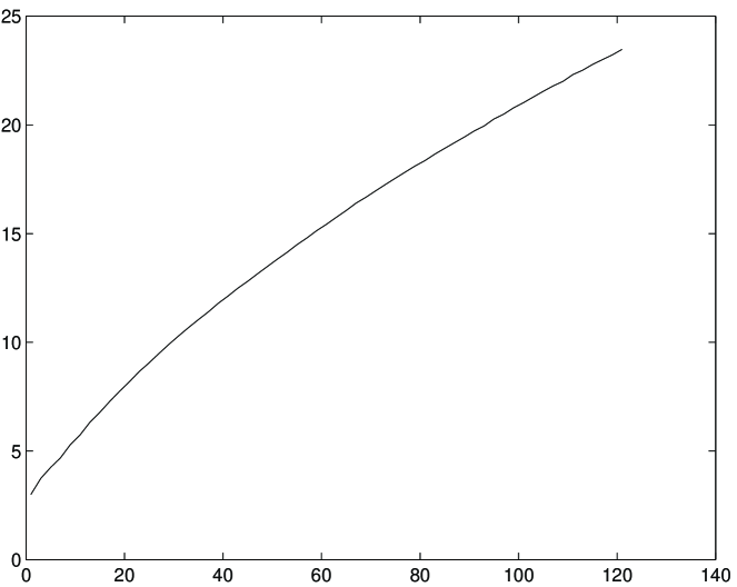
FIG. 1.: Correlation length $\xi$ versus $c\bar{\eta}$

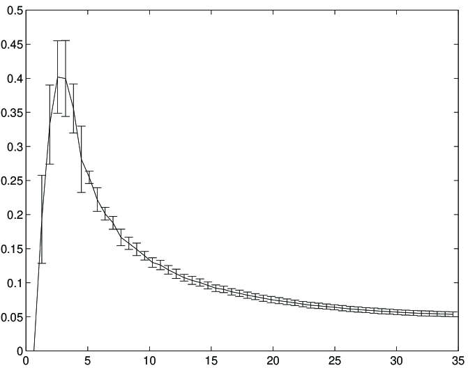
FIG. 2.: Scaling function $P(k\xi)$ versus $k\xi$

REFERENCES

- [1] Electronic address: m.christensson@sussex.ac.uk
- [2] Electronic address: m.b.hindmarsh@sussex.ac.uk
- [3] P.P. Kronberg, Rep. Prog. Phys. 57, 325 (1994).
- [4] Ya.B. Zeldovich, A.A. Ruzmaikin and D.D. Sokoloff, Magnetic Fields in Astrophysics (McGraw-Hill, New York, 1980); A.A. Ruzmaikin, A.A.Shukurov and D.D. Sokoloff, Magnetic Fields in Galaxies (Kluwer, Dordrecht, 1988).
- [5] J.P. Vallee, Astrophys. J. 360, 1 (1990).
- [6] P. Blasi, S. Burles and A.V. Olinto, astro-ph/9812487.
- [7] D. Grasso and H.R. Rubinstein, Phys. Lett. B379, 73 (1996); D. Grasso and H.R. Rubinstein, Astropart. Phys. 3, 95 (1995).
- [8] P.J. Kernan, G.D. Starkman and T. Vachaspati, Phys.Rev. D54, 7207 (1996); P.J. Kernan, G.D. Starkman and T. Vachaspati, Phys.Rev. D56, 3766 (1997).
- [9] B. Cheng, A.V. Olinto, D. Schramm and J.W. Truran, Phys. Rev. D54, 4714 (1996); B. Cheng, D. Schramm and J.W. Truran, Phys. Rev. D49, 5006 (1994).
- [10] J.D. Barrow, P.G. Ferreira and J. Silk, Phys. Rev. Lett 78, 3610 (1997); J.D. Barrow, Phys. Rev. D55, 7451 (1997).
- [11] R. Durrer, T. Kahniasvili and A. Yates, astro-ph/9807089.
- [12] M.Hindmarsh and A. Everett, Phys. Rev. D58, 103505 (1998).
- [13] A. Brandenburg, K. Enqvist, P. Olesen, Phys. Rev. D54, 1291 (1997).
- [14] V.S. Semenov in The Solar Wind-Magnetospere System, edited by H.K. Biernat, G.A. Bachmaier, S.J. Bauer and R.P. Rijnbeek (Austrian Academy of Sciences Press, 1994); V.S. Semenov and L.V. Bernikov, Sov. Phys. JETP 71 (5), 911 (1990).
- [15] P. Olesen, Phys. Lett. B366, 117 (1996).
- [16] A. Vilenkin and P. Shellard, Cosmic strings and other topological defects (Cambridge University Press, 1994).
- [17] M. B. Hindmarsh and T. W. B. Kibble, Rept. Prog. Phys. 58, 477 (1995).
- [18] P. Olesen, Phys. Lett. B398, 321 (1997).
- [19] D.T. Son, Phys. Rev. D59, 063005 (1999).
- [20] M.S. Turner and L.M. Widrow, Phys. Rev. D30, 2743 (1988).
- [21] J. Ahonen and K. Enqvist, Phys. Lett. B382, 40 (1996).
- [22] K. Subramanian and J.D. Barrow, Phys. Rev. D58, 083502 (1998).
- [23] A.G. Smith and A. Vilenkin, Phys. Rev. D36, 990 (1987).
- [24] T. Vachaspati and A. Vilenkin, Phys. Rev. D30, 2036 (1984).
- [25] M. Sakellariadou and A. Vilenkin Phys Rev D37, 885 (1988)
- [26] G. Vincent, M. Hindmarsh and M. Sakellariadou, Phys. Rev. D56, 637 (1998).
- [27] A. Pouquet, U. Frisch, J. Leorat, J. Fluid. Mech. 77, 321 (1976); M. Meneguzzi, U. Frisch, A. Pouquet, Phys. Rev. Lett. 47, 1060 (1981).
- [28] J.M. Cornwall, Phys.Rev. D56, 6146 (1997)
- [29] G.B. Field and S.M. Carroll, astro-ph/9811206