Distances in Inhomogeneous Cosmological Models

1 Introduction

In optical relations among observed quantities, distances such as the luminosity distance and the angular diameter distances play an important role. They are clearly defined in the homogeneous Friedmann-Lemaitre-Robertson-Walker model (Weinberg,[1] Schneider et al.[2]) owing to the simple nature of light propagation in this case. In inhomogeneous universes, however, their behavior is complicated, due to gravitational lens effect which implies that light rays are deflected gravitationally by an inhomogeneous matter distribution. On the other hand, we also use distances to interpret the structure of gravitationally lensed systems.

To correctly treat distances in inhomogeneous universes, it is necessary first to have a reasonable formulation for the dynamics describing local matter motion and optics and clarify the validity condition of the formulation. A set of fluid dynamical equations and the Poisson equation in the cosmological Newtonian approximation was introduced and discussed by Nariai[3] and Irvine[4] under the conditions

$$|\mathchar 28936\relax|\ll 1,\ (v/c)^{2}\ll 1,\ L/L_{H}\ll 1,$$ (1.1)

where $\mathchar 28936\relax,\ v,L$ and $L_{H}$ are the Newtonian gravitational potential, matter velocity, the characteristic size of inhomogeneities and the horizon size $\approx ct$, respectively, and the spacetime is expressed as

$$ds^{2}=-(1+2\mathchar 28936\relax)c^{2}dt^{2}+(1-2\mathchar 28936\relax)a^{2}(t)[d\chi^{2}+\sigma^{2}(\chi)d\mathchar 28938\relax^{2}],$$ (1.2)

where $a(t)$ is the scale-factor, $\sigma(\chi)=\sin\chi,\chi,\sinh\chi$ for the background curvature $k=1,0,-1$, respectively, and $d\mathchar 28938\relax^{2}=d\theta^{2}+\sin^{2}\theta\varphi^{2}$. The above fluid dynamical equations can describe the nonlinear local motion, while the gravitational field is linear with respect to $\mathchar 28936\relax$. The extension of the above cosmological Newtonian treatment to a post-Newtonian treatment was performed by Futamase,[5] Tomita[6] and Shibata and Asada.[7] Futamase showed that the condition

$$\epsilon^{2}/\kappa\ll 1\quad(\epsilon^{2}\sim\mathchar 28936\relax\ {\rm and}\ \kappa\sim L/L_{H})$$ (1.3)

is necessary for the higher-order expansion to be possible and formulated the spatial averaging and the back-reaction to the background. Moreover, Futamase and Sasaki[8] investigated the validity of light propagation in the cosmological Newtonian iterative approximation and discussed the distance problem.

In an empty region as the limiting inhomogeneous case, distances exhibit behavior very different from those in homogeneous models (the Friedmann distances). In the special case without tidal shear from surrounding regions, the so-called Dyer-Roeder angular diameter distance was derived by Zel’dovich,[9] Dashevskii and Slysh[10] and Dyer and Roeder.[11]${}^{\hbox{\,-}}$[12] In a non-empty region with a constant matter density $\rho_{m}$ but no tidal shear, we have the generalized Dyer-Roeder distance with the clumpiness (or smoothing) parameter $\alpha$, which is defined as

$$\rho_{m}/\rho_{\rm F}=\alpha={\rm const}$$ (1.4)

for the Friedmann density $\rho_{\rm F}$. The observational results derived from the optical relations depend on whether we use the Friedmann distances or the Dyer-Roeder distance. Quantitative estimates for these difference and the effect of the cosmological constant have been studied by Fukugita et al.[13] and Asada.[14] On the other hand, it is important to determine what distances are most applicable and what value of the above parameter $\alpha$ is best, in realistic inhomogeneous models. Kasai et al.[15] and Watanabe and Tomita[16] numerically calculated the frequency distribution for generalized distances in simple models in which particles are distributed randomly. Recently, Tomita[17] derived this distribution in more realistic inhomogeneous models generated using the $N$-body simulation with the CDM spectrum. The general result is that the average value of $\alpha$ is nearly 1 and its dispersion decreases with the increase of the redshift $z$, though it is $\sim 1$ for $z=0.5$.

Another interesting topic is that involving the role of the shear term and the Ricci and Weyl focusing terms (in the optical scalar equation[18]) in the behavior of distances. To this time, the shear effect has been discussed by Weinberg,[19] Watanabe et al.,[20] Watanabe and Sasaki,[21] and Nakamura,[22] and its focusing effect has recently been studied numerically by Hamana using a Monte Carlo simulation, taking into account small-scale inhomogeneities.

In this review paper, basic optical relations and the definition of distances are first given in §2, the lensing relations in the generalized Dyer-Roeder distance are derived in §3 (by Asada), the statistical behavior of distances analyzed in numerical simulation is described in §4 (by Tomita), and the shear and focusing effects are discussed in §5 (by Hamana).

2 Optical scalars and the definition of distances

2.1 Geometry of ray bundles

Rays are expressed as $x^{\mu}=x^{\mu}(y^{i},v)$, where $v$ is an affine parameter. For each ray, the $y^{i}$ have constant values ($C^{i}$). The wave vector $k^{\mu}=\partial x^{\mu}/\partial v$ satisfies the null condition and null-geodesic equation

$$k^{\alpha}k_{\alpha}=0,\quad{k^{\alpha}}_{;\beta}k^{\beta}=0.$$ (2.1)

For two rays with $y^{i}=C^{i}$ and $y^{i}=C^{i}+\delta C^{i}$, the connection vector is

$$\delta x^{\mu}=({\partial x^{\mu}/\partial y^{i}})\delta C^{i}.$$ (2.2)

If we define a dot differentiation by $(m^{\alpha})^{\cdot}={m^{\alpha}}_{;\beta}k^{\beta}$  for an arbitrary vector $m^{\mu}$, we obtain from Eq. (2.2)

$$(\delta x^{\alpha})^{\cdot}={k^{\alpha}}_{;\beta}\delta x^{\beta},$$ (2.3)

and then (Jordan et al.,[23] Sachs[18])

$$(k_{\alpha}\delta x^{\alpha})^{\cdot}=0.$$ (2.4)

Now let us consider the situation in which on a screen (at a point P_o) an observer sees the shadow formed by a source object (at a point P_s). The connection vector $\delta_{\bot}x^{\alpha}$ vertical to $u^{\alpha}$ and $k^{\alpha}$ at the point P_s is

$$\delta_{\bot}x^{\alpha}=h^{\alpha}_{\beta}\delta x^{\beta},$$ (2.5)

where

$$h^{\alpha}_{\beta}=\delta^{\alpha}_{\beta}-{k^{\alpha}k_{\beta}\over(k^{\gamma}k_{\gamma})^{2}}-{k^{\alpha}u_{\beta}+u^{\alpha}k_{\beta}\over k^{\gamma}u_{\gamma}}.$$ (2.6)

The $h^{\alpha}_{\beta}$ satisfy the relation

$$h^{\alpha}_{\beta}h^{\beta}_{\gamma}=h^{\alpha}_{\beta},\ h^{\alpha}_{\beta}u^{\beta}=h^{\alpha}_{\beta}k^{\beta}=0\ {\rm and}\ h^{\alpha}_{\alpha}=2.$$ (2.7)

If $\bar{\delta}x^{\alpha}$ is the vector obtained by parallel-transporting $\delta_{\bot}x^{\alpha}$ from P_s along the ray, we have

$$\bar{\delta}x^{\alpha}=\delta_{\bot}x^{\alpha}+\int(\delta_{\bot}x^{\alpha})^{\cdot}dv,$$ (2.8)

and the connection vector $\bar{\delta}_{\bot}x^{\alpha}$ vertical to $u^{\alpha}$ and $k^{\alpha}$ at the point P_o is

$$\bar{\delta x^{\alpha}}=h^{\alpha}_{\beta}\bar{\delta}x^{\beta}=\delta_{\bot}x^{\alpha}+\int h^{\alpha}_{\beta}(\delta_{\bot}x^{\beta})^{\cdot}dv.$$ (2.9)

The length $\delta l$ and the angle $\alpha_{12}$ are expressed as follows using the connection vector in the plane vertical to $k^{\alpha}$ and the screen velocity $\bar{u}^{\alpha}$ :

$$\delta l=(g_{\alpha\beta}\bar{\delta}x^{\alpha}\bar{\delta}x^{\beta})^{1/2},\ \cos\alpha_{12}=[(\bar{\delta}x^{\alpha})_{1}(\bar{\delta}x^{\beta})_{2}]/[(\delta l)_{1}(\delta l)_{2}].$$ (2.10)

Here $\bar{u}^{\alpha}$ is parallel-transformed along the ray from $u^{\alpha}$ at P_s.

2.2 Optical scalars

Using Eqs.(2.3) and (2.4) we obtain

$$(\delta_{\bot}x^{\alpha})^{\cdot}=A^{\alpha}_{\beta}\delta_{\bot}x^{\beta},$$ (2.11)

where

$$A_{\alpha\beta}=h^{\gamma}_{\alpha}h^{\lambda}_{\beta}k_{\gamma;\lambda}.$$ (2.12)

The tensor $A_{\alpha\beta}$ can be uniquely split as

$$A_{\alpha\beta} = A_{[\alpha\beta]}+\theta h_{\alpha\beta}+\sigma_{\alpha\beta},$$ (2.13)

$$\omega = \Bigl{[}{1\over 2}A_{[\alpha\beta]}A^{\alpha\beta}\Bigr{]}^{1\over 2}=\Bigl{[}{1\over 2}k_{[\alpha;\beta]}k^{\alpha;\beta}\Bigr{]}^{1\over 2},$$ (2.14)

$$\theta = {1\over 2}A^{\gamma}_{\gamma}={1\over 2}k^{\gamma}_{;\gamma},\quad\sigma_{\alpha\beta}=A_{(\alpha\beta)}-{1\over 2}A^{\gamma}_{\gamma}h_{\alpha\beta},$$ (2.15)

$$\sigma = \Bigl{(}{1\over 2}\sigma_{\alpha\beta}\sigma^{\alpha\beta}\Bigr{)}^{1\over 2}=\Bigl{\{}{1\over 2}[k_{(\alpha\beta)}k^{\alpha\beta}-{1\over 2}(k^{\gamma}_{;\gamma})^{2}]\Bigr{\}}^{1\over 2},$$ (2.16)

where $\theta,\sigma$ and $\omega$ are optical scalars representing the expansion, shear and rotation, respectively, of ray bundles. In geometric optics which we assume in the following, the rotation vanishes, because $k^{\mu}$ is a gradient vector. By the transformation of $v$, $\theta,\sigma$ and $\omega$ transform, but $\theta dv,\sigma dv$ and $\omega dv$ are invariant (Jordan et al.,[23] Sachs[18]).

The evolution equations for $\theta$ and $\sigma$ are

$${d\theta\over dv}={1\over 2}k^{\mu}_{;\mu\nu}k^{\nu}=-{1\over 2}{\cal R}-(\theta^{2}+\sigma^{2}),$$ (2.17)

$${d\sigma\over dv}=-{\cal C}-2\theta\sigma,$$ (2.18)

where ${\cal R}\equiv R_{\mu\nu}k^{\mu}k^{\nu}$, and ${\cal C}$ is expressed in terms of the Weyl tensor as ${\cal C}\equiv C_{\alpha\beta\gamma\lambda}k^{\alpha}k^{\gamma}\bar{t}^{\beta}\bar{t}^{\lambda}$, with $t^{\alpha}$ a complex null vector satisfying $t^{\alpha}t_{\alpha}=k^{\alpha}t_{\alpha}=0,\bar{t}^{\alpha}\bar{t}_{\alpha}=1$. As can be seen from Eqs. (2.17) and (2.18) there two terms causing the focusing of ray bundles. One is the Ricci focusing term ${\cal R}$, proportional to the matter density, and the other is the Weyl focusing term ${\cal C}$, connected with the shear.

2.3 Definition of distances

The length of the shadow of the interval between two rays in the observer plane is given by

$$(dl)^{2}=g_{\alpha\beta}\bar{\delta}_{\bot}x^{\alpha}\bar{\delta}_{\bot}x^{\beta}.$$ (2.19)

Then we have

$${d(\delta l)\over\delta l}=A_{\alpha\beta}e^{\alpha}e^{\beta}dv=(\theta+\sigma_{\alpha\beta}e^{\alpha}e^{\beta})dv,$$ (2.20)

where $e^{\alpha}\equiv\delta_{\bot}x^{\alpha}/\delta l$ and $g_{\alpha\beta}e^{\alpha}e^{\beta}=1$. Next, let us consider the area of the cross-section of a ray bundle given by

$$\delta A={1\over 2}{\int_{0}}^{2\pi}(\delta l)^{2}d\alpha.$$ (2.21)

If the deviation of the cross-section from a circle is small, we obtain

$$d(\delta A)=(\delta A)^{\cdot}dv=dv\delta A{\int_{0}}^{2\pi}{d(\delta l)\over\delta l}d\alpha$$ (2.22)

or

$${d(\delta A)\over\delta A}=2\theta dv,$$ (2.23)

because ${\int_{0}}^{2\pi}\sigma_{\alpha\beta}e^{\alpha}e^{\beta}d\alpha$ vanishes.

Here we define two kinds of angular diameter distances (the linear angular diameter distance $D_{\rm lA}$ and the area angular diameter distance $D_{\rm aA}$) proportional to $\delta l$ and $(\delta A)^{1/2}$, respectively, as

$${dD_{\rm lA}\over dv}=(\theta+\sigma_{\alpha\beta}e^{\alpha}e^{\beta})D_{\rm lA},$$ (2.24)

$${dD_{\rm aA}\over dv}=\theta D_{\rm aA},$$ (2.25)

where we consider ray bundles with $\theta=\infty$ at the observer point P_o. In the case of no shear, $D_{\rm lA}$ and $D_{\rm aA}$ are equal, but generally they are different. Their average values are equal if the term $\sigma_{\alpha\beta}e^{\alpha}e^{\beta}$ is cancelled out in the averaging process. In the situation that $\theta=\infty$ at the source’s point P_s, we obtain the luminosity distance $D_{\rm L}$ satisfying

$${dD_{\rm L}\over dv}=\theta D_{\rm L}.$$ (2.26)

The relation between $D_{\rm aA}$ and $D_{\rm L}$ is proved to be

$$D_{\rm L}=(1+z)^{2}D_{\rm aA}$$ (2.27)

by Etheringen,[24] where $z$ is the redshift given by the relation $1+z=(u^{\alpha}k_{\alpha})_{\rm source}\\ /(u^{\alpha}k_{\alpha})_{\rm observer}$.

The solutions of Eqs. (2.24) and (2.25) are generally complicated, but they can easily be obtained in the special case in which (1) the density is spatially constant, (2) there is no shear, and (3) the affine parameter in the Friedman background can be used. From Eqs. (2.17) and (2.25) we obtain

$${d^{2}D_{\rm A}\over dv^{2}}=-{1\over 2}{\cal R}D_{\rm A},$$ (2.28)

where $D_{\rm A}=D_{\rm lA}=D_{\rm aA}$, ${\cal R}=8\pi G\alpha\rho/a^{2}(t)=3(1+z)^{5}\alpha\mathchar 28938\relax_{0}$, $\mathchar 28938\relax_{0}$ is the total density parameter, and $\alpha$ is the smoothing (clumpiness) parameter. The affine parameter $v$ is related to $z$ as

$${dz\over dv}=(1+z)^{2}[(1+\mathchar 28938\relax_{0}z)(1+z)^{2}-\lambda_{0}z(2+z)]^{1/2},$$ (2.29)

where $\lambda_{0}$ is the normalized cosmological constant. The boundary condition for $D_{\rm A}$ at epoch $z=z_{1}$ is

$$D_{\rm A}=0,\quad{dD_{\rm A}\over dz}=c(dt/dz)_{z=z_{1}}={c\over H_{0}}{a(z_{1})\over a_{0}}.$$ (2.30)

The solution of Eq. (2.29) is called the Friedmann distance for $\alpha=1$, the Dyer-Roeder distance for $\alpha=0$, and the generalized Dyer-Roeder distance for arbitrary $\alpha$.

For the analyses of cosmological lens systems, we often use the lens equation

$$\mbox{\boldmath$\beta$}=\mbox{\boldmath$\theta$}-4G{D_{OL}D_{LS}\over D_{OS}}{\partial\over\partial\mbox{\boldmath$\theta$}}\int d^{2}\theta^{\prime}\mathchar 28934\relax(\theta^{\prime})\ln{|\theta-\theta^{\prime}|\over\theta_{c}},$$ (2.31)

where $\beta$ and $\theta$ are the angular position vectors (as seen by the observer) of the image and source, respectively, relative to the lens, $\mathchar 28934\relax(\theta^{\prime})$ is the surface mass density of the lens on the lens plane, $\theta_{c}$ is an arbitrary constant angle, and $D_{OL},D_{OS}$ and $D_{LS}$ are the angular distances between the lens and the observer, the source and the observer, and the lens and the source, respectively. This equation has so far been derived only from intuitive geometrical considerations with use of the thin lens approximation, but it is not clear what distances should be used. In order to derive the lens equation from cosmological equations of light propagation, Sasaki[25] used the equation of geodesic deviation. It is obtained from Eq. (2.3) for the connection vector:

$$(\delta x^{\mu})^{\cdot\cdot}=-R^{\mu}_{\nu\alpha\beta}k^{\nu}k^{\beta}\delta x^{\alpha}.$$ (2.32)

He solved this equation in the case of an ideal light path, which is separated into three regions: the homogeneous, shearless region I (between the observer and the lens object), the region II including the lens object, and the homogeneous, shearless region III (between the lens object and the source). The light path in regions I and III is expressed by the generalized Dyer-Roeder distance, and the deflection of light rays in region III is determined using the thin lens approximation. The resulting lens equation reduces to the usual one with the generalized Dyer-Roeder distances. In the case that in the regions I and III there are inhomogeneous matter distributions and the shear effect is not negligible, however, the usual expression of the lens equation cannot be used, as was shown by Sasaki.[25]

In the multi-lens-plane method,[2][26]${}^{\hbox{\,-}}$[27] inhomogeneities as lens objects are assumed to be only in the lens planes, and hence the use of the lens equation in this method is consistent with the above assumption that the regions I and III are homogeneous and shearless. However the neglection of gravitational forces due to the difference of the projected matter distribution from the real distribution may be comparable with the neglection of weak forces from distant matter distribution.

3 Distances and lensing relations

3.1 Observation and distances in gravitational lensing

There are some methods to determine cosmological parameters by using gravitational lenses. [29, 30, 31, 32, 33, 34, 13, 2] Most of them concern the following three typical observational quantities: (1) the bending angle, (2) the lensing statistics and (3) the time delay. It is of great importance to clarify the determination of cosmological parameters through their observations in the realistic universe. In particular, it has been discussed that inhomogeneities of the universe may affect the cosmological tests. [8, 9, 10, 11, 12, 20, 25, 26, 27, 37, 38, 39, 40]

In this section, we use the so-called Dyer-Roeder angular diameter distance in order to take account of the inhomogeneities. [11, 12, 28] We can consider this distance in two different cases, that of the so-called filled beam in the Friedmann-Lemaitre-Robertson-Walker (FLRW) universe, and that of the so-called empty beam, when the right ray propagates through the empty region. For comparison with the filled beam, the empty beam has been frequently used and studied numerically in the literature (for instance, Fukugita et al. [34, 13]). However, it has not been clarified whether the observed quantities and/or the cosmological parameters for the arbitrary case of the clumpiness parameter are bounded between those for the filled beam and the empty beam. Moreover, numerical investigations have fixed redshifts of the lens and the source, [35, 13] though the effect of the clumpiness on the observable depends on the redshifts of the lens and the source. Therefore, it is important to clarify how the observation of gravitational lensing depends on all the parameters (the density parameter, cosmological constant, clumpiness parameter and redshifts of the lens and the source). For this reason, we derive the dependence on these parameters. [36, 14]

3.2 Distance combinations in gravitational lenses

(1) bending angle

The lens equation is written as [2]

$$\mbox{\boldmath$\beta$}=\mbox{\boldmath$\theta$}-{D_{\rm LS}\over D_{\rm OS}}\mbox{\boldmath$\alpha$}.$$ (3.1)

Here, $\beta$ and $\theta$ are the angular position vectors of the source and image, respectively, and $\alpha$ is the vector representing the deflection angle. The effective bending angle $(D_{\rm LS}/D_{\rm OS})\mbox{\boldmath$\alpha$}$ appears when we discuss the observations concerning the angle such as the image separation and the location of the critical line. [33, 2] Hence the ratio $D_{\rm LS}/D_{\rm OS}$ plays an important role in the discussion of observations concerning the angle. It has been argued that, in calculating the bending angle, the density along the line of sight should be subtracted from the density of the lens object. [25] However, we assume that the density of the lens is much larger than that along the line of sight, so that the effect of the clumpiness on $\alpha$ can be ignored. Thus, we consider only the ratio $D_{\rm LS}/D_{\rm OS}$ in the following.

(2) lensing statistics

The differential probability of lensing events is [32, 2]

$$d\tau=\sigma n_{\rm L}dl,$$ (3.2)

where $n_{\rm L}$ is the number density of the lens, $dl$ is the physical length of the depth and $\sigma$ is the cross section, proportional to $D_{\rm OL}D_{\rm LS}/D_{\rm OS}$. Since $dl$ depends only on the cosmological parameters in the FLRW universe, we investigate the combination $D_{\rm OL}D_{\rm LS}/D_{\rm OS}$ in order to take account of the clumpiness of the matter.

(3) time delay

The time delay between two images A and B is written as [30, 2]

$$\mathchar 28929\relax t_{\rm AB}={1+z_{L}\over c}{D_{\rm OL}D_{\rm OS}\over D_{\rm LS}}\int^{\rm B}_{\rm A}d\mbox{\boldmath$\theta$}\cdot\Bigl{(}{\mbox{\boldmath$\alpha$}_{\rm A}+\mbox{\boldmath$\alpha$}_{\rm B}\over 2}-\mbox{\boldmath$\alpha$}(\mbox{\boldmath$\theta$})\Bigr{)},$$ (3.3)

where $\mbox{\boldmath$\alpha$}_{\rm A}$ and $\mbox{\boldmath$\alpha$}_{\rm B}$ are the bending angles at the images A and B, respectively.

3.3 Monotonic properties

It is assumed that the affine parameter in the Dyer-Roeder distance is the same as that in the FLRW universe,[11, 25] namely Eq. $(\ref{eq:opt27})$. Since $\alpha$ represents the strength of the Ricci focusing along the line of sight, the DR angular diameter distance is a decreasing function of $\alpha$ for a fixed redshift,[12] that is to say,

$$D_{\rm OL}(\alpha_{1})>D_{\rm OL}(\alpha_{2})\quad\mbox{for}\quad\alpha_{1}<\alpha_{2}.$$ (3.4)

(1) $D_{\rm LS}/D_{\rm OS}$

It has been shown that the distance ratio $D_{\rm LS}/D_{\rm OS}$ satisfies [36]

$${D_{\rm LS}\over D_{\rm OS}}(\alpha_{1})<{D_{\rm LS}\over D_{\rm OS}}(\alpha_{2})\quad\mbox{for}\quad\alpha_{1}<\alpha_{2}.$$ (3.5)

This is shown as follows. For fixed $z_{\rm S}$, $\mathchar 28938\relax_{0}$ and $\lambda_{0}$, the ratio $D_{\rm LS}/D_{\rm OS}$ can be considered as a function of $z_{\rm L}$, $X_{\alpha}(z_{\rm L})$. We define $Y_{\alpha}(z_{\rm L})$ as $D_{\rm SL}/D_{\rm OS}$, where $D_{\rm SL}$ is the Dyer-Roeder distance from the source to the lens. Owing to the reciprocity, [24] we obtain

$$Y_{\alpha}(z_{\rm L})={1+z_{\rm S}\over 1+z_{\rm L}}X_{\alpha}(z_{\rm L}).$$ (3.6)

Since $Y_{\alpha}$ depends on $z_{\rm L}$ only through $D_{\rm SL}$, it obeys the equation

$${d^{2}\over d{v_{\rm L}}^{2}}Y_{\alpha}(z_{\rm L})+{3\over 2}(1+z_{\rm L})^{5}\alpha\mathchar 28938\relax_{0}Y_{\alpha}(z_{\rm L})=0,$$ (3.7)

where $v_{\rm L}$ is an affine parameter at the lens. Let us define the Wronskian as

$$W(Y_{\alpha_{1}},Y_{\alpha_{2}})=Y_{\alpha_{1}}{dY_{\alpha_{2}}\over dv_{\rm L}}-Y_{\alpha_{2}}{dY_{\alpha_{1}}\over dv_{\rm L}}.$$ (3.8)

Then, we obtain

$${d\over dv_{\rm L}}W(Y_{\alpha_{1}},Y_{\alpha_{2}})<0\quad\mbox{for}\quad\alpha_{1}<\alpha_{2}.$$ (3.9)

Since both $Y_{\alpha_{1}}$ and $Y_{\alpha_{2}}$ vanish at $z_{L}=z_{\rm S}$, we obtain

$$W(Y_{\alpha_{1}}(z_{\rm S}),Y_{\alpha_{2}}(z_{\rm S}))=0.$$ (3.10)

From Eqs. $(\ref{wronskian2})$ and $(\ref{wronskian3})$, we find

$$W(Y_{\alpha_{1}},Y_{\alpha_{2}})>0,$$ (3.11)

where we used the fact that the affine parameter $v$ defined by Eq. $(\ref{eq:opt27})$ is an increasing function of $z$. Equation (3.11) can be rewritten as

$${d\over dv_{\rm L}}\ln{Y_{\alpha_{2}}\over Y_{\alpha_{1}}}>0.$$ (3.12)

Since $Y_{\alpha}$ always becomes $1+z_{\rm S}$ at the observer, we find

$$\ln{Y_{\alpha_{2}}(z_{\rm L}=0)\over Y_{\alpha_{1}}(z_{\rm L}=0)}=0.$$ (3.13)

From Eqs. $(\ref{wronskian5})$ and $(\ref{wronskian6})$, we obtain

$${Y_{\alpha_{2}}\over Y_{\alpha_{1}}}>1.$$ (3.14)

Thus, from Eq. $(\ref{reciprocity})$, Eq. $(\ref{drbend1})$ is proved.

From Eqs. $(\ref{angle})$ and $(\ref{drbend1})$, we see the image separation as well as the effective bending angle increases with $\alpha$.

(2) $D_{\rm OL}D_{\rm LS}/D_{\rm OS}$

Next let us prove that $D_{\rm OL}D_{\rm LS}/D_{\rm OS}$ increases monotonically with $\alpha$. We fix $\mathchar 28938\relax$, $\lambda$, $z_{\rm L}$ and $z_{\rm S}$. Then it is crucial to note that the distance from the lens to the source can be expressed in terms of the distance function from the observer, $D(z)$, as [38]

$$D_{\rm LS}={c\over H_{0}}(1+z_{\rm L})D_{\rm OL}D_{\rm OS}\int^{v_{\rm S}}_{v_{\rm L}}{dv\over D(z)^{2}},$$ (3.15)

where $H_{0}$ is the Hubble constant at present. This can be rewritten as

$${D_{\rm OL}D_{\rm LS}\over D_{\rm OS}}(\alpha)={c\over H_{0}}(1+z_{\rm L})D_{\rm OL}\,^{2}\int^{v_{\rm S}}_{v_{\rm L}}{dv\over D(z)^{2}}.$$ (3.16)

The right hand side of this equation depends on $\alpha$ only through $D_{\rm OL}/D(z)$. Following reasoning similar to that used in the proof of Eq. $(\ref{drbend1})$, we obtain for $z_{\rm L}<z<z_{\rm S}$

$${D_{\rm OL}\over D(z)}(\alpha_{1})<{D_{\rm OL}\over D(z)}(\alpha_{2})\quad\mbox{for}\quad\alpha_{1}<\alpha_{2}.$$ (3.17)

From Eqs. $(\ref{drstat1})$ and $(\ref{drstat2})$, we obtain

$${D_{\rm OL}D_{\rm LS}\over D_{\rm OS}}(\alpha_{1})<{D_{\rm OL}D_{\rm LS}\over D_{\rm OS}}(\alpha_{2})\quad\mbox{for}\quad\alpha_{1}<\alpha_{2}.$$ (3.18)

Therefore, the gravitational lensing event rate increases with $\alpha$.

(3) $D_{\rm LS}/D_{\rm OL}D_{\rm OS}$

Finally, we investigate the combination of distances appearing in the time delay. Dividing Eq. $(\ref{drtime1})$ by Eq. $(\ref{drbend1})$, we obtain

$${D_{\rm OL}D_{\rm OS}\over D_{\rm LS}}(\alpha_{1})>{D_{\rm OL}D_{\rm OS}\over D_{\rm LS}}(\alpha_{2})\quad\mbox{for}\quad\alpha_{1}<\alpha_{2}.$$ (3.19)

Thus, the time delay decreases with $\alpha$.

As shown above, the three types of combinations of distances are monotonic functions of the clumpiness parameter. However, some of other combinations of distances are not monotonic functions of $\alpha$, though these combinations may not be necessarily related with the observation. For instance, the combination $D_{\rm LS}/\sqrt{cD_{\rm OS}/H_{0}}$ is not a monotonic function of $\alpha$.

3.4 Implications for cosmological tests

We consider three types of the cosmological test which use combinations of distances appearing in gravitational lensing. Let us fix the density parameter in order to discuss constraints on the cosmological constant.

(1) $D_{\rm LS}/D_{\rm OS}$

The following relation holds

$${D_{\rm LS}\over D_{\rm OS}}(\lambda_{1})<{D_{\rm LS}\over D_{\rm OS}}(\lambda_{2})\quad\mbox{for}\quad\lambda_{1}<\lambda_{2}.$$ (3.20)

This is shown as follows. Let us define

$$X_{\lambda}(z_{\rm L})={D_{\rm LS}(\alpha,\mathchar 28938\relax_{0},\lambda)\over D_{\rm OS}(\alpha,\mathchar 28938\relax_{0},\lambda)}$$ (3.21)

and

$$Y_{\lambda}(z_{\rm L})={D_{\rm SL}(\alpha,\mathchar 28938\relax_{0},\lambda)\over D_{\rm OS}(\alpha,\mathchar 28938\relax_{0},\lambda)}.$$ (3.22)

By the reciprocity,[24] we obtain

$$Y_{\lambda}(z_{\rm L})={1+z_{\rm S}\over 1+z_{\rm L}}X_{\lambda}(z_{\rm L}),$$ (3.23)

which satisfies

$${d^{2}\over{dv_{\rm L}}^{2}}Y_{\lambda}(z_{\rm L})+{3\over 2}(1+z_{\rm L})^{5}\alpha\mathchar 28938\relax_{0}Y_{\alpha}(z_{\rm L})=0.$$ (3.24)

For $\lambda_{i}\,(i=1,2)$, the affine parameter $v_{i}$ satisfies

$${dz_{\rm L}\over dv_{i}}=(1+z_{\rm L})^{2}\sqrt{\mathchar 28938\relax_{0}z_{\rm L}(1+z_{\rm L})^{2}-\lambda_{i}z_{\rm L}(2+z_{\rm L})+(1+z_{\rm L})^{2}}.$$ (3.25)

We define the Wronskian as

$$W(Y_{\lambda_{1}},Y_{\lambda_{2}})=Y_{\lambda_{1}}{dY_{\lambda_{2}}\over dv_{2}}-Y_{\lambda_{2}}{dY_{\lambda_{1}}\over dv_{1}}.$$ (3.26)

Then, using Eq. $(\ref{raychaudhuri21})$, we obtain

$${d\over dz_{\rm L}}W(Y_{\lambda_{1}},Y_{\lambda_{2}})<0\quad\mbox{for}\quad\lambda_{1}<\lambda_{2}.$$ (3.27)

Since $Y_{\lambda}$ always vanishes at $z_{\rm L}=z_{\rm S}$, we also obtain

$$W(Y_{\lambda_{1}}(z_{\rm S}),Y_{\lambda_{2}}(z_{\rm S}))=0.$$ (3.28)

From Eqs. $(\ref{wronskian22})$ and $(\ref{wronskian23})$, we find

$$W(Y_{\lambda_{1}},Y_{\lambda_{2}})>0\quad\mbox{for}\quad\lambda_{1}<\lambda_{2},$$ (3.29)

which can be rewritten as

$${d\over dz_{\rm L}}\ln{Y_{\lambda_{2}}\over Y_{\lambda_{1}}}>0\quad\mbox{for}\quad\lambda_{1}<\lambda_{2}.$$ (3.30)

Since $Y_{\lambda}$ always becomes $1+z_{\rm S}$ at the observer, we have

$$\ln{Y_{\lambda_{2}}(z_{\rm L}=0)\over Y_{\lambda_{1}}(z_{\rm L}=0)}=0.$$ (3.31)

Finally from Eqs. $(\ref{wronskian25})$ and $(\ref{wronskian26})$, we obtain

$${Y_{\lambda_{2}}\over Y_{\lambda_{1}}}>1\quad\mbox{for}\quad\lambda_{1}<\lambda_{2}.$$ (3.32)

Thus, Eq. $(\ref{lambend1})$ is proved.

Equations $(\ref{drbend1})$ and $(\ref{lambend1})$ imply that, in a cosmological test using the bending angle, the cosmological constant estimated by use of the distance formula in the FLRW universe is always less than that etimated by use of the Dyer-Roeder distance $(0\leq\alpha<1)$.

(2) $D_{\rm OL}D_{\rm LS}/D_{\rm OS}$

Multiplying Eq. $(\ref{lambend1})$ by

$$D_{\rm OL}(\lambda_{1})<D_{\rm OL}(\lambda_{2})\quad\mbox{for}\quad\lambda_{1}<\lambda_{2},$$ (3.33)

we obtain

$${D_{\rm OL}D_{\rm LS}\over D_{\rm OS}}(\lambda_{1})<{D_{\rm OL}D_{\rm LS}\over D_{\rm OS}}(\lambda_{2})\quad\mbox{for}\quad\lambda_{1}<\lambda_{2}.$$ (3.34)

Equation $(\ref{lamstat1})$ can be proved, for instance, in the following manner: The Dyer-Roeder distance is written as the integral equation [26, 38]

$$D(z;\alpha)=D(z;\alpha=1)+\sum^{\infty}_{i=1}\left[{3\over 2}{c\over H_{0}}(1-\alpha)\mathchar 28938\relax\right]^{i}\int^{z}_{0}dyK_{i}(y,z)D(y;\alpha=1),$$ (3.35)

where $K_{i}(y,z)$ is defined as

$$K_{1}(x,y)=\left.{dv\over dz}\right|_{z=x}(1+x)^{4}D(x,y;\alpha=1)$$ (3.36)

and

$$K_{i+1}(x,y)=\int^{y}_{x}dzK_{1}(x,z)K_{i}(z,y).$$ (3.37)

From Eqs. $(\ref{K1})$ and $(\ref{Ki})$, it is shown that for $x<y$

$$K_{i}(x,y;\lambda_{1})<K_{i}(x,y;\lambda_{2})\quad\mbox{for}\quad\lambda_{1}<\lambda_{2},$$ (3.38)

where we have used the relation

$$D(x,y;\alpha=1,\lambda_{1})<D(x,y;\alpha=1,\lambda_{2})\quad\mbox{for}\quad\lambda_{1}<\lambda_{2},$$ (3.39)

applicable in the FLRW universe. Using Eqs. $(\ref{DRlam2})$, $(\ref{Kilam})$ and $(\ref{FLRWlam})$, and the positivity of $K_{i}$, we obtain Eq. $(\ref{lamstat1})$.

From Eqs. $(\ref{drstat3})$ and $(\ref{lamstat2})$, it is found that, in a cosmological test using the lensing events rate, the cosmological constant is always underestimated by use of the distance formula in the FLRW universe.

(3) $D_{\rm LS}/D_{\rm OL}D_{\rm OS}$

When the time delay is measured and the lens object is observed, $D_{\rm OL}D_{\rm OS}/D_{\rm LS}$ can be determined from Eq. (3.3). On the other hand, when we denote the dimensionless distance between $z_{1}$ and $z_{2}$ as $d_{12}=H_{0}D_{12}/c$, which does not depend on the Hubble constant, we obtain

$${D_{\rm OL}D_{\rm OS}\over D_{\rm LS}}={c\over H_{0}}{d_{\rm OL}d_{\rm OS}\over d_{\rm LS}}.$$ (3.40)

Then, Eq. (3.19) becomes

$${d_{\rm OL}d_{\rm OS}\over d_{\rm LS}}(\alpha_{1})>{d_{\rm OL}d_{\rm OS}\over d_{\rm LS}}(\alpha_{2})\quad\mbox{for}\quad\alpha_{1}<\alpha_{2}.$$ (3.41)

Thus, from Eqs.(3.40) and (3.41), it is found that $H_{0}$ estimated using the Dyer-Roeder distance decreases with $\alpha$. Thus, the Hubble constant can be bounded from below when we have little knowledge on the clumpiness of the universe. The lower bound is given by use of the distance in the FLRW universe. On the other hand, since the combination $D_{\rm LS}/D_{\rm OL}D_{\rm OS}$ is not a monotonic function of the cosmological constant, the relation between the clumpiness of the universe and the cosmological constant is not simple.

It should be noted that even the assumption of a spatially flat universe $(\mathchar 28938\relax+\lambda=1)$ does not change the above implications for the three types of cosmological tests, since the cosmological constant affects the Dyer-Roeder distance formula only through the relation between $z$ and $v$, Eq. $(\ref{eq:opt27})$.

3.5 Evolution of clumpiness

We have taken the clumpiness parameter $\alpha$ as a constant along the line of sight. However, as a reasonable extension of the DR distance, $\alpha$ can be considered as a function of the redshift in order to take account of the growth of inhomogeneities of the universe.[38] In proving the monotonic properties, it has never been assumed that $\alpha$ is constant. Hence, all the monotonic properties and the implications for cosmological tests remain unchanged for the variable $\alpha(z)$. That is to say, when $\alpha_{1}(z)<\alpha_{2}(z)$ is always satisfied for $0<z<z_{\rm S}$, all we must to do is to replace parameters $\alpha_{1}$ and $\alpha_{2}$ with functions $\alpha_{1}(z)$ and $\alpha_{2}(z)$ in Eqs. $(\ref{drbend1})$, $(\ref{drstat3})$ and $(\ref{drtime2})$. In particular, when $\alpha(z)$ is always less than unity on the way from the source to the observer, both of the combinations of distances appearing in (1) and (2) are less, while the combination in (3) is larger than those in the FLRW universe. Then, the decrease in the bending angle and the lensing event rate, and the increase in the time delay hold even for a generalized DR distance with variable $\alpha(z)$.

4 Average distances and the dispersions in inhomogeneous models

In this section we describe the statistical behavior of angular diameter distances in inhomogeneous model universes at the stage of $0<z<z_{1}(=5)$. To derive the distances we use the light rays received by (or emitted backwards from) an observer at present (by solving the null-geodesic equation) in the universes which were produced numerically.

4.1 Model universes and lens models

We consider three background models with $(\mathchar 28938\relax_{0},\lambda_{0})=(1.0,0),(0.2,0.8)$ and $(0.2,0)$. They are denoted as S, L and O, respectively, which represent the standard model, a low-density flat model and an open model. The matter is assumed to contain particles consisting of galaxies and non-galactic clouds with equal mass $m$, but generally different sizes. The inhomogeneous models are given by the method of the $N$-body simulation (using Suto’s tree code)[41] in periodic boxes with particle number $N=32^{3}$. The initial particle distributions were derived using Bertschinger’s software COSMICS[42] under the condition that their perturbations are given as random fields with the spectrum of cold dark matter, their power $n$ is 1, their normalization is specified as the dispersion $\sigma_{8}\ =\ 0.94$, and the Hubble constant is $H_{0}=100h{\rm Mpc^{-1}\ km\ s^{-1}}$, where $h=0.5$ for $(1.0,0)$ and $h=0.7$ for other models with $\mathchar 28938\relax_{0}=0.2$.

The box sizes for models S, L and O are

$$L_{0}\equiv a(t_{0})l=32.5h^{-1},\ 50h^{-1},\ 50h^{-1}{\rm Mpc},$$ (4.1)

and the particle masses are

$$m(=\rho_{B0}{L_{0}}^{3}/N)=2.90,\ 2.11,\ 2.11\times 10^{11}h^{-1}M_{\odot},$$ (4.2)

respectively, where $\rho_{B0}$ is the background mass density, $a(t)$ is the scale-factor, and $l$ is the comoving length.

The particle size $r_{s}\ (=a(t)x_{s})$ is given in the form of softening radii, which have constant values when we calculate the gravitational potential for lensing. For $r_{s}$ we consider the following two (lens) models:

$Lens\ model\ 1$.  All particles in the low-density models ($\mathchar 28938\relax_{0}=0.2$) have $r_{s}=20h^{-1}$kpc, $20\%$ of the particles in the flat model $(1.0,0)$ have $r_{s}=20h^{-1}$kpc, and the remaining particles have $r_{s}=500h^{-1}$kpc. Thus, practically, particles with $\mathchar 28938\relax_{c}=0.2$ (which we call compact lens objects) play the role of lens objects. Their number density is much larger than the galactic density $\mathchar 28938\relax_{g}\sim 0.02$.

$Lens\ model\ 2$.  $10\%$ of the particles in the low-density model ($\mathchar 28938\relax_{0}=0.2$) and $2\%$ of the particles in the flat model $(1.0,0)$ have $r_{s}=20h^{-1}$kpc, while the remaining particles have $r_{s}=500h^{-1}$kpc. Therefore only galaxies corresponding to $\mathchar 28938\relax_{g}=0.02$ play significant roles as lens objects, and the remaining particles are regarded as diffuse clouds.

The background line-element is

$$ds^{2}=-c^{2}dt^{2}+a^{2}(t)(d\mbox{\boldmath$x$})^{2}/\Bigl{[}1+K{1\over 4}(\mbox{\boldmath$x$})^{2}\Bigr{]}^{2},$$ (4.3)

and the Poisson equation and null-geodesic equation describing light rays are given in §2 of a separate paper (by Tomita, Premadi and Nakamura) of this volume.

4.2 Angular diameter distances

Here we treat the linear and area distances defined in §2 (Eqs. (2.24) and (2.25)). Let us consider a pair of rays received by the observer with the separation angle $\theta$. By solving null-geodesic equations, the interval of the two rays at any epoch can be derived. If $(\mathchar 28929\relax\mbox{\boldmath$x$})_{\perp}$ is the component of the deviation vector perpendicular to the central direction of the rays, the linear angular diameter distance $D_{\rm lA}$ is given as

$$D_{\rm lA}=a(t)(\mathchar 28929\relax\mbox{\boldmath$x$})_{\perp}\Bigl{[}1+{1\over 4}K(\mbox{\boldmath$x$})^{2}\Bigr{]}^{-1}/\theta,$$ (4.4)

where the factor $(1-2\mathchar 28936\relax)$ has been neglected, because $|\mathchar 28936\relax|\ll 1$ locally. The above expression can be rewritten by use of $y^{i}\ (\equiv a_{0}x^{i}/R_{0})$ as

$$D_{\rm lA}={R_{0}\over(1+z)F}(\mathchar 28929\relax\mbox{\boldmath$y$})_{\perp}/\theta,$$ (4.5)

where $F\equiv 1-{1\over 4}(R_{0}H_{0}/c)^{2}(1-\mathchar 28938\relax_{0}-\lambda_{0})(\mbox{\boldmath$y$})^{2},\ a_{0}=a(t_{0})$ and  $R_{0}\equiv L_{0}/N^{1/3}$.

On the other hand, the area angular diameter distance $D_{\rm aA}$ is given as follows using three rays (ray 1, ray 2 and ray 3) received by the observer, such that on the observer plane the two lines between ray 1 and ray 2, and between ray 1 and ray 3 are orthogonal and have the same lengths (equal to the separation angle $\theta$). If $(\mathchar 28929\relax\mbox{\boldmath$x$})_{\perp(12)},\ (\mathchar 28929\relax\mbox{\boldmath$x$})_{\perp(13)}$ and $(\mathchar 28929\relax\mbox{\boldmath$x$})_{\perp(23)}$ are the components of the deviation vectors (between ray 1 and ray 2,  between ray 1 and ray 3  and between ray 2 and ray 3 ) perpendicular to the central direction of the rays, we obtain

$$D_{\rm aA}=a(t)[(\mathchar 28929\relax\mbox{\boldmath$x$})_{\perp(12)}\cdot(\mathchar 28929\relax\mbox{\boldmath$x$})_{\perp(13)}]^{1/2}\Bigl{[}1+{1\over 4}K(\mbox{\boldmath$x$})^{2}\Bigr{]}^{-1}/\theta.$$ (4.6)

Using $y^{i}\ (\equiv a_{0}x^{i}/R_{0})$, this reduces to

$$D_{\rm aA}={R_{0}\over(1+z)F}{\hbox{$\left[\vbox to0.0pt{}\right.\n@space$}}{1\over 2}\mathchar 28929\relax y_{12}\mathchar 28929\relax y_{13}|(\mathchar 28929\relax y_{12}-\mathchar 28929\relax y_{13}+\mathchar 28929\relax y_{23})(\mathchar 28929\relax y_{12}-\mathchar 28929\relax y_{13}-\mathchar 28929\relax y_{23})|{\hbox{$\left]\vbox to0.0pt{}\right.\n@space$}}^{1/4}/\theta,$$ (4.7)

where $\mathchar 28929\relax y_{p}\equiv|(\mathchar 28929\relax\mbox{\boldmath$y$})_{\perp(p)}|$ with $p=12,13,23$.

In a previous paper (Tomita[17]) we investigated the behavior of $D_{\rm lA}$ for the separation angle $\theta=0.005-20$ arcsec in various model universes, and found the dependence of distances on $\theta$ is small for $\theta\leq 1.0$ arcsec. Here we fix the separation angle to $\theta=1.0$ arcsec and consider the difference between the linear and area distances and their dependence on the lens models 1 and 2.

In the present lensing simulation we performed the ray-shooting of 500 ray bundles to derive $D_{\rm lA}$ and $D_{\rm aA}$ for each set of two lens models and three model universes. At the six epochs $z=0.5,1,2,3,4$ and $5$, we compared the calculated distances with the Dyer-Roeder distance and determined the corresponding value of the clumpiness parameter $\alpha$ as follows. In Ref. 17) we calculated $\alpha$ for $0\leq z\leq 5$ in the above three model universes and found that the angular diameter distance depends approximately linearly on $\alpha$  (cf. Figs. 3 $\sim$ 6 in Ref. 17). For $|\alpha-1|\gg 1$ linearity does not hold (cf. Eq. (3.35)), but most light rays are in the neighborhood of $\alpha=1$, as is verified below. Hence we determined $\alpha$ from the calculated distance $D_{\rm A}~{}(=D_{\rm lA}$ or $D_{\rm aA})$ using the relation

$$\alpha=(D_{\rm A}-D_{\rm DR})/(D_{\rm F}-D_{\rm DR}),$$ (4.8)

where $D_{\rm DR}$ is the limiting Dyer-Roeder distance with $\alpha=0$, and $D_{\rm F}$ is the calculated Friedmann distance in the homogeneous case. This $D_{\rm F}$ is equal to the Dyer-Roeder distance with $\alpha=1$. Moreover, we consider the normalized distances defined by

$$d_{\rm A}=D_{\rm A}/D_{\rm F}.$$ (4.9)

Fig. 1: The percentage ($100N(\alpha)/N)$ of the distribution of $\alpha$ in bins with the interval $\mathchar 28929\relax\alpha=0.4$, for $D_{\rm lA}$ in the lens model 1 and model S with $(\mathchar 28938\relax_{0},\lambda_{0})=(1.0,0)$. Results for $z=0.5,1,2,3,4$ and $5$ are denoted by dot-long dashed, dot-short dashed, long dashed, short dashed, dotted and solid lines, respectively.

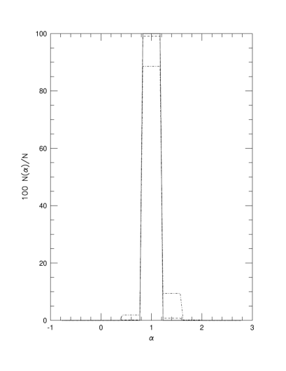
Fig. 2: The percentage ($100N(\alpha)/N)$ of the distribution of $\alpha$ in bins with the interval $\mathchar 28929\relax\alpha=0.4$, for $D_{\rm lA}$ in the lens model 2 and model S with $(1.0,0)$. The lines have the same meaning as in Fig. 1.

Fig. 3: The percentage ($100N(\alpha)/N)$ of the distribution of $\alpha$ in bins with the interval $\mathchar 28929\relax\alpha=0.4$, for $D_{\rm aA}$ in the lens model 1 and model S with $(1.0,0)$. The lines have the same meaning as in Fig. 1.

Fig. 4: The percentage ($100N(\alpha)/N)$ of the distribution of $\alpha$ in bins with the interval $\mathchar 28929\relax\alpha=0.4$, for $D_{\rm aA}$ in the lens model 2 and model S with (1.0, 0). The lines have the same meaning as in Fig. 1.

Fig. 5: The percentage ($100N(\alpha)/N)$ of the distribution of $\alpha$ in bins with the interval $\mathchar 28929\relax\alpha=0.4$, for $D_{\rm lA}$ in the lens model 1 and model L with $(0.2,0.8)$. The lines have the same meaning as in Fig. 1.

Fig. 6: The percentage ($100N(\alpha)/N)$ of the distribution of $\alpha$ in bins with the interval $\mathchar 28929\relax\alpha=0.4$, for $D_{\rm lA}$ in the lens model 2 and model O1 with (0.2, 0.8). The lines have the same meaning as in Fig. 1.

Table I: The average clumpiness parameter $\bar{\alpha}$ and its dispersion $\sigma_{\alpha}$, and the average normalized distance $\bar{d}_{\rm A}$ and its dispersion $\sigma_{d}$ for two lens models in model S with $(\mathchar 28938\relax_{0},\lambda_{0})=(1.0,0)$.  

			linear	$(D_{\rm lA})$			area	$(D_{\rm aA})$
lens	$z$	$\bar{\alpha}$	$\sigma_{\alpha}$	$\bar{d}_{\rm A}$	$\sigma_{d}$	$\bar{\alpha}$	$\sigma_{\alpha}$	$\bar{d}_{\rm A}$	$\sigma_{d}$
	0.5	$1.09$	$0.43$	1.00	0.018	$1.09$	$0.36$	1.00	0.015
	1	$1.03$	$0.25$	1.00	0.032	$1.04$	$0.22$	1.00	0.028
1	2	$1.02$	$0.15$	0.99	0.051	$1.03$	$0.41$	0.99	0.045
	3	$1.01$	$0.11$	0.99	0.063	$1.02$	$0.10$	0.99	0.056
	4	$1.01$	$0.09$	0.99	0.073	$1.02$	$0.08$	0.99	0.064
	5	$1.01$	$0.08$	0.99	0.080	$1.02$	$0.07$	0.99	0.071
	0.5	$1.09$	$0.28$	1.00	0.012	$1.07$	$0.23$	1.00	0.009
	1	$1.03$	$0.14$	1.00	0.019	$1.03$	$0.13$	1.00	0.017
2	2	$1.02$	$0.09$	0.99	0.029	$1.02$	$0.08$	0.99	0.027
	3	$1.01$	$0.07$	0.99	0.037	$1.02$	$0.06$	0.99	0.034
	4	$1.01$	$0.06$	0.99	0.043	$1.01$	$0.05$	0.99	0.040
	5	$1.01$	$0.05$	0.99	0.048	$1.01$	$0.04$	0.99	0.044

Table II: The average clumpiness parameter $\bar{\alpha}$ and its dispersion $\sigma_{\alpha}$, and the average normalized distance $\bar{d}_{\rm A}$ and its dispersion $\sigma_{d}$ for two lens models in model L with $(\mathchar 28938\relax_{0},\lambda_{0})=(0.2,0.8)$.  

			linear	$(D_{\rm lA})$			area	$(D_{\rm aA})$
lens	$z$	$\bar{\alpha}$	$\sigma_{\alpha}$	$\bar{d}_{\rm A}$	$\sigma_{d}$	$\bar{\alpha}$	$\sigma_{\alpha}$	$\bar{d}_{\rm A}$	$\sigma_{d}$
	0.5	$1.09$	$1.43$	1.00	0.019	$1.02$	$0.91$	1.00	0.012
	1	$1.07$	$1.15$	1.00	0.057	$1.02$	$0.69$	1.00	0.034
1	2	$1.02$	$0.68$	1.00	0.114	$1.03$	$0.49$	0.99	0.083
	3	$1.01$	$0.50$	1.00	0.157	$1.03$	$0.37$	0.99	0.118
	4	$1.00$	$0.39$	1.00	0.188	$1.02$	$0.29$	0.99	0.138
	5	$1.00$	$0.33$	1.00	0.211	$1.02$	$0.24$	0.99	0.155
	0.5	$1.08$	$0.43$	1.00	0.006	$1.06$	$0.29$	1.00	0.004
	1	$1.04$	$0.33$	1.00	0.016	$1.03$	$0.21$	1.00	0.010
2	2	$1.01$	$0.20$	1.00	0.034	$1.01$	$0.13$	1.00	0.022
	3	$1.01$	$0.15$	1.00	0.047	$1.01$	$0.10$	1.00	0.032
	4	$1.01$	$0.12$	1.00	0.056	$1.01$	$0.08$	1.00	0.039
	5	$1.01$	$0.10$	1.00	0.064	$1.01$	$0.07$	0.99	0.045

Fig. 7: The percentage ($100N(\alpha)/N)$ of the distribution of $\alpha$ in bins with the interval $\mathchar 28929\relax\alpha=0.4$, for $D_{\rm aA}$ in the lens model 1 and model O2 with $(0.2,0.8)$. The lines have the same meaning as in Fig. 1.

Fig. 8: The percentage ($100N(\alpha)/N)$ of the distribution of $\alpha$ in bins with the interval $\mathchar 28929\relax\alpha=0.4$, for $D_{\rm aA}$ in the lens model 2 and model O2 with (0.2, 0.8). The lines have the same meaning as in Fig. 1.

Fig. 9: The percentage ($100N(\alpha)/N)$ of the distribution of $\alpha$ in bins with the interval $\mathchar 28929\relax\alpha=0.4$, for $D_{\rm lA}$ in the lens model 1 and model O with $(0.2,0)$. The lines have the same meaning as in Fig. 1.

Fig. 10: The percentage ($100N(\alpha)/N)$ of the distribution of $\alpha$ in bins with the interval $\mathchar 28929\relax\alpha=0.4$, for $D_{\rm lA}$ in the lens model 2 and model O with (0.2, 0). The lines have the same meaning as in Fig. 1.

Fig. 11: The percentage ($100N(\alpha)/N)$ of the distribution of $\alpha$ in bins with the interval $\mathchar 28929\relax\alpha=0.4$, for $D_{\rm aA}$ in the lens model 1 and model O with $(0.2,0)$. The lines have the same meaning as in Fig. 1.

Fig. 12: The percentage ($100N(\alpha)/N)$ of the distribution of $\alpha$ in bins with the interval $\mathchar 28929\relax\alpha=0.4$, for $D_{\rm aA}$ in the lens model 2 and model L with (0.2, 0). The lines have the same meaning as in Fig. 1.

Table III: The average clumpiness parameter $\bar{\alpha}$ and its dispersion $\sigma_{\alpha}$, and the average normalized distance $\bar{d}_{\rm A}$ and its dispersion $\sigma_{d}$ for two lens models in model O with $(\mathchar 28938\relax_{0},\lambda_{0})=(0.2,0)$.  

			linear	$(D_{\rm lA})$			area	$(D_{\rm aA})$
lens	$z$	$\bar{\alpha}$	$\sigma_{\alpha}$	$\bar{d}_{\rm A}$	$\sigma_{d}$	$\bar{\alpha}$	$\sigma_{\alpha}$	$\bar{d}_{\rm A}$	$\sigma_{d}$
	0.5	$1.02$	$1.99$	1.00	0.020	$1.07$	$1.24$	1.00	0.012
	1	$1.07$	$1.55$	1.00	0.046	$1.12$	$1.22$	1.00	0.037
1	2	$1.06$	$1.06$	1.00	0.084	$1.09$	$0.84$	0.99	0.067
	3	$1.04$	$0.89$	1.00	0.113	$1.09$	$0.74$	0.99	0.094
	4	$1.03$	$0.82$	0.99	0.137	$1.08$	$0.68$	0.99	0.115
	5	$1.03$	$0.75$	0.99	0.156	$1.07$	$0.62$	0.99	0.129
	0.5	$1.08$	$0.61$	1.00	0.006	$1.04$	$0.44$	1.00	0.004
	1	$1.08$	$0.49$	1.00	0.014	$1.08$	$0.41$	1.00	0.012
2	2	$1.04$	$0.31$	1.00	0.025	$1.06$	$0.26$	1.00	0.021
	3	$1.03$	$0.26$	1.00	0.033	$1.06$	$0.22$	0.99	0.028
	4	$1.02$	$0.24$	1.00	0.040	$1.05$	$0.20$	0.99	0.034
	5	$1.02$	$0.22$	1.00	0.046	$1.05$	$0.18$	0.99	0.038

As a result of statistical analysis for this ray-shooting, we derived the average clumpiness parameter $\bar{\alpha}$, the average normalized distance $\bar{d}_{\rm A}$, their dispersions ($\sigma_{\alpha}$ and $\sigma_{d}$) and the distribution ($N(\alpha)$) of $\alpha$. Here, in order to study the frequency of ray pairs with $\alpha$, we consider many bins with the interval $\mathchar 28929\relax\alpha=0.4$ and the centers $\alpha_{i}=1.0\pm 0.4i\ (i=0,1,2,...)$. The number of ray pairs with $\alpha_{i}-\mathchar 28929\relax\alpha/2\leq\alpha\leq\alpha_{i}+\mathchar 28929\relax\alpha/2$ is expressed as $N(\alpha_{i})$ and the total number of ray pairs is $N(=\sum_{i}N(\alpha_{i}))$. In Tables I $\sim$ III, $(\bar{\alpha},\sigma_{\alpha},\bar{d_{\rm A}},\sigma_{d})$ for $D_{\rm lA}$ and $D_{\rm aA}$ in the two lens models are shown for models S, L and O, respectively. In Figs. 1 $\sim$ 12, the percentages of the distribution of $\alpha$, that is, $100N(\alpha)/N$ for $D_{\rm lA}$ and $D_{\rm aA}$ are shown for the above three models. The bar graphs in these figures have the same meaning as the line graphs which were used in the previous paper.[17] In Figs. 1, 5 and 9, the distributions for six values of $z$ are shown, and in the other figures those for only $z=1,3$ and $5$ are shown to avoid confusion. The following types of statistical behavior are found from these tables and figures :

(1) In all cases, both the average values $\bar{\alpha}$ and $\bar{d}_{\rm A}$ are nearly equal to $1$, so that the average angular distance can be regarded as the Friedmann distance.

(2) For each angular distance, the two kinds of dispersions have different behavior: $\sigma_{\alpha}$ increases in the order of O, L and S for the same value of $z$, and $\sigma_{\alpha}$ in a given universe model decreases with the increase of $z$. On the other hand, $\sigma_{d}$ increases in the order of L, O and S, and $\sigma_{\alpha}$ in a given universe model increases with the increase of $z$. This behavior is connected with the situation that the change in the Dyer-Roeder distance corresponding to the change in $\alpha$ is small for $\alpha<1$.

(3) Generally the dispersions for $D_{\rm lA}$ are larger than those for $D_{\rm aA}$, and the ratios of two dispersions are $\sim 1.2$ for model S and $\sim 1.6$ for models L and O. These differences can be seen also by comparing Figs. 1 and 3, Figs. 2 and 4, …, and Figs. 10 and 12.

(4) The dispersions in the lens model 2 are smaller than those in the lens model 1. The ratios of the former to the latter are $\sim 2/3,1/3,1/3$ for universe models S, L and O, respectively. These differences can be seen similarly by comparing Figs. 1 and 2, Figs. 3 and 4, …, and Figs. 11 and 12. In the two lens models of model S and in the lens model 2 of models L and O, the angular diameter distances can be regarded as the Friedmann distance, because of the small dispersions. In the lens model 1 of models L and O, however, we cannot always use the Friedmann distance, because of comparatively large dispersions.

Using numerical ray-shooting in the $N$-body-simulating clumpy cosmological models, we studied the statistical behavior of the angular diameter distances $D_{\rm lA}$ and $D_{\rm aA}$ and determined the clumpiness parameter $\alpha$ by comparing it with the Friedmann distance $(\alpha=1)$ and the Dyer-Roeder distance $(\alpha>0)$. Moreover, we studied the behavior of the normalized distance $d_{\rm A}$. The results show that all average values of $\alpha$ are nearly equal to 1, the dispersions of the linear distance are slightly larger than those of the area distance, and in the lens model 1 of models L and O, the dispersions are not so small, and we cannot use the Friedmann distance, while in the other cases we can use the Friedmann distance because of small dispersions.

In the above averaging process, all light rays were taken into account. If we consider only weakly deflected light rays as contributing to weak lensing, the dispersion $\sigma_{\alpha}$ will be slightly smaller than the values in the above tables. However, the contribution of strong lensing to $\sigma_{\alpha}$ is small because of its small frequency.

Finally, we touch on the estimate of lensing correction to source magnitudes based on Tables I $\sim$ III. Using $\sigma_{d}$ in the area distance it is given by

$$\mathchar 28929\relax m(z)={5\over 2}\log[1+2\sigma_{d}]=2.18\sigma_{d}$$ (4.10)

for the source at $z$. Its values for the lens model $(1,2)$ are

$\mathchar 28929\relax m(0.5)=(0.033,0.020),(0.026,0.009)$ and $(0.026,0.009),$

$\mathchar 28929\relax m(1.0)=(0.061,0.037),(0.074,0.022)$ and $(0.081,0.026)$

for models S, L and O, respectively. This $\mathchar 28929\relax m$ (for the separation angle $\theta=1$ arcsec) was derived independently of $\mathchar 28929\relax m$ (for the separation angle $\theta=2$ arcsec), shown in the §3 of Tomita, Premadi and Nakamura’s paper in this Supplement, but their values at $z=1$ are roughly consistent. The lensing correction to source magnitudes was also investigated by Holz in different lens models and inhomogeneous models.[43]

5 Shear effect on distances

As we have shown in §2, the evolution of a cross sectional area of a light ray bundle is determined by Ricci and Weyl focusing along the trajectory of the ray bundle. Ricci focusing is a convergency effect due to matter in the ray bundle. On the other hand, Weyl focusing is a result of the tidal shear on the ray bundle induced by the inhomogeneous distribution of matter.

One of the main difficulties in deriving a distance-redshift relation analytically for a realistic inhomogeneous universe lies in estimating the effect of Weyl focusing on ray bundles.

Since the pioneering work of Gunn, [44] there has been a great deal of progress in constructing an analytical approach to investigate statistical quantities of realistic distances (e.g., dispersion and skewness of probability distribution of image magnifications). Babul and Lee, [45] among others, examined lensing magnification effects on distances due to the large scale structures ($\geq 0.5h^{-1}$Mpc, where Hubble constant $H_{0}=100h$km/sec/Mpc). They found that the dispersion in image magnifications is negligible even for sources at a redshift of 4. At the same time, they pointed out that the dispersion is very sensitive to the nature of the matter distribution on small scales. In their study, the effects of Weyl focusing were neglected based, on a numerical study by Jaroszyński et al. [46] in which the lensing magnification effects due to large scale structure ($\geq 1h^{-1}$Mpc) in cold dark matter models were examined, and it was concluded that Weyl focusing has no significant effect on image magnifications. Frieman [47] improved Babul and Lee’s study to reflect the recent developments in numerical and observational studies of large scale structure. Although he took small scale nonlinear structure into account, Weyl focusing effects were neglected without any reasonable basis.

Nakamura [22] examined the effects of shear on image magnification in the cold dark matter model universe with a linear density perturbation. He found that the effect is sufficiently small and concluded that Weyl focusing can be safely neglected for a light ray passing through linear density inhomogeneities.

The above cited studies mainly focus on large scale inhomogeneities, whereas the effects of small scale objects, such as galaxies and clusters of galaxies, have not been satisfactorily taken into account. It is, however, not clear whether the Weyl focusing effect due to small scale inhomogeneities has a significant effect on distances. In this section, we discuss the Weyl focusing effect due to small scale inhomogeneities, mainly following Hamana. [48]

5.1 Basic equations

We first derive an evolution equation of lensing magnification from the null geodesic equation, [49] which is equivalent to the optical scalar equations,[25, 50] and is convenient to examine gravitational lensing effects.

We rewrite the cosmological Newtonian metric (1.2) as

$$ds^{2}=a^{2}(\eta)\left[-(1+2\mathchar 28936\relax)d\eta^{2}+(1-2\mathchar 28936\relax)\gamma_{ij}dx^{i}dx^{j}\right],$$ (5.1)

where $\eta$ is a conformal time: $d\eta\equiv cdt$. We write the above metric as $g_{\mu\nu}=a^{2}\hat{g}_{\mu\nu}$. Since the light cone structure is invariant under the conformal transformation of the metric, in the following we work in conformally related $\hat{g}$ world.

Let us consider an infinitesimal bundle of light rays intersecting at the observer. We denote a connecting vector which connects the fiducial light ray $\gamma$ to one of its neighbors as $\xi^{\mu}$. All gravitational focusing and shearing effects on the infinitesimal light ray bundle are described by the geodesic deviation equation,

$${{d^{2}\xi^{\mu}}\over{d\lambda^{2}}}=-{R^{\mu}}_{\alpha\nu\beta}\xi^{\nu}k^{\alpha}k^{\beta},$$ (5.2)

where $k^{\alpha}=dx^{\alpha}/d\lambda$, and $\lambda$ is the affine parameter along the fiducial light ray $\gamma$. We introduce a dyad basis $e_{\mu}{}^{A}$ ($A$, $B$, $C,...=1,2$) in the two-dimensional screen orthogonal to $k^{\mu}$ and parallel-propagated along $\gamma$. The screen components of the connection vector are given by

$$Y^{A}=e_{\mu}{}^{A}\xi^{\mu}.$$ (5.3)

From the geodesic deviation equation (5.2), one can immediately find that $Y^{A}$ satisfies the Jacobi differential equation

$${{d^{2}Y_{A}}\over{d\lambda^{2}}}={\cal{T}}_{AB}Y^{B},$$ (5.4)

where ${\cal{T}}_{AB}$ is the so-called optically tidal matrix. [50] From the metric (5.1), up to first order in $\mathchar 28936\relax$, this matrix is given by

$$\mbox{{\boldmath${\cal{T}}$}}=-K\mbox{{\boldmath${\cal{I}}$}}-\left(\begin{array}[]{ll}{\cal{R}}+\mbox{Re}\left[{\cal{F}}\right]&\mbox{Im}\left[{\cal{F}}\right]\\ \mbox{Im}\left[{\cal{F}}\right]&{\cal{R}}-\mbox{Re}\left[{\cal{F}}\right]\end{array}\right),$$ (5.5)

where ${\cal{I}}$ is the $2\times 2$ identity matrix, and ${\cal{R}}$ and ${\cal{F}}$ represent the Ricci and Weyl focusing induced by the density inhomogeneities, respectively:

$${\cal{R}} = \mathchar 28929\relax^{(3)}\mathchar 28936\relax={{3\mathchar 28938\relax_{0}H_{0}^{2}}\over{2}}{{\delta}\over a},$$ (5.6)

$${\cal{F}} = \mathchar 28936\relax_{,11}-\mathchar 28936\relax_{,22}+2i\mathchar 28936\relax_{,12}.$$ (5.7)

Here $\mathchar 28929\relax^{(3)}$ is the Laplacian operator in the spatial section, and $\delta$ is the density contrast defined by $\delta\equiv(\rho-\rho_{b})/\rho_{b}$, where $\rho_{b}$ is the mean matter density. Owing to the linearity of (5.4), the solution of $Y^{A}$ can be written in terms of its initial value $dY^{A}/d\lambda|_{\lambda=0}=\vartheta^{A}$ and the $\lambda$-dependent linear transformation matrix ${\cal{D}}_{AB}$ can be written as

$$Y^{A}(\lambda)={\cal{D}}^{A}{}_{B}(\lambda)\vartheta^{B}.$$ (5.8)

Substituting the last equation into the Jacobi differential equation (5.4), we obtain

$${{d^{2}{\cal{D}}_{AB}}\over{d\lambda^{2}}}={\cal{T}}_{AC}{\cal{D}}_{CB}.$$ (5.9)

Now, we derive an evolution equation of the lensing magnification matrix relative to the smooth Friedmann distance from (5.9). First, we write (5.5) as ${\cal{T}}$$=$${\cal{T}}$${}^{(0)}+$$\delta{\cal{T}}$, with ${\cal{T}}$${}^{(0)}=-K$${\cal{I}}$, and $\delta{\cal{T}}$ is the second term in (5.5). In the homogeneous case, $\delta{\cal{T}}$ is vanishing, and the solution of ${\cal{D}}$ is ${\cal{D}}_{AB}(\lambda)=D_{f}(\lambda)\delta_{AB}$, where $D_{f}$ is, of course, the standard angular diameter distance in the background Friedmann universe.

It is natural to define the lensing magnification matrix relative to the corresponding Friedmann universe as

$${\cal{M}}_{AB}(\lambda)\equiv{{{\cal{D}}_{AB}(\lambda)}\over{D_{f}(\lambda)}}.$$ (5.10)

Differentiating ${\cal{M}}_{AB}$ twice with respect to $\lambda$ and using (5.9), one finds

$${{d^{2}{\cal{M}}_{AB}}\over{d\lambda^{2}}}=-{2\over{D_{f}}}{{dD_{f}}\over{d\lambda}}{{d{\cal{M}}_{AB}}\over{d\lambda}}+\delta{\cal{T}}_{AC}{\cal{M}}_{CB}.$$ (5.11)

With the initial conditions ${\cal{M}}$$(\lambda)|_{\lambda=0}=$${\cal{I}}$ and $d$${\cal{M}}$ $(\lambda)/{d\lambda}|_{\lambda=0}=$${\cal{O}}$, [50] the last equation can be written in the integral form

$${\cal{M}}_{AB}(\lambda)=\delta_{AB}+\int_{0}^{\lambda}d\lambda^{\prime}{{D_{f}(\lambda-\lambda^{\prime})D_{f}(\lambda^{\prime})}\over{D_{f}(\lambda)}}\delta{\cal{T}}_{AC}(\lambda^{\prime}){\cal{M}}_{CB}(\lambda^{\prime}).$$ (5.12)

This is the general form of the evolution equation of the lensing magnification matrix relative to the Friedmann distance in multiple gravitational lensing theory. [2] Note, in general, this equation is not an explicit equation for ${\cal{M}}_{AB}$, since it involves an integration over the optical tidal matrix evaluated on the light ray path, such that one first has to solve a null geodesic equation. Since, for almost all cases of cosmological interest, the deflection angle is very small,[8] we will neglect the deflection of light rays.

5.2 Order-of-magnitude estimate

We now examine the magnitude of lensing effects on light ray bundles due to randomly distributed virialized objects (e.g. galaxies and clusters of galaxies) adopting an order-of-magnitude estimate. [8, 51] As can be seen in Eq. (5.12), if the magnitude of the components of the matrix, $\int d\lambda^{\prime}D_{f}(\lambda-\lambda^{\prime})D_{f}(\lambda^{\prime})/D_{f}(\lambda)\delta$$\cal{T}$$(\lambda^{\prime})$ is small, the magnitude of the lensing effects is dominated by these terms. We, therefore, examine the magnitude of these terms. For simplicity, we denote these terms as $\delta{\cal{M}}$.

Supposing that lensing objects are randomly distributed and that each has a mass $M=2{\sigma_{v}}^{2}l/G$, where ${\sigma_{v}}$ is the one-dimensional velocity dispersion of the lens objects, and $l$ is a characteristic comoving size of a lens object. Hence the mean comoving number density of the lens objects is

$$n_{L}={{3\mathchar 28938\relax_{L}{H_{0}}^{2}}\over{16\pi}}{1\over{\sigma_{v}}^{2}}{1\over{l}},$$ (5.13)

where $\mathchar 28938\relax_{L}$ is the density parameter of lens objects defined by $\mathchar 28938\relax_{L}\equiv\rho_{L}/(3H_{0}^{2}/8\pi G)$, with $\rho_{L}$ is the mean density of the lens objects. Thus, the mean comoving separation distance is

$$r_{0}=\left({{16\pi}\over{3\mathchar 28938\relax_{L}H_{0}^{2}}}\sigma_{v}^{2}l\right)^{1\over 3}.$$ (5.14)

Then for a geodesic affine comoving distance of $\lambda$, the light ray gravitationally encounters such objects $N_{g}=\lambda/r_{0}$ times on average. At each encounter, the contribution to the lensing magnification matrix is

$$\mathchar 28929\relax{\cal{M}} = 4\pi\left({{\sigma_{v}}\over c}\right)^{2}{{r_{0}}\over{b^{2}}}{{D_{f}(\lambda_{d})D_{f}(\lambda_{s}-\lambda_{d})}\over{D_{f}(\lambda_{s})}}$$ (5.15)

$$\sim 4\pi\left({{\sigma_{v}}\over c}\right)^{2}{1\over{r_{0}}}{{D_{f}(\lambda_{d})D_{f}(\lambda_{s}-\lambda_{d})}\over{D_{f}(\lambda_{s})}},$$

where $D_{f}(\lambda_{i}-\lambda_{j})$ is the comoving angular diameter distance, the subscripts $d$ and $s$ indicate the lens and source, respectively, and $b$ is the comoving impact parameter. In the above expression, we have assumed that the mean comoving impact parameter is of order $r_{0}$. Since the sign of each contribution will be random, the total contribution to the lensing magnification matrix is

$$\delta{\cal{M}} \sim \mathchar 28929\relax{\cal{M}}\sqrt{N_{g}}$$ (5.16)

$$\sim \sqrt{3\over 4}\sqrt{\mathchar 28938\relax_{L}}\left[4\pi\left({{\sigma_{v}}\over c}\right)^{2}{1\over{l}}{c\over{H_{0}}}\right]^{1\over 2}\left\langle{{{H_{0}}\over c}{{{D_{f}(\lambda_{d})D_{f}(\lambda_{s}-\lambda_{d})}}\over{D_{f}(\lambda_{s})}}}\right\rangle\left[{{H_{0}}\over c}\lambda\right]^{1\over 2}$$

$$\sim \sqrt{\mathchar 28938\relax_{L}}\sqrt{\nu}\left\langle{{{H_{0}}\over c}{{{D_{f}(\lambda_{d})D_{f}(\lambda_{s}-\lambda_{d})}}\over{D_{f}(\lambda_{s})}}}\right\rangle\left[{{H_{0}}\over c}\lambda\right]^{1\over 2},$$

where $\nu$ is a compactness parameter of a lens object defined by $\nu\equiv 4\pi(\sigma_{v}/c)^{2}l^{-1}\\ \times(c/H_{0})$. The contribution from direct encounters can be similarly estimated by noting that the average number of encounters is

$$N_{d}={{l^{2}\lambda}\over{r_{0}^{3}}}={{3\mathchar 28938\relax_{L}{H_{0}}^{2}}\over{16\pi}}{1\over{\sigma_{v}}^{2}}l\lambda,$$ (5.17)

with each encounter contributing

$$\mathchar 28929\relax{\cal{M}}_{d}=4\pi\left({{\sigma_{v}}\over c}\right)^{2}{1\over l}{{D_{f}(\lambda_{d})D_{f}(\lambda_{s}-\lambda_{s})}\over{D_{f}{\lambda_{s}}}},$$ (5.18)

with random sign. The result turns out to be the same as that of gravitational distant encounters, given by Eq. (5.16). The comoving affine distance $\lambda$ becomes $c/H_{0}$ at the source redshift $z_{s}\sim 3$, and the averaged value of the distance combination over the lens redshifts is of order

$$\left\langle{{H_{0}}\over c}{{D_{f}(\lambda_{d})D_{f}(\lambda_{s}-\lambda_{d})}\over{D_{f}(\lambda_{s})}}\right\rangle\sim{\cal{O}}(0.1).$$ (5.19)

Accordingly, we find that the magnitude of the total contribution of the lensing effects to the lensing magnification matrix scales as $\sim 0.1\sqrt{\mathchar 28938\relax_{L}}\sqrt{\nu}$ for the source redshift $z_{s}\sim 3$. We have the relation $\mathchar 28938\relax_{L}\leq\mathchar 28938\relax_{0}$ by definition, and $\mathchar 28938\relax_{0}$ appears to be less than unity. Thus $\mathchar 28938\relax_{L}\leq 1$. On the other hand, $\nu\leq 1$ for galaxies and clusters of galaxies. Therefore a typical value of gravitational lensing effects on the lensing matrix can be expected to be ${\cal{O}}(0.1)$ or smaller for a majority of random lines of sight.

The lensing magnification factor of a point like image is defined by the determinant of the lensing magnification matrix. Taking the determinant of the lensing magnification matrix (5.12), and expanding it in powers of $\delta{\cal{M}}$, one can easily find that the leading term of Weyl focusing effects is of order $\delta{\cal{M}}^{2}$. On the other hand, that of the Ricci focusing term is of order $\delta{\cal{M}}$. Since we have seen that a typical value of $\delta{\cal{M}}$ is expected to be ${\cal{O}}(0.1)$ or smaller, we can conclude that, at least from a statistical point of view, Weyl focusing has no significant effects on the image magnifications or equivalently on the distances.

5.3 Numerical investigation

The above argument may sound too naive. One of the authors (T.H.), numerically investigated Weyl focusing effects on image magnifications by using the multiple gravitational lens theory.[48] He focused on gravitational lensing effects due to small scale virialized objects, such as galaxies and clusters of galaxies. He considered a simple model of an inhomogeneous universe. The matter distribution in the universe was modeled by randomly distributed isothermal objects. He found that, for the majority of the random lines of sight, Weyl focusing has no significant effect, and the image magnification of a point like source within a redshift of 5 is dominated by Ricci focusing. He also found that his result agrees well with the order-of-magnitude estimate given above.

To summarize, we conclude that, except for a statistically very rare kind of light ray, Weyl focusing has no significant effect on image magnifications or equivalently on the distances.

6 Concluding remarks

Lensing observation in inhomogeneous universes was discussed in §3, based on the so-called Dyer-Roeder distance, in which one of the main assumptions is neglecting Weyl focusing. Such a neglection seems correct in our universe, as was shown in the §5.

The average angular distances in inhomogeneous model universes are the Friedmann distances, as was shown in §4, but individual ray bundles have various values of clumpiness parameters $\alpha$ because of their dispersions. The observational quantities are sensitively dependent on $\alpha$, as was shown in the §3, and so they may have dispersions similar to $\alpha$.

The difference between linear and area angular diameter distances, which is caused by the shear, is generally small in accord with the result in §5, even though we considered small-scale inhomogeneities, but the difference in the low-density models is found to be larger than that in the Einstein-de Sitter model. This implies that the shear effect is comparatively larger in the low-density models.

References

- [1] S. Weinberg, Gravitation and Cosmology (Wiley, New York, 1972).
- [2] P. Schneider, J. Ehlers and E. E. Falco, Gravitational Lenses (Springer-Verlag, New York, 1992), p. 157.
- [3] H. Nariai and Y. Ueno, Prog. Theor. Phys. 23 (1960), 305.
- [4] Y. M. Irvine, Ann. of Phys. 32 (1965), 322.
- [5] T. Futamase, Phys. Rev. Lett. 61 (1988), 2175.
- [6] K. Tomita, Prog. Theor. Phys. 79 (1988), 258, 85 (1991), 1041.
- [7] M. Shibata and H. Asada, Prog. Theor. Phys. 94 (1995), 11.
- [8] T. Futamase and M. Sasaki, Phys. Rev. D40 (1989), 2502.
- [9] Ya. B. Zel’dovich, Soviet Astron.-AJ 8 (1964), 13.
- [10] V. M. Dashevskii and V. I. Slysh, Soviet Astron.-AJ 9 (1966), 671.
- [11] C. C. Dyer and R. C. Roeder, Astrophys. J. 174 (1972), L115.
- [12] C. C. Dyer and R. C. Roeder, Astrophys. J. 181 (1973), L31.
- [13] M. Fukugita, T. Futamase, M. Kasai and E. L. Turner, Astrophys. J. 393 (1992), 3.
- [14] H. Asada, Astrophys. J. 501 (1998), 473.
- [15] M. Kasai, T. Futamase and F. Takahara, Phys. Lett. A147 (1990), 97.
- [16] K. Watanabe and K. Tomita, Astrophys. J. 355 (1990), 1.
- [17] K. Tomita, Prog. Theor. Phys. 100 (1998), 79.
- [18] R.K. Sachs, Proc. Roy. Soc. London A264 (1961), 309.
- [19] S. Weinberg, Astrophys. J. 208 (1976), L1
- [20] K. Watanabe, M. Sasaki and K. Tomita, Astrophys. J. 394 (1992), 38.
- [21] K. Watanabe and M. Sasaki, Publ. Astron. Soc. Jpn. 42 (1990), L33.
- [22] T.T. Nakamura, Publ. Astron. Soc. Jpn. 49 (1997), 151.
- [23] P. Jordan, J. Ehlers and R. K. Sachs, Akad. Wiss. Mainz ( 1961), 1.
- [24] I. M. H. Etherington, Philos. Mag. 15 (1933), 761.
- [25] M. Sasaki, Prog. Theor. Phys. 90 (1993), 753.
- [26] P. Schneider and A. Weiss, Astrophys. J. 327 (1988), 526.
- [27] P. Schneider and A. Weiss, Astrophys. J. 330 (1988), 1.
- [28] C. C. Dyer and R. C. Roeder, Astrophys. J. 189 (1974), 167.
- [29] S. Refsdal, Mon. Not. R. Astron. Soc. 128 (1964), 295.
- [30] S. Refsdal, Mon. Not. R. Astron. Soc. 128 (1964), 307.
- [31] S. Refsdal, Mon. Not. R. Astron. Soc. 132 (1966), 101.
- [32] W. H. Press and J. E. Gunn, Astrophys. J. 185 (1973), 397.
- [33] R. Blandford and R. Narayan, Ann. Rev. Astron. Astrophys. 30 (1986), 311.
- [34] M. Fukugita, T. Futamase and M. Kasai, Mon. Not. R. Astron. Soc. 264 (1990), 24.
- [35] C. Alcock and N. Anderson, Astrophys. J. 291 (1985), L29.
- [36] H. Asada, Astrophys. J. 485 (1997), 460.
- [37] R. Kantowski, Astrophys. J. 155 (1969), 69.
- [38] E. V. Linder, Astron. Astrophys. 206 (1988), 190.
- [39] M. Kasai, T. Futamase and F. Takahara, Phys. Lett. A147 (1990), 97.
- [40] M. Bartelmann and P. Schneider, Astron. Astrophys. 248 (1991), 349.
- [41] Y. Suto, Prog. Theor. Phys. 90 (1993), 1173
- [42] E. Bertschinger, Astro-ph/9506070.
- [43] D. E. Holz, Astrophys. J. 506 (1998), L1.
- [44] J. E. Gunn, Astrophys. J. 150 (1967), 737.
- [45] A. Babul and M. H. Lee, Mon. Not. R. Astron. Soc. 250 (1991), 407.
- [46] M. Jaroszyński, C. Park, B. Paczyński and J. R. Gott, Astrophys. J. 365 (1990), 22.
- [47] J. A. Frieman, Comments Astrophys. 18 (1997), 323.
- [48] T. Hamana, Mon. Not. R. Astron. Soc. 302 (1999), 801.
- [49] T. Hamana, Prog. Theor. Phys. 99 (1998), 1085.
- [50] S. Seitz, P. Schneider and J. Ehlers, Class. Quant. Gravi. 11 (1994), 2345.
- [51] P. J. E. Peebles, Principles of Physical Cosmology (Princeton: Princeton Univ. Press., 1993)