Detection Efficiencies of Microlensing Datasets to Stellar and Planetary Companions

Abstract

Microlensing light curves are now being monitored with the temporal sampling and photometric precision required to detect small perturbations due to planetary companions of the primary lens. Microlensing is complementary to other planetary search techniques, both in the mass and orbital separation of the planets to which it is sensitive and its potential for measuring the statistical frequency of planets beyond the solar neighborhood. We present an algorithm to analyze the efficiency with which the presence of lensing binaries of given mass ratio and angular separation can be detected in real microlensing datasets. Such an analysis is required in order to draw statistical inferences about lensing companions, and differs from previous studies of idealized microlensing experiments by incorporating instead the actual sampling, photometric precision, and monitored duration of individual light curves. We apply the method to artificial (but realistic) data to explore the dependence of detection efficiencies on observational parameters, the impact parameter of the event, the finite size of the background source, the amount of unlensed (blended) light, and the criterion used to define a detection. We find that: (1) the integrated efficiency depends strongly on the impact parameter distribution of the monitored events, (2) calculated detection efficiencies are robust to changes in detection criterion for strict criteria ($\Delta\chi^{2}{{}_{>}\atop{}^{{}^{\sim}}}100$) and large mass ratios $(q{{}_{>}\atop{}^{{}^{\sim}}}10^{-2}$), (3) finite sources can dramatically alter detection efficiencies to companions with mass ratios $q{{}_{<}\atop{}^{{}^{\sim}}}10^{-3}$, and (4) accurate determination of the blended light fraction is crucial for the accurate determination of the detection efficiency of individual events. Suggestions are given for addressing complications associated with computing accurate detection efficiencies of real datasets.

1. Introduction

The discovery in 1995 of a massive planet orbiting 51 Peg (Mayor & Queloz (1995)) followed by the discovery of several more planets orbiting nearby dwarf stars using the same radial velocity technique (see Marcy & Butler (1998) and references therein) has focussed both public and scientific attention on the search for extra-solar planets and the experimental and theoretical progress being made in developing other viable detection techniques.

Due to their small mass and size, extra-solar planets are difficult to find. Proposed detection methods can be subdivided into direct and indirect techniques. Direct methods rely on the detection of the reflected light of the parent star, and are exceedingly challenging due to the extremely small flux expected from the planet, which is overwhelmed by stray light from the star itself (Angel & Woolf (1997)). Some direct imaging searches have already been performed (Boden et al. 1998b ), but the future of this method lies in the construction and launching of a space-based interferometer (Woolf & Angel (1998)).

Astrometric, radial velocity and occultation measurements can be used to detect the presence of a planet indirectly. Astrometric detection relies on the measurement of the wobble of the stellar centroid caused by the motion of the star around the center-of-mass of the planet-star system, and yields the mass ratio of the planet-star system. Many attempts to find extra-solar planets in this way have been made, but the measurements are difficult and the detections remain controversial; planned space-based missions are expected to be more successful (Lindegren & Perryman (1996)). Occultation methods use very accurate photometry of the parent star to detect the small decrease in flux (${{}_{<}\atop{}^{{}^{\sim}}}1\%$) caused by a planet transiting the face of the star (Hale & Doyle (1994)). Occultation searches are currently being carried out (Deeg et al. (1998)), and spaced-based missions are planned to increase the sensitivity to small-mass planets (Deleuil et al. (1997), Borucki et al. (1997)). By far the most successful indirect method for discovering planets has been the Doppler technique, which employs extraordinarily precise radial velocity measurements of nearby stars to detect Doppler shifts caused by orbiting planets. Several teams have monitored nearby stars with the aim of detecting the Doppler signal of orbiting planets (McMillan et al. (1993); Mayor & Queloz (1995); Butler et al. (1996), Cochran et al. (1997), Noyes et al. (1997)). To date these groups combined have discovered over 20 extra-solar planets using this technique, with new planetary companions being announced every few months (Marcy & Butler (1998)). Of these techniques, only the proposed space-based interferometric imaging and transit searches are expected to be sensitive to Earth-mass planets.

These detection techniques are complementary to one another both in terms of their sensitivity to planetary mass and orbital separations and the specific physical quantities of the planetary system that they measure. All share two distinct advantages: the experiments are repeatable and, due to their reliance on flux measurements of the parent star or the planet itself, they are sensitive to stars in the solar neighborhood where follow-up studies can be most easily pursued. For example, spectroscopic follow-up studies may enable the detection of molecules commonly thought to be indicative of life, such as water, carbon dioxide, and ozone (Woolf & Angel (1998)). This advantage is linked to a common drawback: the searches can be conducted only on a limited number of nearby stars. Without substantial developments in technology beyond what is currently available, these methods are unlikely to detect planets orbiting stars more distant than $\sim$1$\,{\rm kpc}$, and are thus unable to address questions about the nature of planetary systems beyond the immediate solar neighborhood.

Microlensing was proposed in 1986 by Paczyński as a method to detect compact baryonic dark matter in the halo of our Galaxy. Soon after, three collaborations (MACHO, Alcock et al. (1993); EROS, Aubourg et al. (1993); OGLE, Udalski et al. (1993)) were organized to implement this proposal with massive observational programs. The basic idea is simple: when a compact object, such as a star or massive dark object, passes near the line of sight to a distant source, the gravitational field of the intervening object will serve as a lens, creating two images of the distant source. For typical stellar sources and lenses in our Galaxy, the separation of the images will be on the order of milliarcseconds and hence unresolved. However, the lens will also magnify the source; this magnification is measurable and depends (only) on the angular separation of the lens and source. Since the lens, source, and observer are all in relative motion, the magnification will be time-variable, creating a “microlensing event.” Because the probability that any single source star will be microlensed (the ‘optical depth’) is so low, ${\cal O}(10^{-6})$, millions of stars must be monitored; the crowded fields towards the Large and Small Magellenic clouds (LMC and SMC) and the Galactic bulge were thus the natural targets. In 1993, the first candidate microlensing events were announced toward the LMC (Alcock et al. (1993); Aubourg et al. (1993)) and Galactic bulge (Udalski et al. (1993)). Six years later, these three ‘survey teams’ continue to search and discover microlensing events. Over $400$ events have been discovered toward all three targets (MACHO, Alcock et al. 1997a, 1997b, 1997c; EROS, Renault et al. (1998), Palanque-Delabrouille et al. (1998); OGLE, Udalski et al. (1997)), the overwhelming majority of which are discovered toward the Galactic bulge.

Although Paczyński’s original suggestion was to search for dark matter, before the first event was discovered Mao & Paczyński (1991) had already noted that it might be possible to detect planetary companions of the primary microlenses via the distortions they create in the magnification pattern, and thus the light curve, generated by the primary lens. The nature of the distortion depends on the mass ratio and angular separation of the two components.

As a planet search technique, microlensing offers unique advantages. Since microlensing is caused the gravitational field (i.e., mass) of the lenses, it is not limited to the study of nearby or indeed luminous objects, and thus can be used to search for planetary companions around typical Galactic stars at distances of many kiloparsecs. As a consequence, a nearly unlimited number of dwarf stars are available to serve as gravitational microlenses and potential search candidates. This advantage is linked to the primary drawback of microlensing planetary searches: most follow-up studies will be difficult due to the faintness of the stars serving as typical lenses. This drawback is compounded by the irrepeatability of specific microlensing observations; lensing of a particular source by a particular lens is a singular occurrence. Nevertheless, the robust statistics on the nature of planetary systems many kiloparsecs distant and the complementary nature of the information about discovered systems microlensing can provide make it an important tool in the cadre being assembled to study extra-solar planets (Sackett 1999a ). Furthermore, microlensing planet searches are relatively inexpensive, requiring only several dedicated $1$-meter class telescopes. Microlensing is the only technique currently capable of routinely discovering planets like our own Jupiter, and the only ground-based method capable, in principle, of detecting distant terrestrial-mass planets, though this will require substantial enhancements over existing capabilities (Bennett & Rhie (1996); Peale (1997), Sackett (1997)).

Current microlensing survey teams have sampling rates that are too large ($\sim$day) and/or photometric accuracies that are too poor ($\sim 5\%$) to detect and characterize these perturbations, but the nearly 100 real-time electronic alerts of on-going bulge events that they provide annually have become the primary targets for newly-formed microlensing planet searches. These new ‘monitoring teams’ (PLANET, Albrow et al. 1997, 1998; GMAN, Alcock et al. 1997d ; MPS, Rhie et al. (1999)) have formed with the express purpose of executing the nearly continuous temporal coverage and high photometric precision on real-time microlensing alerts necessary to detect deviations from the generic light curve of the sort expected from planetary and other microlensing anomalies (see e.g. Albrow et al. (1998)). The PLANET collaboration in particular has now monitored nearly 100 microlensing events with varying degrees of photometric sampling and precision (often $\sim$hourly with $\sim$2% over the largest magnification regions); such existing datasets may already place interesting constraints on the frequency of stellar binaries and planetary systems.

Like all planet search techniques, microlensing is not $100\%$ efficient, due to both intrinsic and observational limitations. The efficiency with which a given dataset will reveal the presence of a companion to the primary microlens must be quantified before it can be used to constrain the frequency and properties of extra-solar planetary systems. Quantification of detection efficiencies of any kind can be a difficult and tedious process: the intrinsic limitations of the method must be identified and combined with the actual observational limitations. The detection efficiency may depend on hidden or unmeasurable parameters; these must be identified and properly quantified in order to avoid biasing the final conclusions. Detection efficiencies of other planet search techniques have been presented and applied to data (Nelson & Angel (1998)). However, despite a substantial body of work addressing the likely planet detection efficiency of idealized microlensing programs (see § 3), no methods have yet been proposed for calculating the efficiency of actual datasets to lensing binaries of a given type.

Here we present an algorithm for computing the detection efficiency to lensing binaries that is specific to individual microlensing light curves. By directly imposing the actual observational limitations as a constraint, the approach is less prone to the biases that may arise when using simplified models of observational conditions. Furthermore, the method is simple to implement and computationally inexpensive, since it involves direct integration over unknown quantities rather than Monte Carlo simulations commonly used to calculate detection efficiencies of idealized observing programs. We apply this method to simulated datasets in order to explore how the detection efficiency depends on intrinsic and observational effects. We also explore possible biases that may be introduced into the inferred efficiency of individual events to planet detection if the size of the source and the fraction of unresolved light (‘blending’) are ill-constrained.

In § 2, we review the relevant formalism for microlensing by single and double stars. A brief review of the literature on expectations for idealized microlensing planet searches is presented in § 3, contrasting these to the goal of this paper. Detection and detection efficiency, as used throughout this work, are defined in § 4, along with a general overview of the connection between detection efficiency and the mass ratio, angular separation and impact parameter of the event. Our algorithm for computing detection efficiencies is described in § 5 and applied to artificial data in order to access the effects of different detection criterion. The effects of finite source size on detection efficiencies are presented in § 6; the effects of blending in § 7. Suggestions for addressing complications associated with computing accurate detection efficiencies of real microlensing datasets are given in § 8. We summarize and conclude in § 9.

Figure 1.— Top panel: Magnification as a function of time in days for a microlensing event with (solid curve) and without (dotted curve) the presence of a companion with mass ratio $q=10^{-2}$. The event has an Einstein time scale of $t_{E}=30~{}{\rm{days}}$ and minimum impact parameter in units of the Einstein ring radius of ${u_{\rm min}}=0.5$. The single lens curve reaches a maximum magnification of $A_{\rm max}=2.2$ at a time $t_{0}=15~{}{\rm{days}}$. The binary lens curve was generated assuming that the source trajectory makes angle $\theta=300^{\circ}$ with respect to the binary axis. Also shown is the best single-lens fit to the binary-lens light curve (dashed curve). Bottom panel: The fractional deviation $\delta$ of the binary-lens light curve from the single-lens light curve with parameters $t_{E}=30~{}{\rm{days}},{u_{\rm min}}=0.5,t_{0}=15~{}{\rm days}$ (solid curve) and from the best fit single-lens light curve (dashed curve).

2. Relevant Formalism for Single and Double Microlenses

2.1. Single lenses

The time-variable flux observed from a microlensed star is

$$F(t)=F_{0}[A(t)+f_{B}]~{}~{}~{},$$ (1)

where $F_{0}$ is the unlensed flux of the star, $f_{B}$ is the ratio of any unresolved, unlensed background light to $F_{0}$ (the ‘blend fraction’), and $A(t)$ is the magnification. The magnification of $A_{0}$ of a point source by a point lens can be written as

$$A_{0}={{u^{2}+2}\over u(u^{2}+4)^{1/2}}~{}~{}.$$ (2)

Here $u$ is the instantaneous angular separation of the source and the lens in units of the angular Einstein ring radius $\theta_{E}$ of the lens, a degenerate combination of the lens mass and and distances defined by

$$\theta_{E}\equiv\left[{4GM\over c^{2}}{D_{LS}\over D_{OL}\,D_{OS}}\right]^{1/2}\sim 130\,\mu{\rm as}\left({M\over 0.2M_{\odot}}\right)^{1/2},$$ (3)

where $M$ is the mass of the lens, and ${D_{\rm LS}}$, ${D_{\rm OS}}$, ${D_{\rm OL}}$ are the lens-source, observer-source, and observer-lens distances, respectively. For the scaling relation on the far right of equation (3), we have assumed ${D_{\rm OL}}=6~{}{\rm kpc}$ and ${D_{\rm OS}}=8~{}{\rm kpc}$. Note that for $u\rightarrow 0$, $A_{0}\rightarrow 1/u$. Since the source, lens, and observer are all in relative motion, $u$ will be a function of time. For rectilinear motion, it can be shown that

$$u(t)=\left[\left({t-t_{0}\over t_{E}}\right)^{2}+u^{2}_{\rm min}\right]^{1/2},$$ (4)

where $t_{0}$ is the time of maximum magnification, ${u_{\rm min}}$ is the minimum angular separation, or impact parameter, of the event in units of $\theta_{E}$, and $t_{E}$ is a characteristic time scale of the event, the Einstein time, defined by

$$t_{E}={\theta_{E}{D_{\rm OL}}\over v_{\perp}}\sim 10~{}{\rm days}\left({M\over 0.2M_{\odot}}\right)^{1/2}.$$ (5)

Here $v_{\perp}$ is the transverse velocity of the lens relative to the observer-source line-of-sight. For the scaling relation on the far right of equation (5), we have assumed ${D_{\rm OL}}=6~{}{\rm kpc}$, ${D_{\rm OS}}=8~{}{\rm kpc}$, and $v_{\perp}=100~{}{\rm km\,s^{-1}}$.

A point-lens point-source (PSPL) light curve is thus a function of five parameters, $t_{0}$, $t_{E}$, ${u_{\rm min}}$, $F_{0}$, and $f_{B}$. Unless the lens is measurably luminous, the parameters $F_{0}$ and $f_{B}$ depend only on the source and its environment. The distributions of $F_{0}$ and $f_{B}$ depend on the luminosity functions of the observed sources and any blended light. The parameters $t_{0}$ and ${u_{\rm min}}$ are purely geometrical. Since the distribution of $t_{0}$ is flat and its value has no effect on the analysis of detection efficiencies, we will hereafter set $t_{0}=0$. The intrinsic distribution of ${u_{\rm min}}$ is also flat, but the observed distribution has an upper limit set by the detection threshold of the survey teams. If the lens is not contributing significantly to the blended light, only the characteristic time $t_{E}$ contains physical information about the lens itself. Its intrinsic distribution is set by the lens masses and spatial distribution of the lenses and sources; the observed distribution of $t_{E}$ depends on the temporal sampling of the microlensing campaigns. An example of a point-lens light curve with $t_{0}=15~{}{\rm days}$, $t_{E}=30~{}{\rm days}$, ${u_{\rm min}}=0.5$, $F_{0}=1$, and $f_{B}=0$ is shown as the dotted line in the top panel of Figure 1.

2.2. Binary lenses

A companion orbiting a lens constitutes a double lens and thus can be described by the formalism of binary lenses. The flux is still expressed by equation (1), but the magnification can no longer be calculated analytically. Instead, the lens equation describing the mapping from the source plane ($\xi,\eta$) to the image plane ($x,y$) must be solved. Following Witt (1990), we write the lens equation for two masses with fractional mass $m_{1}$ and $m_{2}$ located at positions $z_{1}$ and $z_{2}$ in terms of the complex coordinates $\zeta\equiv\eta+i\xi$ and $z\equiv x+iy$,

$$\zeta=z+{m_{1}\over\bar{z}_{1}-\bar{z}}+{m_{2}\over\bar{z}_{2}-\bar{z}}~{}~{}.$$ (6)

Here all distances are in units of $\theta_{E}$, the Einstein ring radius of the total mass $M$ of the binary. The mapping is described completely by two parameters, the instantaneous angular separation of the two components in units of $\theta_{E}$, $b=|z_{1}-z_{2}|$, and the mass ratio of the system, $q=m_{2}/m_{1}$. Without loss of generality, we will assume that $m_{2}\leq m_{1}$, so that $q\leq 1$. Equation (6) is equivalent to a fifth-order complex polynomial in $z$, which can be solved by the usual techniques. Each source position produces either three or five images. The magnification $A_{j}$ of each image $j$ is inversely proportional to the determinant of the Jacobian of the lens mapping, evaluated at that image position,

$$A_{j}=\left.{1\over{|{\rm{det}}J|}}\right|_{z=z_{j}},\,\,\,{\rm{det}}J=1-{{\partial\zeta}\over{\partial{\bar{z}}}}\overline{{{\partial\zeta}\over{\partial{\bar{z}}}}}.$$ (7)

The total magnification is given by the sum of the individual magnifications, $A=\sum_{j}A_{j}$. The set of source positions for which the magnification is formally infinite, given by the condition ${\rm{det}}J=0$, defines a set of closed curves called caustics. Depending on the values of $b$ and $q$, a binary lens may have one, two, or three caustics; the multiplicity of images changes by two as the source crosses a caustic.

A static, point-source binary-lens light curve is a function of eight parameters. Two are identical to the point-lens case, $F_{0}$ and $f_{B}$. The equation for $t_{E}$ retains the same form, but the choice of the fiducial mass $M$ is arbitrary and can refer to the total mass of the binary or the mass of one of the components. For binaries, ${u_{\rm min}}$ refers to the minimum angular separation (in units of $\theta_{E}$) between the source and the origin of the binary system. The choice of origin is also arbitrary; popular choices are the position of center of mass, the position of one of the masses, or the midpoint between the two. Equation (4) still holds for static binaries, so that $t_{0}$ is the time at which $u={u_{\rm min}}$, but for binary lenses this need not be the time of maximum magnification. The mapping parameters $b$ and $q$, and the angle $\theta$ on the sky between source trajectory and the binary axis, are the final three binary lens parameters. In the case of a single lens, the lensing geometry is azimuthally symmetric, and $\theta$ is completely degenerate for any measured light curve.

The value of ${u_{\rm min}}$ has a large effect on the detection efficiency of a given light curve to lens binarity; smaller ${u_{\rm min}}$ events generally have higher efficiency. The Einstein time scale $t_{E}$ affects the detection efficiencies in that shorter time scale events will, in general, be less densely sampled by monitoring teams than longer time scale events. Blending complicates matters due to the ambiguity between light curves with different combinations of ${u_{\rm min}}$ and blend fraction $f_{B}$ (Woźniak & Pacyński 1997), which can lead to ill-determined detection efficiencies if the blend fraction is poorly constrained (§ 7).

The magnification patterns of close binaries ($b\ll 1$), wide binaries ($b\gg 1$), and binaries with small mass ratios ($q\ll 1$), can be written as mathematical perturbations to the single lens pattern (Dominik (1999)); the light curves they produce can be mistaken for those due to a single lens for a majority of source trajectories. The fractional deviation $\delta$, which is defined by

$$\delta(t)\equiv{A(t)-A_{0}(t)\over A(t)}~{},$$ (8)

where $A(t)$ is the binary-lens magnification and $A_{0}(t)$ is the magnification of the best-fit single-lens model, quantifies the degree to which a binary-lens light curve deviates from a best-fit single lens model as a function of time.

The best-fit single lens model need not have the same parameters $t_{0}$, $t_{E}$ and ${u_{\rm min}}$ as the underlying binary and will vary depending on the size and duration of the deviation, which is determined by the source trajectory $\theta$ and the binary-lens parameters $(b,q)$. The top panel of Figure 1 shows a light curve for binary system with $q=0.01$ and $b=1.0$, and two single-lens light curves: one assuming that the parameters $t_{E},t_{0},{u_{\rm min}}$ are the same as in the underlying system, and the other the best-fit single lens curve. In this particular instance, the difference between the two single-lens curves is not large, although this is not universally true (see § 5.1). The bottom panel shows the fractional deviation of the binary light curve from both single-lens light curves. In this example, the deviation is appreciable ($\delta>1\%$) for a large fraction of the light curve, but is large ($\delta>5\%$) for only $\sim 5~{}{\rm days}$, underscoring the need for high photometric precision in microlensing planet searches.

3. Detection Probabilities for Idealized Microlensing Planet Searches

The success of microlensing survey and monitoring teams in implementing massive observational programs has prompted, and in part been driven by, theoretical work outlining optimal observational strategies, expected detection probabilities for binary lens perturbations, and methods for characterizing and extracting additional information about the companions.

Using heuristic arguments based on rough scaling relations for the size of planetary caustics, Mao & Paczyński (1991) estimated in their seminal paper that 3% of microlensing light curves should cross caustics and thus show planetary deviations if all lens have a Jupiter-mass planet at instantaneous angular separations comparable to the Einstein ring radius of the primary. Randomizing the orbital phase and inclination of the orbital plane to obtain the distribution of angular separations $b\,\theta_{E}$ on the sky corresponding to a real orbital radius $a$, Gould & Loeb (1992) estimated that planets with characteristics like our own Jupiter and Saturn orbiting solar-type stars halfway to the Galactic center would have detection probabilities of 17% and 3%, respectively. Their substantial probability is based on the assumption non-caustic crossing perturbations as small as $\delta{{}_{>}\atop{}^{{}^{\sim}}}5\%$ can be detected regardless of their duration. Performing a similar study, Bolatto & Falco (1993) obtained a higher detection probability of $\sim$40% for Jovian-like planets, requiring that the integrated difference between the binary light curve and a single-lens light curve of the same impact parameter ${u_{\rm min}}$ exceed a threshold corresponding to a 10% deviation over 36 hours. Bennett & Rhie (1996) included for the first time the finite size of the source, enabling them to study planetary systems with mass ratios as low as $10^{-5}$, comparable to the mass ratio of the Earth and a parent star with mass $0.5M_{\odot}$, whose caustics are smaller than the angular size of typical source stars. They found a small but non-negligible detection probability of ${{}_{<}\atop{}^{{}^{\sim}}}2\%$ for such low-mass planets, assuming a 50% weather duty cycle for observations capable of detecting deviations as small as 4% and as brief as $t_{E}/200$ ($\sim$2.4 hour).

All of these studies have concentrated on companions with instantaneous angular separations in the “Lensing Zone,” a region defined by $0.6\leq b\leq 1.6$ in which planetary caustics may cross the source trajectory for events with ${u_{\rm min}}<1$, corresponding to an initial alerting magnification by the survey teams of $A>1.34$. Recently, Di Stefano & Scalzo (1999a, 1999b) have presented exhaustive studies of the probability of detecting planets in wide orbits that place gas giants like those in our own Solar System outside the Lensing Zone of typical lenses. They conclude that such events may be detectable as isolated short duration events, which will alter the time scale distribution of all microlensing events, or as repeating events as the source trajectory passes first near the primary and then near the companion on the sky. The observing and analysis strategies of the survey and monitoring programs must be altered to optimally detect such planetary deviations, which, by definition, occur when the source is outside the Einstein ring of the primary.

Wambsganss (1997) has demonstrated the extraordinary variety of perturbations that can be produced by given planetary systems depending on the trajectory of the source star. In principle, this variety might lead to ambiguity in the inferred properties of a lensing planet based on a measured light curve, a potentially serious difficulty for the characterization of detected planetary systems. Gaudi & Gould (1997) found that potentially severe fitting ambiguities of a factor of $\sim$20 in the measured mass ratio could plague light curves with planetary anomalies, but that these could be alleviated by dense and accurate sampling of the planetary perturbations or simultaneous optical/infrared photometry. Gaudi (1998) notes that planetary microlensing anomalies may also be mistaken for particular types of binary source events; the ambiguity can be mitigated with similar additional observations. Griest & Safizadeh (1998) showed that the planetary detection probabilities for high magnification events can be quite large since the source necessarily passes close to the central caustic generated by any binary. Using several detection criteria, they found that Jupiter-mass planets can be detected with $\sim$100% efficiency in events with ${u_{\rm min}}{{}_{<}\atop{}^{{}^{\sim}}}0.1$ ($A_{\rm max}{{}_{>}\atop{}^{{}^{\sim}}}10$) over a substantial range of parent-planet separations. Gaudi, Naber, & Sackett (1998) pointed out that this necessarily implies that the presence of multiple planets would be revealed in high magnification events, since all companions contribute to the central caustic. They also noted that unless the caustic morphology of higher multiplicity lensing systems is understood, fitting degeneracies will prevent the association of deviant light curves with well-characterized planets in such events.

Such considerations have led to detailed proposals for observational strategies designed to maximize the detection of planets via microlensing. For planets of all mass ratios, Peale (1997) has stressed the importance of a longitudinally-distributed network of southern telescopes for continuous monitoring, as has implemented by the PLANET collaboration since 1995 in its Jovian-mass search (Albrow et al. (1997), 1998). Sackett (1997) points out that the high burden of proof demanded of non-repeating microlensing events necessitates a high-sampling rate for proper characterization of planetary anomalies; this suggests a wide-field imager at an excellent site as an ideal component in any microlensing search effort aimed at small mass planets. Both studies conclude that tens of planets per year may be detected by aggressive programs if every microlens has a planet in its Lensing Zone.

4. Defining Detection Criteria and Efficiencies for Actual Datasets

Previous studies of detection probabilities of idealized microlensing planet searches (§ 3) differ in spirit and approach from the situation confronted by a researcher wishing to use an actual database of microlensing light curves to draw inferences about possible lensing companions. First, real light curves are irregularly sampled, each with its own and usually varying photometric precision. Second, only the post-alert portion of the light curve is available to current monitoring teams, resulting in differences in the monitored phase of each event. Third, the intrinsic impact parameter distribution of the events is altered by choices made by both the discovery and monitoring teams; the actual distribution cannot be assumed to be uniform over any interval. Finally, because the true lensing parameters are unknown, a binary lens fit must be compared to the best-fit single lens model for a given light curve, not to a single-lens model in which the companion has been removed (see Fig. 1). Previous studies that did not use the best-fit single-lens model as the null hypothesis when calculating detection probabilities for idealized searches have overestimated the true detection probability (§ 5.1). These differences motivate the detection criteria and method of calculating detection efficiencies for actual datasets that we now describe.

All light curves contain information about the presence of companions around Galactic lenses: obviously anomalous light curves signal the possible presence of a companion while light curves without a detectable anomaly signal the possible absence of (certain types of) companions. With real datasets, both statements are probabilistic: the presence or absence a particular type of lensing companion in a particular system can only be made with a certain degree of confidence. Ultimately, we seek a method to characterize this probability consistently for all light curves, whether obviously anomalous or not, so that the complete dataset can be used to constrain the distribution of planets and other companions in orbit around Galactic lenses.

Because most microlensing light curves do not show obvious anomalies indicative of companions, we begin here by quantifying the extent to which an apparently non-anomalous light curve can be taken as a sign that planetary companions of a given mass ratio $q$ and projected separation $b$ are truly absent in the microlensing system under consideration. The absence of an observed planetary anomaly may be due to insufficient sampling, photometric precision, or monitoring duration, rather than the absence of a planet. This means that the efficiency of detection must be computed separately for each event. Intrinsic parameters, such as source trajectory, source size, and blending, may also serve to ‘hide’ the planetary anomaly from the observer, and must be disentangled from observational effects both to compute detection efficiencies of individual datasets and to formulate future observing strategies which will maximize the detection probability.

Before we can begin to quantify the detection efficiency, $\epsilon_{i}(b,q)$, of a lensing binary with microlensing parameters $b,q$ using light curve $\ell_{i}$, we must define the meaning of ‘detection.’ Here, we will consider a planetary companion to a lens to be ‘detected’ in light curve $\ell_{i}$ if some combination of the intrinsic binary parameters $b,q$ and $\theta$ produces a substantially better fit (characterized by $\Delta\chi^{2}$) to the observed light curve than the best-fit single lens model. In making the comparison, the parameters $t_{0},t_{E},F_{0},{u_{\rm min}}$ and $f_{B}$ are allowed to vary to achieve the best fit in both the binary and single lens models. The meaning of ‘substantially better fit’ can be adjusted by altering the threshold value of $\Delta\chi^{2}_{\rm thresh}$ that $\Delta\chi^{2}=\chi^{2}_{\rm best\,single}-\chi^{2}_{\rm best\,binary}$ must exceed.

Since here we consider only light curves that are not obviously discrepant from PSPL (by the criterion above), the angle $\theta$ between the source trajectory and binary axis is degenerate, and can be assumed to be drawn from a random distribution over the full range $0<\theta\leq 2\pi$. By detection efficiency, $\epsilon_{i}(b,q)$, we will mean the probability that an actual planetary companion with mass ratio $q$ and instantaneous angular separation $b$ would be ‘detected’ by the criterion above in a given observed light curve $\ell_{i}$, assuming a random source trajectory. Only a subset of source trajectory angles will produce detections by this criterion. The efficiency incorporates both the intrinsic sensitivity of the observations to a given anomaly and the probability that such an anomaly occurs for random source trajectories. An efficiency $\epsilon_{i}(b,q)$ of zero implies that a lensing companion with characteristics $b$ and $q$ would always escape detection with these observations; $\epsilon_{i}(b,q)=1$ implies that the companions would always be detected (if present) with data of this type and quality regardless of source trajectory through the magnification pattern. This efficiency can then be used to place a confidence level on the non-detection of $b,q$ binary anomalies in a given light curve.

Note that in order to draw inferences about the non-detection of planetary companions of absolute mass $m_{p}$ (in $M_{\odot}$) and orbital radius $a$ (in AU), additional assumptions or information must be brought to bear on the distribution of lens masses and distances. Integrations over orbital phase and inclination then must be performed to deproject the instantaneous angular separation $b$ into a probabilistic distribution function for orbital radius $a$.

4.1. Qualitative effect of the Intrinsic Binary Parameters

In addition to its dependence on observational parameters, the detection efficiency of a given light curve will be a strong function of the intrinsic mass ratio $q$ and instantaneous binary separation $b$ of the lens system.

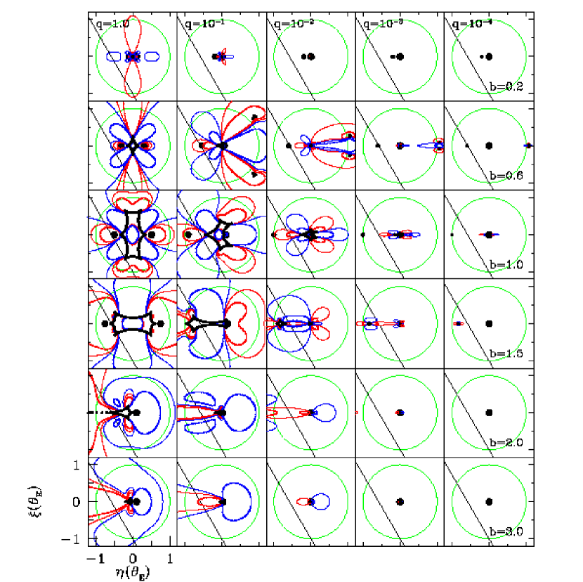
Figure 2.— Contours of fractional deviation $\delta$, for binary separations $b=0.2,0.6,1.0,1.5,2.0$, $3.0$ and mass ratios $q=1.0,10^{-1},10^{-2},10^{-3}$, $10^{-4}$, as a function of position in the source plane ($\eta,\xi$) in units of the Einstein ring radius of the binary, $\theta_{E}$. The red contours are $\delta=+0.01,+0.05$ (thin and heavy lines), the blue contours are $\delta=-0.01,-0.05$ (thin and heavy lines), and the heavy black lines are the caustics, $\delta=\infty$. The green circle is the Einstein ring. Black dots mark the positions of the lensing masses. The thin straight line is a trajectory with $u_{min}=0.5$ and $\theta=300$. Light curves for these trajectories are shown in Figure 3.

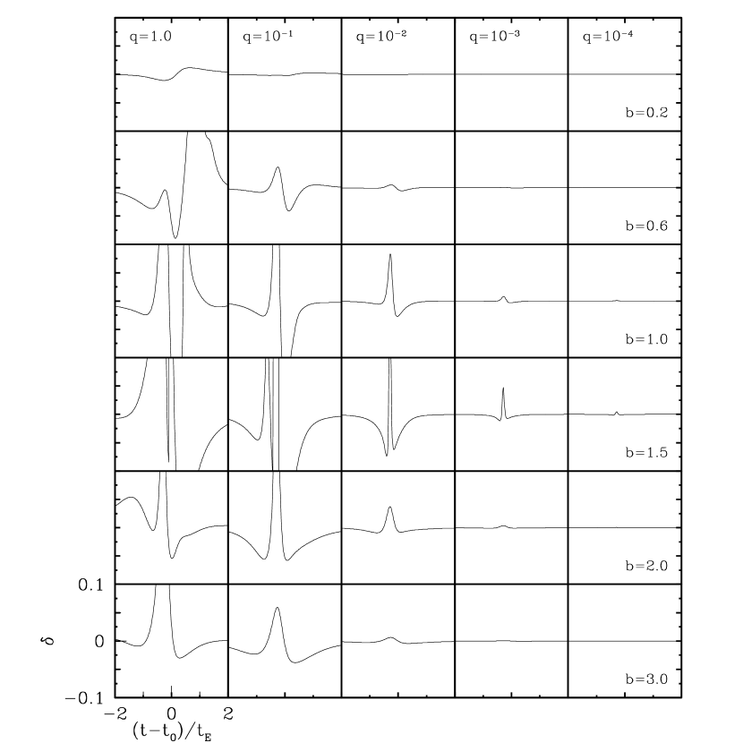
Figure 3.— The fractional deviation, $\delta$, from the single-lens light curve as function of time from the peak of the single lens light curve, $t_{0}$, in units of the Einstein ring crossing time $t_{E}$, for the trajectories shown in Figure 2.

Three limits are of special interest. First, as $b\rightarrow 0$, a binary lens reduces to a single lens, so that most light curves will have small detection efficiencies to binaries with small separations. Second, for $b\rightarrow 1$, a binary lens reduces to two isolated point lenses. Only small ${u_{\rm min}}$ trajectories with $\theta\sim 0$ (i.e. parallel to the binary axis) will betray the presence of both lenses (Di Stefano & Mao (1996)); most trajectories will produce light curves that are indistinguishable from single lens light curves. Finally, for $q\rightarrow 0$, a binary lens reduces to a single lens. Detection efficiencies thus will be highest for $q\sim 1$ and $b\sim 1$, and will decline for decreasing $q$ and outside an annulus centered near $b\sim 1$.

To illustrate these points, we calculate $\delta$ as a function source position $(\xi,\eta)$ for a grid of $b$ and $q$ values. Since the best-fit single lens light curve, and therefore $\delta$, depends on the exact trajectory, we must adopt heuristic approximations in order to display these qualitative results in a single plot of $\delta$ contours. For $b\leq 1.0$ and all $q$, we choose ${u_{\rm min}}$ to be the minimum projected separation from the center-of-mass, and normalize $t_{E}$ to the total mass of the binary. For $b>1.0$ and $q\leq 10^{-1}$, we choose ${u_{\rm min}}$ to be the minimum separation from the more massive lens component, and normalize $t_{E}$ to this component as well. For $q=1$ and $b=1.5$ we choose ${u_{\rm min}}$ to be the minimum projected separation from the center-of-mass, and normalize $t_{E}$ to the total mass of the binary. Finally, for $q=1$ and $b\geq 2.0$, we choose ${u_{\rm min}}$ to be the minimum separation from one of the components, and normalize $t_{E}$ to the same component. These choices were made in order to approximate the transition between close and wide binaries and minimize the deviation globally. Since this qualitative example does not use best-fit single lens parameters, $\delta$ will be overestimated in all cases; we discuss this effect fully in § 5.1. To cover the full range of parameter space for which the detection efficiency is high, we choose 5 values of $q$, logarithmically spaced between $1.0$ and $10^{-4}$, and $b=0.2$, $0.6$, $1.0$, $1.5$, $2.0$, and $3.0$. The results are shown in Figure 2, where contours of $\delta=\pm 0.01$ and $\pm 0.05$ are plotted with the caustics ($\delta=\infty$). Light curves are one-dimensional cuts through these diagrams. Since current survey programs rarely alert on-going events with ${u_{\rm min}}{{}_{>}\atop{}^{{}^{\sim}}}1$, only trajectories that pass within $\theta_{E}$ (circles in Figure 2) of the primary lens will be observed by the monitoring teams.

In Figure 3, light curves resulting from the sample trajectory in Figure 2 are displayed. This trajectory is rather typical, with ${u_{\rm min}}=0.5$ and a randomly chosen angle $\theta$. While for $q=1.0$ and $10^{-1}$, most trajectories will exhibit considerable ($\delta\geq 0.05$) deviations, for $q{{}_{<}\atop{}^{{}^{\sim}}}10^{-2}$, the magnitude of the deviation will depend strongly on the value of the $\theta$. For example, although the light curve in Figure 3 for $q=10^{-3}$ and $b=0.6$ exhibits no significant deviation, inspection of Figure 2 reveals that a trajectory with the same impact parameter but $\theta\sim 90^{\circ}$ would be likely to have larger $\delta$. This illustrates why a calculation of the detection efficiency of a non-anomalous light curve must involve an integration over $\theta$, which is degenerate in the single-lens case. Figures 2 and 3 also illustrate why the detection efficiency of a light curve depends strongly on its ${u_{\rm min}}$. The sample trajectory for $q=10^{-3}$ and $b=1.0$, for example, does not deviate more than $\delta\sim 0.05$, yet almost all trajectories with smaller ${u_{\rm min}}$ would exhibit much larger deviations.

Several conclusions can be drawn from inspection of Figures 2 and 3. First, for $q\sim 1$ and $0.2{{}_{<}\atop{}^{{}^{\sim}}}b{{}_{<}\atop{}^{{}^{\sim}}}3.0$, nearly all trajectories have deviations $\delta>5\%$. Second, for all separations $b$, events with ${u_{\rm min}}{{}_{<}\atop{}^{{}^{\sim}}}0.1$ will have a much higher detection efficiency than larger ${u_{\rm min}}$ events. Third, for small mass ratios ($q{{}_{<}\atop{}^{{}^{\sim}}}10^{-2}$), it is likely that only a small fraction of detected events will exhibit caustic crossings, since, for these mass ratios, the area covered by the caustics is considerably smaller than the area covered by the $\delta=\pm 0.05$ contours. Finally, for small $q$, detection efficiencies for light curves with typical impact parameters will be substantial only for companions with separations $0.6{{}_{<}\atop{}^{{}^{\sim}}}b{{}_{<}\atop{}^{{}^{\sim}}}1.6$ (i.e., in the ‘Lensing Zone’).

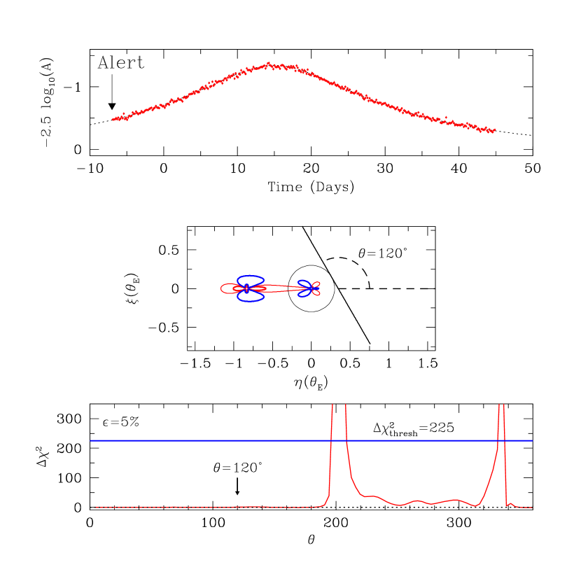
Figure 4.— Top panel: The difference in magnitude, $-2.5~{}\log_{10}(A)$, as a function of time for a simulated microlensing event with photometric precision of $2\%$ and with uniform sampling at the rate $t_{E}/200$ from alert until $t_{E}$. The dotted line shows the best-fit point-source point-lens (PSPL) event, which has parameters $t_{E}=15~{}{\rm days},{u_{\rm min}}=0.5,t_{0}=15~{}{\rm days}$. Middle panel: Contours of constant fractional deviation $\delta$ from the single-lens magnification, as a function of source position $(\eta,\xi)$, in units of the Einstein ring radius $\theta_{E}$. The solid line shows a trajectory with ${u_{\rm min}}=0.5$ and $\theta=120^{\circ}$. The contours are the same as in Figure 2. Bottom panel: The difference in $\chi^{2}$ between the best-fit binary-lens light curve with $b=1.5$ and $q=10^{-3}$ and the best-fit PSPL light curve, as a function of $\theta$. The horizontal line indicates a detection threshold of $\Delta\chi^{2}_{\rm thresh}=225$. The detection efficiency $\epsilon$ of the light curve in the top panel to companions with $b=1.5$ and $q=10^{-3}$ is the fraction of all possible trajectories for which $\Delta\chi^{2}>\Delta\chi^{2}_{\rm thresh}$. In this case, $\epsilon=5\%$.

5. Description of the Algorithm

An schematic of our basic algorithm is displayed in Figure 4. The top panel shows a simulated light curve, which for the moment we use as a stand-in for an actual observed light curve. (For details on how this curve was generated, see § 5.1.) For simplicity, we assume that the baseline flux is known perfectly ($F_{0}=1$) and that the event is not blended ($f_{B}=0$). We fit a restricted PSPL model with the three remaining free parameters $t_{E},{u_{\rm min}},t_{0}$ to this ‘observed’ light curve, and obtain $\chi^{2}_{\nu}=0.96$ for 300 degrees of freedom, with best-fit parameters ($t_{E}=15\,{\rm days},{u_{\rm min}}=0.3,t_{0}=15.0$). This value of $\chi^{2}_{\nu}$ indicates that the observed light curve is consistent with the PSPL model. In order to calculate the efficiency function $\epsilon(b,q)$ for this event, we must determine what fraction of all possible light curves arising from a $b-q$ binary lens is incompatible with the observed light curve. The middle panel of Figure 4 shows contours of constant $\delta$ for a binary with $q=10^{-3}$ and $b=1.5$, and a sample trajectory with ${u_{\rm min}}=0.3$ and angle $\theta=120^{\circ}$ between the trajectory and the binary axis. Since this source path does not cross any regions of significant deviation, the corresponding observed light curve would be consistent with PSPL within the precision of typical monitoring photometry. Light curves resulting from trajectories with other values of $\theta$ would be inconsistent with the observed light curve. In order to determine the incompatibility of a $b-q$ binary lens model with the observed light curve as function $\theta$, for each fixed $\theta$ we find the best-fit binary-lens light curve, but leaving ${u_{\rm min}},t_{E}$ and $t_{0}$ as free parameters. We then calculate $\Delta\chi^{2}(b,q,\theta)$, the difference in $\chi^{2}$ between the best-fit binary-lens light curve and the best-fit single lens light curve as a function of $\theta$. The bottom panel of Figure 4 shows $\Delta\chi^{2}$ as a function of $\theta$ for a binary with $q=10^{-3}$ and $b=1.5$. Since only a small fraction of all possible trajectories would give rise to binary-lens light curves that are statistically incompatible with the data, the detection efficiency of this light curve is small for this parameter combination. Quantitatively, the detection efficiency is simply the fraction of all possible trajectories ($0\leq\theta\leq 2\pi$), for which $\Delta\chi^{2}(b,q,\theta)>\Delta\chi^{2}_{\rm thresh}$. Thus $\epsilon(b,q)$ is given by,

$$\epsilon(b,q)\equiv{1\over 2\pi}\int_{0}^{2\pi}{\rm d}\theta\,\,\Theta[\Delta\chi^{2}(b,q,\theta)-\Delta\chi^{2}_{\rm thresh}],$$ (9)

where $\Theta[x]$ is a step function. For the event depicted in Figure 4, $\epsilon=5\%$ for $b=1.5$ and $q=0.001$ and a detection criterion of $\Delta\chi^{2}_{\rm thresh}=225$. This process must then be repeated for all $q$ and $b$, and then for all light curves that are consistent with the point-lens model.

For Gaussian errors, $\chi^{2}$ is the best measure of goodness-of-fit, and the significance of the detection can be altered by adjusting $\Delta\chi^{2}_{\rm thresh}$, the minimum $\Delta\chi^{2}$ between the best-fit single and binary lens models required for a detection. The choice of $\Delta\chi^{2}_{\rm thresh}$ required for a ‘detection’ is arbitrary, but it should be kept in mind that error distributions for actual monitored events are far from Gaussian, and usually contain systematic errors with unrecognized correlations at the few percent level. In light of this, we choose a rather conservative detection criterion, $\Delta\chi^{2}_{\rm thresh}>100$. The choice of the appropriate detection criterion for realistic error distributions will likely depend sensitively on, and be determined by, the actual error distributions themselves. We return to this point with a discussion of the dependence of detection efficiencies on the detection threshold in § 5.1.

The basic steps in calculating the detection efficiency of events consistent with the PSPL to a specific $b-q$ binary are summarized below. With the appropriate modifications, a similar algorithm can be applied to the analysis of detection efficiency for any microlensing anomaly, including those due to binary sources, lens rotation and parallax effects.

(1)

Fit each event with a single lens model by minimizing $\chi^{2}$ (or some other suitable goodness-of-fit estimator). Evaluate $\chi^{2}$ for this model.

(2)

Hold the angular separation and mass ratio $(b,q)$ fixed. For each source trajectory $\theta$, find the binary lens model that best fits the observed light curve, leaving $t_{E},t_{0},$ and ${u_{\rm min}}$ as free parameters. Evaluate the difference $\Delta\chi^{2}(b,q,\theta)$ between the single-lens and binary-lens fits.

(3)

Find the fraction of all binary-lens fits for the given $(b,q)$ that satisfy the detection criterion (e.g. $\Delta\chi^{2}>\Delta\chi^{2}_{\rm thresh}$). This is the detection efficiency $\epsilon(b,q)$ for this event for the assumed separation and mass ratio.

(4)

Repeat items (2) and (3) for all $(b,q)$. This gives the detection efficiency for the $i$th event as a function of $b$ and $q$, $\epsilon_{i}(b,q)$.

(5)

Repeat items (1)-(4) for all events.

The steps itemized above assume that the baseline flux $F_{0}$ is known perfectly, and that the event is not blended, ($f_{B}=0)$. In reality, one must always fit for the baseline flux $F_{0}$ and blend parameter $f_{B}$. If an event is truly blended, including $F_{0}$ and $f_{B}$ in the fitting procedures can have a strong effect on the computed detection efficiency of the resulting light curve. Similarly, the algorithmic outline above assumes that the source can be treated as point-like. Including finite source sizes can also have a significant effect on the inferred detection efficiency of a given event. In order to obtain an accurate estimate of the detection efficiency, these effects must be included in the fitting procedure, and either the light curve itself or other data used to constrain the blending and finite source size parameters. In order to clearly delineate the effects of blending, finite source size, and the choice of the detection criterion, we will first assume that the baseline flux is known perfectly, the blending is negligible, and the source can be approximated as a point-like. The effects of detection criterion, finite source size and blending on the detection efficiency $\epsilon(b,q)$ are then explored separately in §§ 5.1, 6 and 7, respectively.

The detection efficiencies calculated in the prescribed way for non-anomalous events can be used in several ways: (1) to place quantitative constraints on the absence of planets of certain $b,q$ in non-anomalous lensing event; (2) to estimate the average detection efficiency $\epsilon(b,q)$ for a given dataset; (3) to estimate $\epsilon(b,q)$ for hypothetical datasets as a guide to future observational programs, and (4) as a proxy for the detection efficiency of observed anomalous events, for which additional challenges exist (see discussion in § 8).

Figure 5.— The detection efficiency, $\epsilon(b,q)$ as a function of the instantaneous separation of the binary, $b$ for three different mass ratios ($q=10^{-2},10^{-3},$ and $10^{-4}$) and impact parameters (${u_{\rm min}}=0.1,0.3,$ and $0.5$). Three detection criteria are shown: $\Delta\chi^{2}>225$ (thick solid line), $\Delta\chi^{2}>100$ (thin solid line), and caustic crossing (dashed line). The efficiency $\epsilon$ using $\Delta\chi^{2}>225$, but without fitting the binary-lens light curve, is also shown (dotted line). Throughout it is assumed that the events are sampled uniformly with $2\%$ photometry at the rate $t_{E}/200$ from alert to $t_{E}$. See § 5.1.

5.1. Application to Artificial Data

In order to explore more fully the effect of the parameters ${u_{\rm min}}$, $b$, $q$, and detection criterion on the detection efficiency, and to test the robustness of the algorithm, we generate artificial light curves and calculate their detection efficiency $\epsilon(b,q)$.

Each simulated event is assumed to be alerted at $A=1.54$ (the smallest amplification that the MACHO team will alert, Alcock et al. 1997b ), and then continuously observed at uniform intervals of $t_{E}/200$ until either $t_{E}$ after the peak or $3t_{E}$ after the peak. A more realistic light curve would contain gaps due to bad weather or other observing conditions. In order to isolate as much as possible the intrinsic dependencies of the detection efficiency, we use uniform sampling, and also assume here $f_{B}=0$ and $F_{0}=1$. At each observation, a residual is drawn from a Gaussian distribution with $\sigma=\sigma_{0}A_{0}$, where $\sigma_{0}=1\%$ or $2\%$, and $A_{0}$ is given by Equation (2). These parameters are roughly consistent with the best sampling and photometric accuracy of the PLANET collaboration (Albrow et al. (1998)). Hereafter, all results will be for light curves with $\sigma_{0}=2\%$ and observations until $t_{E}$ unless otherwise noted. Three values of the impact parameter, ${u_{\rm min}}=0.5$, $0.3$, and $0.1$, are investigated.

For each light curve, we calculate $\epsilon(b,q)$ using steps (2-4) in § 5. When fitting the binary, we employ a downhill-simplex method (Press et al. (1992)), which usually converges quickly and robustly to the minimum. The fitted single-lens parameters are used as an initial guess, since best-fit binary parameters are typically close to the single-lens values for small mass ratios $q$.

Since the fitting procedure can be computationally expensive, we sample $\theta$ only at intervals of $2\pi/100$; our efficiencies are thus limited to a resolution of $\Delta\epsilon=0.01$. Although one would like to sample the $(b,q)$ plane as densely as possible, we are again limited by computational expense. Since planetary events are the primary interest of most monitoring collaborations, and nearly equal mass binaries ($10^{-1}\leq q\leq 1.0)$ will have $\epsilon\sim 100\%$ in the Lensing Zone anyway, we choose to restrict our attention to $q\leq 10^{-2}$. Furthermore, the effect of finite source sizes and blending, which we wish to investigate, will be substantially less dramatic for $q{{}_{>}\atop{}^{{}^{\sim}}}10^{-1}$ than for lower mass-ratio systems. We choose three mass ratios: $q=10^{-2}$, $10^{-3}$ and $10^{-4}$. Using a different detection algorithm, Bennett & Rhie (1996) found detection probabilities of $\sim$2% for $q=10^{-5}$. Since this is comparable to our resolution $\Delta\epsilon=0.01$, we will not extend our analysis to mass ratios smaller than $q=10^{-4}$. We calculate $\epsilon$ from $b=0.2$ to $2.0$ at intervals of $0.2$, and then again at $b=3.0$.

Previous explorations of planetary microlensing detection probabilities have not used the best-fit binary lens light curve, which is computationally expensive to compute. Holding $t_{E}$, $t_{0}$ and ${u_{\rm min}}$ fixed will cause one to overestimate the detection efficiency in two ways. First, for large mass ratios $q{{}_{>}\atop{}^{{}^{\sim}}}10^{-2}$, the secondary cannot simply be treated as a perturbation to the primary light curve. The presence of the secondary will have a significant effect on the global (averaged over all trajectories) values of the best-fit parameters. For example, a close ($b\ll 1$) equal mass binary will have a time scale that is a factor of $2^{1/2}$ larger than an otherwise identical wide ($b\gg 1$) binary. Second, for small mass ratios $q{{}_{<}\atop{}^{{}^{\sim}}}10^{-3}$, the majority of the detection efficiency will arise from relatively small, $\delta{{}_{<}\atop{}^{{}^{\sim}}}10\%$, deviations. These deviations can be suppressed below the detection criterion if the fit is allowed to adjust to compensate for them (Griest & Safizadeh (1998)). In order to facilitate comparison between our results and previous calculations, and to gauge the error induced by holding the parameters $t_{E}$, $t_{0}$, and ${u_{\rm min}}$ fixed when calculating the difference between binary-lens and single-lens magnifications, we have also calculated $\epsilon(b,q)$ without finding the best-fit binary, assuming instead that $t_{E}$, $t_{0}$ and ${u_{\rm min}}$ are the same for the binary and single lens fits. For $b<1$, we choose the center-of-mass as the origin of the binary; for $b>1$, we choose the position of the primary.

$u_{min}$	q	$\Delta\chi^{2}_{\rm thresh}=100$	$\Delta\chi^{2}_{\rm thresh}=225$	C.C.	$\Delta\chi^{2}_{\rm thresh}=225$
					w/o fit
0.1	0.01	$98.0\%$	94.1	33.2	99.8
	0.001	38.3	29.3	5.4	31.3
	0.0001	4.6	1.6	0.4	1.8
0.3	0.01	64.3	59.1	11.1	77.4
	0.001	17.6	13.8	6.3	16.0
	0.0001	7.5	4.9	0.6	4.1
0.5	0.01	37.9	34.3	8.6	40.3
	0.001	14.3	11.3	0.8	11.9
	0.0001	1.4	0.7	0.0	0.9

Table 1 Lensing Zone Detection Efficiencies ${\bar{\epsilon}}_{\rm LZ}(q)$: Point Source

In Figure 5 the detection efficiency $\epsilon(b,q)$ is displayed as a function of the dimensionless angular separation $b$ for events that are followed until $t=t_{E}$. Three different impact parameters (${u_{\rm min}}=0.1,0.3,$ and $0.5$) and mass ratios ($q=10^{-2},10^{-3},$ and $10^{-4}$) are investigated using different detection criteria: $\Delta\chi^{2}_{\rm thresh}=100$, $\Delta\chi^{2}_{\rm thresh}=225$, and the criterion that the trajectory must cross a caustic in order to be detected. Also shown is $\epsilon(b,q)$ for $\Delta\chi^{2}_{\rm thresh}=225$ without fitting the binary light curve. For all events, we have assumed a photometric accuracy of $2\%$ and that observations are carried out from alert until $1t_{E}$ after the peak.

Figure 5 illustrates several points. First, the difference between the detection efficiency calculated using the two different thresholds, $\Delta\chi^{2}_{\rm thresh}=225$ and $100$, is small and approximately constant at $\Delta\epsilon\sim 0.05$ over most of the parameter space considered. However, since the magnitude of $\epsilon(b,q)$ decreases with decreasing mass ratio $q$, the fractional difference increases. The exact choice of $\Delta\chi^{2}_{\rm thresh}$ thus has little effect on $\epsilon(b,q)$ for deviations well above the detection threshold. For perturbations near the detection limit, however, such as those arising from companions with mass ratio $q=10^{-4}$, the detection efficiency can vary by a factor of two depending on the choice of detection criterion. Second, the error induced by not using the best-fit binary lens light curve can be substantial for $q=10^{-2}$, because such companions cause significant anomalies over a large fraction of the light curve so that the parameters of the best fit binary- and single-lens models can differ dramatically. This is especially true for high magnification events with $b>1$, for which the fractional deviation $\delta$ from the best single-lens model depends critically on the choice of the binary origin, which can be significantly different from the primary lens position depending on the value of $b$. The error induced is also large for $q=10^{-4}$, because these deviations are very near the detection limit. For $q=10^{-3}$, the deviations caused by the companion can be treated as a perturbation to the primary light curve, and are well above the detection limit, minimizing the effect of not using the best-fit binary; we caution, however, that this is unlikely to be true for all realizations of realistic sampling. We conclude that one can avoid fitting the binary lens light curve for mass ratios $q{{}_{<}\atop{}^{{}^{\sim}}}10^{-3}$ only if the deviations are well above the detection limit of the observed light curve. Finally, as noted by Gould & Loeb (1992), we find that caustic crossing events are likely to comprise only a small fraction of all detected events. This is especially important because non-caustic crossing events are more prone to degeneracies and thus the most difficult to characterize (Gaudi & Gould (1997); Gaudi (1998)).

In order to quantify the effects of the various detection criteria and impact parameters on $\epsilon(b,q)$, we tabulate in Table 5.1 average detection efficiencies ${\bar{\epsilon}}_{\rm LZ}(q)$ for the curves in Figure 5 integrated over the Lensing Zone (where the detection efficiency is the highest), $0.6\leq b\leq 1.6$,

$${\bar{\epsilon}}_{\rm LZ}(q)\equiv\int_{0.6}^{1.6}{\rm d}b\,\epsilon(b,q)~{}.$$ (10)

The accuracy of these results are limited by the fact that we sample $\epsilon(b,q)$ only at intervals of $\Delta b=0.2$ in this zone. For any given event, however, the results are more secure, so that comparisons between ${\bar{\epsilon}}_{\rm LZ}$ for $({u_{\rm min}}=0.1,q=10^{-2})$ and $({u_{\rm min}}=0.1,q=10^{-3})$ should be more reliable than comparisons between $({u_{\rm min}}=0.1,q=10^{-2})$ and $({u_{\rm min}}=0.3,q=10^{-2})$. Table 5.1 illustrates that the fractional error induced by not fitting the binary light curve is smallest for $q=10^{-3}$, ${{}_{<}\atop{}^{{}^{\sim}}}15\%$. For $q=10^{-2}$ and $q=10^{-4}$ however, the error can be considerably larger, $\sim 20\%$ for ${u_{\rm min}}=0.3$ and $q=10^{-2}$, and $\sim 30\%$ for ${u_{\rm min}}=0.5$ and $q=10^{-4}$. The fractional difference in ${\bar{\epsilon}}_{\rm LZ}$ between $\Delta\chi^{2}_{\rm thresh}=100$ and $225$ can be substantial, especially for $q=10^{-4}$, where it is always greater than $50\%$. Finally, caustic crossing anomalies comprise a relatively small fraction of the total events, representing at most $35\%$ of the integrated detection efficiency, and decrease in importance for large impact parameters and smaller mass ratio.

If all lensing primaries have planets distributed uniformly in $b$, the numbers in Table 5.1 represent the fraction of all events with the given ${u_{\rm min}}$ that would exhibit detectable deviations with the given $q$ and $0.6\leq b\leq 1.6$. For larger mass ratio companions with $q=10^{-2}$, the detectable fraction is quite large, ${\bar{\epsilon}}_{\rm LZ}(q){{}_{>}\atop{}^{{}^{\sim}}}30\%$, and remains substantial, ${\bar{\epsilon}}_{\rm LZ}(q){{}_{>}\atop{}^{{}^{\sim}}}10\%$, even for “Jovian” companions with $q=10^{-3}$. For small companions with $q=10^{-3}$, however, the detectable lensing zone fraction drops significantly below $10\%$ in all cases, although the exact numbers are somewhat uncertain due to the poor sampling in $b$. We conclude that microlensing will be able to place strong constraints on the frequency of double lenses with $q{{}_{>}\atop{}^{{}^{\sim}}}10^{-2}$ and mild constraints on systems with $q=10^{-3}$ companions, but will be unable to meaningfully constrain systems with $q{{}_{<}\atop{}^{{}^{\sim}}}10^{-4}$, unless the sampling and photometric precision are significantly better than those assumed in these simulations.

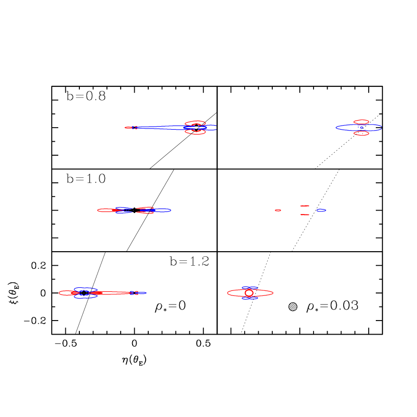
Figure 6.— Contours of constant fractional deviation, $\delta$, from the single-lens magnification for a point-source (left panels) and source with radius $\rho_{*}=0.03$ (right panels), as a function of source position $(\eta,\xi)$, in units of the Einstein ring radius, $\theta_{E}$, for mass ratio $q=10^{-4}$ and dimensionless separations $b=0.8,1.0,1.2$. The contours are the same as in Figure 2. The light curves arising from the sample trajectories (solid and dotted straight lines) are shown in Figure 7.

Figure 7.— The fractional deviation, $\delta$, from the single-lens light curve as function of time from the peak of the single lens light curve, $t_{0}$, in units of the Einstein ring crossing time $t_{E}$, for the trajectories shown in Figure 7. The solid line is for a point-source, and the dotted lines are for a source of radius $\rho_{*}=0.03$.

Figure 8.— The detection efficiency $\epsilon$ as a function of the dimensionless separation of the binary, $b$, for three different mass ratios $q$ and three events with different minimum impact parameter ${u_{\rm min}}$. The solid line is $\epsilon$ for a point-source and a detection criterion $\Delta\chi^{2}>225$; the dotted line is $\epsilon$ using the same detection criterion for a source of radius $\rho_{*}=0.03$. It is assumed that the events are sampled uniformly with $2\%$ photometry at the rate $t_{E}/200$ from alert to $t_{E}$.

6. Finite Source Effects

The calculations in § 5 implicitly assumed that the microlensed source was point-like, so that the magnification of the source is infinite at the caustics. The magnification $A_{\rm fs}$ of a source with finite size is given by the integral of the point-source magnification over the face of the star,

$$A_{\rm fs}(t)={{\int{\rm d}^{2}r\,A(t;{\bf{r}})I({\bf{r}})}\over{\int{\rm d}^{2}r\,I({\bf{r}})}}~{},$$ (11)

and is equivalent to the intensity-weighted area of the images (numerator) divided by the intensity-weighted area of the unlensed source (denominator). Here $I({\bf{r}})$ is the intensity profile of the source. The finite size of the source smoothes and broadens the discontinuous jumps in magnification near caustics by an amount that depends on the angular size of the source, $\theta_{*}$, in units of $\theta_{E}$,

$$\rho_{*}\equiv{\theta_{*}\over\theta_{E}}={R_{*}\over R_{E}}{{D_{\rm OL}}\over{D_{\rm OS}}}=0.03\left({M\over 0.2M_{\odot}}\right)^{1/2}\left(R_{*}\over 10R_{\odot}\right)~{},$$ (12)

where $R_{*}$ is the physical size of the star. For the scaling relation on the right of equation (12), a lens distance of ${D_{\rm OL}}=6~{}{\rm kpc}$ and a source distance of ${D_{\rm OS}}=8~{}{\rm kpc}$ has been assumed. For a given $\rho_{*}$, uniform sources ($I={\rm constant}$) will have a larger effect on the magnification than limb-darkened sources. Since we are interested primarily in the magnitude of the effect that finite sources will have on the detection efficiency, we will assume a (less-realistic) uniform source profile, which also increases computational speed.

Since the caustic of a point lens is a single point at the center of the lens ($u=0$), the magnification of a finite source will differ from that of a point source only when the source approaches the center of the lens, ${u_{\rm min}}\sim\rho_{*}$. For typical sources and lenses, $\rho_{*}\ll 1$ (c.f. equation (12)), so that for single lenses finite source effects are noticeable only in high magnification events (${u_{\rm min}}\ll 1$), for which $A\sim u^{-1}$ (equation (2)). Assuming a uniform source, the single lens magnification can be found analytically in this limit (Schneider, Ehlers, & Falco (1992)),

$$A_{\rm fs,0}(t)=A_{0}(t){\cal{B}}[z(t)],$$ (13)

where

$${\cal{B}}(z)=\cases{{4\over\pi}E(z)&$z\leq 1$\cr{4\over\pi}z\left[E(1/z)-(1-z^{-2})K(1/z)\right]&$z\geq 1$\cr}~{}.$$ (14)

Here $K$ and $E$ are the complete elliptic integrals of the first and second kind, and $z\equiv u/\rho_{*}$.

For a binary lens, the finite size of the source affects the magnification whenever the source approaches a caustic or, more precisely, wherever the second derivative of the magnification is large. As can be seen in Figure 2, for binaries with $q\sim 1$ much of the region inside the Einstein ring satisfies this condition: caustic approaches and crossings will be common. On the other hand, the results of § 5.1 indicate that caustic crossings make up only a small fraction of all detectable events for binaries with mass ratios consistent with planetary systems ($q{{}_{<}\atop{}^{{}^{\sim}}}10^{-2}$). Nevertheless, as can be seen from Figure 2, in order to produce a detectable event trajectories must pass close to caustics, where the gradient of the magnification is large and finite source effects are non-negligible. Finite source magnifications for binary lenses cannot be found analytically. Numerical integration of the point source magnification over the face of the star is difficult, as the divergent magnification near caustics causes the results to depend critically on the integration grid size. A more robust method is to compute the total area of all images and then divide by this area by that of the source to find the magnification of the finite source at that position. Numerous methods have been suggested; we will integrate over the boundary of the images (Kayser & Schramm (1988); Gould & Gaucherel (1997); Dominik (1998)). For alternative methods, see Bennett & Rhie (1996), Wambsganss (1997), and Griest & Safizadeh (1998).

What is relevant to this discussion is not the difference between the finite source and point source magnification, but the effects of finite source size on the determination of the detection efficiency $\epsilon$. For nearly equal-mass binaries $(q{{}_{>}\atop{}^{{}^{\sim}}}10^{-1})$, the magnification may be altered considerably by finite source effects without substantially altering $\epsilon$. This can be seen by comparing the size of the deviations ($\delta$) in the $q=1.0$ and $q=10^{-1}$ panels of Figure 2 to the size of a large source ($\rho_{*}=0.03$). For mass ratios as small as $q{{}_{<}\atop{}^{{}^{\sim}}}10^{-3}$, however, the size of the $\delta$ structures is comparable to that of a large source, and finite source effects are important to a proper determination of the detection efficiency $\epsilon$. Roughly speaking, finite source effects become important whenever the source size becomes comparable to the Einstein ring of the companion, $\theta_{*}{{}_{>}\atop{}^{{}^{\sim}}}\theta_{p}=q^{1/2}\theta_{E}$, or,

$$\rho_{*}\gtrsim q^{1/2}.$$ (15)

This criterion is satisfied at $\rho_{*}\simeq 0.1$ for $q\simeq 10^{-2}$, whereas for $q\sim 10^{-3}$ source sizes $\rho_{*}{{}_{>}\atop{}^{{}^{\sim}}}0.03$ will begin to seriously affect $\epsilon$. Since the largest sources routinely monitored in the Galactic bulge are clump giants, with $\rho\simeq 0.03$, finite source effects will be negligible for $q>10^{-3}$, but must be considered for smaller mass ratios.

Although the magnitude of the perturbation will always be suppressed in the presence of a finite source, it will also be broadened. Finite sources thus have competing effects on the detection efficiency $\epsilon$: $\epsilon$ is decreased because previously significant deviations are suppressed below the detection threshold, but increased for those trajectories for which the limb of the star grazes a caustic (or high magnification area) yielding a significant deviation where no significant deviation would have occurred for a point source. The net result of these two competing effects will depend on the specific value of $q$ and $b$.

Contours of constant fractional deviation $\delta$ of a binary from a single lens magnification, are illustrated in Figure 6 for both a point source and a finite source. We choose $\rho_{*}=0.03$, a relatively large source, and $q=10^{-4}$, the smallest mass ratio we consider, in order to present a scenario in which the source size will have an extreme effect. For the finite-source cases, the fractional deviation is computed with respect to a finite-source point-lens magnification, as given by equation (13). Figure 6 clearly demonstrates that, for this mass ratio and source size, the differences between the point and finite source magnification are dramatic. Both the shape and size of the $\delta$-contours are altered considerably.

As can be seen from Figure 6, planetary perturbations with $b<1$ are qualitatively different than those with $b>1$ (Gould & Loeb 1992; Gaudi & Gould 1997; Wambsganss 1997). Consider the case $b=0.8$: the perturbation is substantially depressed by the finite source and the $\delta=5\%$ contours have nearly disappeared. This is because, for $b<1$, regions of constant positive and negative deviation are closely spaced and of nearly equal area so that the smoothing induced by a large source tends to cause a cancellation leaving a deviation that is nearly zero (Bennett & Rhie (1996); Gould & Gaucherel (1997)). The effect is even more prominent for $b\sim 1$, where the regions of positive and negative deviation are especially closely spaced (Bennett & Rhie 1996). Obviously, for these two parameter combinations, the planet is unlikely to be detected and $\epsilon\rightarrow 0$. For $b>1$, regions of positive deviation encompass considerably more area than those of negative deviation (at a fixed value of $|\delta|{{}_{>}\atop{}^{{}^{\sim}}}5\%$), and the cancellation is less dramatic. As a result, $\epsilon(b>1)$ will be less affected by finite sources than $\epsilon(b\leq 1)$. In both cases, the perturbations caused by the central caustic (near $\zeta=0,\eta=0$) have dropped below $\delta=1\%$. Central caustics are an important channel to planet detection in high magnification events; detection efficiencies for these events will be highly sensitive to $\rho_{*}$ (Griest & Safizadeh (1998)). Fortunately, this is a class of events for which $\rho_{*}$ can often be measured.

In Figure 7, the light curves resulting from the trajectories shown in Figure 6 are displayed. The trajectories were chosen to create a significant point source fractional deviation, but are otherwise representative. Dramatic cancellation can be seen in the light curves for $b=0.8$ and $b=1.0$. For $b=1.2$, the deviation is substantially suppressed but is also broader. For photometry of sufficient precision, the detection efficiency $\epsilon$ for this parameter combination will actually be increased.

$u_{min}$	q	Point Source	$\rho=0.003$
0.1	0.01	$94.1\%$	91.3
	0.001	29.3	16.9
	0.0001	1.6	0.4
0.3	0.01	59.1	58.8
	0.001	13.8	15.0
	0.0001	4.9	0.5
0.5	0.01	34.3	34.9
	0.001	11.3	8.9
	0.0001	0.7	0.4

Table 2 Lensing Zone Detection Efficiencies ${\bar{\epsilon}}_{\rm LZ}(q)$, $\Delta\chi^{2}_{\rm thresh}=225$: Finite Source

To make a quantitative comparison, we have calculated $\epsilon$ in the same manner and for the same parameters as in § 5.1, but now compare the simulated light curves to the best-fit finite source binary light curves with $\rho_{*}=0.03$. The results with a detection criterion $\Delta\chi^{2}_{\rm thresh}=225$ are shown in Figure 8, along with the corresponding point source efficiencies from Figure 5. In agreement with the estimate from equation (15), the detection efficiency $\epsilon$ for $q=10^{-2}$ companions is hardly affected. For $q=10^{-3}$ and separations $b<1$, $\epsilon$ is similar to or smaller than finite source efficiencies, but for wider separations $b>1$, $\epsilon$ can be either somewhat smaller or somewhat larger due to the finite source size. The difference is dramatic for $q=10^{-4}$: source sizes corresponding to bulge giants always yield efficiencies ${{}_{<}\atop{}^{{}^{\sim}}}1\%$. As in § 5.1, we calculate lensing zone efficiencies ${\bar{\epsilon}}_{\rm LZ}$ (equation (10)); the results are shown in Table 6. We conclude that finite source sizes have negligible effect on $\epsilon$ for $q{{}_{>}\atop{}^{{}^{\sim}}}10^{-2}$, but sources as large as bulge giants ($\rho_{*}\simeq 0.03$) can have a dramatic effect for smaller companions, either increasing or decreasing $\epsilon$ ($q\simeq 10^{-3}$), or wiping out the detection efficiency completely $(q{{}_{<}\atop{}^{{}^{\sim}}}10^{-4})$.

Unfortunately, for individual events, the value of $\rho_{*}$ is very poorly constrained. While it is possible to estimate the physical size of the source from its color and magnitude, this cannot be translated to the dimensionless projected size $\rho_{*}$ if the value of $\theta_{E}$ remains unknown. The detection efficiency $\epsilon$ for most events could be in error therefore by many tens of percent (c.f. Figure 8 and Table 6). We discuss method of dealing with this difficulty in § 8.2.

Figure 9.— Ratio of blended $\delta_{B}$ to true fractional deviation $\delta$, as a function of impact parameter $u$ for three different blend fractions, $f_{B}$. Microlensing events are generally alerted when $u<1$.

Figure 10.— Left panels: The difference in $\chi^{2}$ between a point-lens fit with no blending and one with the blend fraction held fixed at $f_{B}$, for observations from alert ($A=1.54$) until $t=t_{E}$ (dotted line) and from alert until $t=3t_{E}$ (solid line). The effect of improving the photometric precision by a factor two while monitoring to $t=3t_{E}$ is also shown (long-dashed line). Right panels: The ratio of the fitted value of $u_{min}$ to the true value of $u_{min}$ as a function of the blend fraction. Line types are the same as the left panels; the long-dashed line is coincident with the solid line.

Figure 11.— The detection efficiency $\epsilon$ as a function of the dimensionless separation of the binary, $b$, for mass ratio $q=10^{-2}$ and four different blend fractions $f_{B}$ for an event with $2\%$ photometry, uniform sampling from alert until $t_{E}$ at the rate $t_{E}/200$, and minimum impact parameter ${u_{\rm min}}=0.5$.

7. Blending

A microlensing event is blended whenever unresolved, unlensed background light contributes significantly to the observed baseline flux of the source star (i.e. $f_{B}\neq 0$). From equation (1), the observed magnification in the presence of blending, $A_{B}$, is related to the true magnification by,

$$A_{B}=(1+f_{B})^{-1}(A+f_{B})~{},$$ (16)

where $f_{B}$ is the ratio of the blend flux to the true lensed source flux.

Blending will have two effects on the detection efficiency. The first is a suppression of the deviation caused by the binary. From equation (16) and equation (1), it is straightforward to show that the fractional deviation in the presence of a blend, $\delta_{B}$, is related to the true fractional deviation by,

$$\delta_{B}=\delta\left({1+{f_{B}\over A_{0}}}\right)^{-1}~{}.$$ (17)

As before, $A_{0}$ is the magnification of the best-fit PSPL light curve. Note that equation (17) applies to any anomaly that produces a deviation from the standard PSPL light curve, including parallax, binary source, and finite source effects. Since $A_{0}$ is a function of time, the magnitude of the suppression will also be a function of time, such that deviations occurring closer to the peak ($u\sim{u_{\rm min}}$) will be less suppressed than those occurring near the beginning and end of the event. Figure 9 shows the ratio $\delta_{B}/\delta$ as a function of the angular separation $u$ of the lens and source, for three values of $f_{B}$ corresponding to relatively mild blending, $f_{B}<1$. Anomalies occurring near the peak of high magnification events ($u\sim 0$) will be only slightly suppressed (Griest & Safizadeh (1998)), while repeating events caused by wide binaries (Di Stefano & Mao 1996; Di Stefano & Scalzo 1999b) can be suppressed by as much as $(1+f_{B})^{-1}$. Overall, the amplitude of the suppression for mild blending is relatively small, $\delta_{B}/\delta\leq(1+f_{B})^{-1}$, and thus will not have a large effect on the detection efficiencies for binaries with mass ratios $q\geq 10^{-2}$ for which the fractional deviations are usually large. For mass ratios consistent with planets, $q\leq 10^{-3}$, however, a substantial fraction of detected events will have maximum fractional deviation $\delta_{\rm max}{{}_{<}\atop{}^{{}^{\sim}}}0.1$ so that even a suppression of $\sim 0.5$ can have a significant effect on planetary detection efficiencies.

The second effect that blending has on detection efficiencies is to alter the presumed distribution of ${u_{\rm min}}$ in observed events. The intrinsic distribution of ${u_{\rm min}}$ is flat up to the magnification threshold set for detection by the survey teams (e.g., $A>1.34$ corresponds to ${u_{\rm min}}<1$). This threshold is calculated in real time near the beginning of the event when a robust determination of blending is not possible. Consequently, the magnification of the event at any time is assumed to be the total flux divided by the baseline flux, $A_{B}=(1+f_{B})^{-1}(A+f_{B})$, which is less than the true magnification $A$ for all non-zero blending values. Thus, in the presence of blending, an event will require a larger magnification and thus smaller intrinsic ${u_{\rm min}}$ in order to pass the detection criterion, which is per force applied to the observed quantity $A_{B}$ (see Alcock et al. 1997a for an example and discussion). Since the intrinsic detection efficiency is larger for smaller impact parameters (see § 5.1 and Figure 5), the blended event will be more sensitive to the presence of planets than would be calculated for a ${u_{\rm min}}$ based on the (erroneous) assumption that $f_{B}=0$. Blending thus affects binary detection efficiency in two competing ways: the efficiency is decreased by suppressing the amplitude of observed deviations, while at the same time it is increased due to the skewing of the observed ${u_{\rm min}}$ distribution to smaller values. The net effect on the detection efficiencies will depend on the values of $b$ and $q$ and vary on an event-by-event basis.

Clearly, blending must be considered when calculating binary and planetary detection efficiencies. Since blending effects are relatively easy to quantify, this poses no serious complication as long as the blending parameter, $f_{B}$, can be accurately determined for individual events. Unfortunately, as discussed by Woźniak & Paczynksi (1997), blending can be extremely difficult to determine for individual observed light curves, due to the serious correlations in the parameters $F_{0},t_{E},{u_{\rm min}}$ and $f_{B}$ in the presence of blending. The degeneracy is especially severe in two regimes. In the ‘spike’ regime, defined by $f_{B}\gg 1$ and ${u_{\rm min}}\ll 1$, $t_{E}$ and ${u_{\rm min}}$ cannot be measured separately and only the degenerate combination $t_{E}/{u_{\rm min}}$ is measurable (Gould (1996)). This regime is most important in severely crowded fields, such as those towards M31. The second regime, defined by large impact parameter (${u_{\rm min}}{{}_{>}\atop{}^{{}^{\sim}}}0.5$) events with modest blending $f_{B}<1$, is more common in bulge fields, and thus the focus of our current attention.

In order to illustrate the difficulty in quantifying the fraction of blended light, we calculate the range of allowed values inferred for $f_{B}$ from fits to our fiducial simulated light curves (i.e., observations from alert until $t_{E}$, $2\%$ errors, and no blending). Fixing $f_{B}$ at some value, we find the best fit to a point-lens model allowing the parameters ${u_{\rm min}},t_{E},t_{0},$ and $F_{0}$ to vary. We then compute $\Delta\chi^{2}$ between this fit and that assuming $f_{B}=0$. The resulting $\Delta\chi^{2}$ as a function of $f_{B}$ is shown in Figure 10. For ${u_{\rm min}}=0.1$ and ${u_{\rm min}}=0.3$, the degeneracy is not severe; the $3\sigma$ allowed ranges in $f_{B}$ are $f_{B}\leq 0.125$ and $f_{B}\leq 0.45$, respectively. For ${u_{\rm min}}=0.5$, the blend fraction is almost completely unconstrained because for large ${u_{\rm min}}$ events constraints on blending arise mostly from the combination of information from the wings ($|t-t_{0}|\sim t_{E}$) of the event and the baseline ($|t-t_{0}|\gg t_{E}$). Thus, without a baseline measurement, the value of $F_{0}$ can be arbitrarily adjusted to compensate for large values of $f_{B}$ without significantly affecting the fit. With this in mind, we have also computed the same $\Delta\chi^{2}$ statistic for a simulated light curve with observations from alert until $3t_{E}$. Here the blending is much better constrained, $f_{B}\leq 0.27$, with additional improvement if the errors are reduced by half, in which case $f_{B}\leq 0.15$. Since the majority of the constraint comes from sampling the wings and baseline of the light curve, it would be more efficient for monitoring teams to concentrate on more, rather than better, measurements.

The right panels of Figure 10 demonstrate how an inaccurately-determined blend fraction can affect the determination of ${u_{\rm min}}$ and thus the detection efficiency $\epsilon$. Here we show the ratio between the value of ${u_{\rm min}}$ determined by assuming a constant blend fraction $f_{B}$, $u_{\rm min,f}$, and the true value ${u_{\rm min}}$. The value of ${u_{\rm min}}$ deduced for blend fractions between $f_{B}=0$ to $f_{B}=0.4$ can vary by nearly $50\%$ resulting in quite different inferred detection efficiencies (c.f. Figure 5). To quantify this, we have calculated $\epsilon$ as a function of $f_{B}$ for an extreme example, ${u_{\rm min}}=0.5$ and observations from alert until $1t_{E}$. The procedure for calculating $\epsilon$ is the same, except now $f_{B}$ is fixed at an assumed value and $F_{0}$ is included as a free parameter in both the single lens and binary lens fits. The results are shown in Figure 11, where we plot $\epsilon(q=10^{-2})$ as a function of $b$ for $f_{B}=0$ (same as Figure 5), $0.2$, $0.4$, and $0.6$. Recall that all these blend fractions are statistically indistinguishable for this light curve. The differences in $\epsilon$ are dramatic. The suppression of binary anomalies induced by blending of $f_{B}=0$ and $0.2$ causes a drop in detection efficiency for separations $b{{}_{<}\atop{}^{{}^{\sim}}}0.6$ and $b{{}_{>}\atop{}^{{}^{\sim}}}1.6$. Inside the Lensing Zone, however, the net effect is a dramatic increase in $\epsilon$ due to the lower value of ${u_{\rm min}}$ required to produce the observed light curve for increasing $f_{B}$. This can be appreciated best by examination of Table 7, which tabulates ${\bar{\epsilon}}_{\rm LZ}$ as a function of $f_{B}$. To the extent that these values of $f_{B}$ cannot be distinguished from one another by the light curve alone, they are all equally likely, and thus $\epsilon$ can be quite uncertain.

$f_{B}$	$u_{min,f}$	${\bar{\epsilon}}_{\rm LZ},\Delta\chi^{2}_{\rm thresh}=225$
0.0	0.50	34.3%
0.1	0.44	32.7
0.2	0.40	37.2
0.3	0.34	39.6
0.4	0.28	41.7
0.5	0.19	56.8
0.6	0.02	52.7

Table 3 Lensing Zone Detection Efficiencies ${\bar{\epsilon}}_{\rm LZ}(q=10^{-2})$: Blending

Blending can give rise to a serious uncertainty in derived detection efficiencies but, unlike finite source size, the blend fraction can be determined with sufficient accuracy for most events. To do so, however, requires precise measurements by the monitoring teams during the wings of the event and at baseline. Without a reasonable quantification of the blend fraction, the detection efficiency of individual events will be very uncertain.

8. Application to Real Data

In previous sections, we used artificial data to explore several effects that can influence significantly the determination of the detection efficiency $\epsilon$ of individual light curves, including detection criteria (§ 5.1), finite source size (§ 6), and blending (§ 7). These effects are often difficult to quantify in real data, for which sampling and photometric precision is likely to vary on an event-by-event basis, and with observing conditions and microlensing phase for individual events. Furthermore, real-time observational decisions may alter (increase) the sampling of clearly anomalous events from that of apparently non-anomalous PSPL events.

8.1. Variable Sampling and Photometric Precision

Since the algorithm we presented in § 5 uses the actual light curve, and thus the actual sampling and photometric uncertainties associated with each observed event, irregular sampling and variable precision are taken into account explicitly in the determination of the detection efficiency $\epsilon$. The efficiencies based on artificial data presented in previous sections to illustrate general principles will not be strictly applicable to real microlensing events, for which weather and other considerations prevent continuous monitoring with a sampling of $t_{E}/200$. In general, the effect of reduced or incomplete sampling will be to lower detection efficiencies. For extremely long events, or those (including very short) events alerted post-peak by the survey teams, substantial portions of the light curve will have no (dense) monitoring at all, and the effects on the detection efficiency can be quite devastating. In such partially-monitored light curves, the PSPL fit parameters (${u_{\rm min}},t_{E},t_{0},F_{0}$ and $f_{B}$) will be very uncertain, and in extreme cases almost completely unconstrained. Since the detection efficiency depends on these parameters, the resulting uncertainty in $\epsilon$ will be quite large. Unless additional information is available (e.g. from the survey teams) to constrain the fit, these data will add almost nothing to our knowledge of the abundance of planets since their detection efficiency cannot be reliably quantified.

For Gaussian, uncorrelated errors, the $\chi^{2}$ statistic can be used as a measure of goodness-of-fit. Real measurement uncertainties are seldom truly Gaussian, especially in crowded microlensing fields where systematic effects associated with seeing, scattered light, and detector characteristics become increasingly important. Uncertainties on individual data points are often taken to be the formal errors reported by the PSF-fitting algorithms of photometric reduction packages like DoPhot (Schechter, Mateo, & Saha (1993)), which often underestimate the true scatter (Albrow et al. (1998)). Image subtraction techniques (Tomaney & Crotts (1996); Alard & Lupton (1998)) may alleviate some of these difficulties, but for the moment are too cumbersome and slow to implement for multi-site, real-time reduction of large fields and thus have not yet been implemented by monitoring teams. An empirical correction to account for the correlation of measured photometric magnitude with the FWHM of the point spread function often results in a more Gaussian error distribution whose average magnitude corresponds more closely to the formal DoPhot-reported error (Naber, private communication; Albrow et al. (1999)). As long as the detection criterion $\Delta\chi^{2}_{\rm thresh}$ is maintained at a suitably high value (§ 5), the exact error distribution is likely to have little effect on the computed efficiency $\epsilon$. Remaining doubts can be assuaged by attaching the observed error distribution derived from constant stars to artificially generated PSPL light curves to calibrate both the ‘false alarm rate’ and efficiency of true detections with a given $\Delta\chi^{2}_{\rm thresh}$ criterion.

8.2. Finite Source Effects

Finite source effects pose a significant challenge to the robust determination of the detection efficiency $\epsilon$ because the dimensionless source size, $\rho_{*}$ is unknown a priori. As we have shown in § 5, the finite size of the source should have negligible effect on $\epsilon$ for $q{{}_{>}\atop{}^{{}^{\sim}}}10^{-2}$ but can have a significant effect for $q{{}_{<}\atop{}^{{}^{\sim}}}10^{-3}$. Thus, without additional information about $\rho_{*}$, $\epsilon$ can be determined robustly only for $q{{}_{>}\atop{}^{{}^{\sim}}}10^{-2}$, which is unsatisfactory for microlensing monitoring programs whose primary goal is to learn about small mass-ratio systems. A first-order estimate for $\rho_{*}$ could be obtained by measuring the angular size of the source, $\theta_{*}$, and assuming that the relative proper motion of the lens, $\mu=v_{\perp}/{D_{\rm OL}}$, is equal to the mean relative proper motion $\langle\mu\rangle$ for all lenses toward the bulge. The dimensionless size of the source would then be given by

$$\rho_{*}\approx{\theta_{*}\over\langle\mu\rangle\,t_{E}}~{}.$$ (18)

The angular size of the source can be estimated by its color and magnitude, or by obtaining a precise spectral type through more resource-intensive spectroscopy. Unfortunately, the value of $\langle\mu\rangle$ depends on the assumed velocity and spatial distribution of the lenses. Moreover, even within a given model, the distribution of $\mu$ is wide, having a variance of a factor of $\sim 3$ and long tails toward higher and lower values (Han & Gould (1995)). The true value of $\mu$ thus could differ substantially from $\langle\mu\rangle$, leading to a large error in $\epsilon$ for individual events. When averaged over many events, these errors should approximately cancel, but current monitoring programs are very far from this regime, especially for anomalous events.

A somewhat better estimate for the effect of $\rho_{*}$ on detection efficiencies could be made as follows. Assume that an event has measured time scale $t_{E}$ and angular source size $\theta_{*}$. For an assumed model of lens distances and velocities, the expected distribution of proper motions, ${\cal G}_{i}(\mu)$, can be computed. The individual detection efficiency can then be approximated as,

$$\epsilon_{i}(b,q)=\int_{\mu_{\rm min}}^{\mu_{\rm max}}{\rm d}\mu\,\epsilon_{i}(b,q;\rho_{*}){\cal G}_{i}(\mu)~{},$$ (19)

where $\rho_{*}={\theta_{*}/\mu t_{E}}$, $\mu_{\rm max}$ is the maximum proper motion allowed by the observed light curve, and $\mu_{\rm min}$ is some reasonable lower limit. This model-dependent estimate of the detection efficiency should be more accurate whenever finite source effects are large, but it is time consuming to compute because $\epsilon(b,q)$ must be determined for many $\rho_{*}$.

Ideally, one would like to determine $\rho_{*}$ directly for each individual lens. This can be done by measuring $\mu$ from single-color light curves for only $\sim 5\%$ of events (Gould (1994), Witt (1995)), namely those with high peak magnification. With both optical and infrared photometry, $\rho_{*}$ could be determined for approximately twice as many events (Gould & Welch (1996); Witt (1995)). If the lens is luminous, one could measure the proper motion of the lens directly using accurate astrometry and a high resolution instrument, such as HST (Gaudi & Gould (1997)). This will not be possible for all events, however, and requires a long temporal baseline. The angular Einstein ring radius $\theta_{\rm E}$ can be determined directly by measuring the centroid shift of the two unresolved images created by the lens. As the lens passes across the line of sight to the source, these two images move and change magnification. The centroid of these two images traces out an ellipse who size is $\sim\theta_{E}$ (Walker (1995)), thus requiring an an astrometric accuracy considerably smaller than 1 mas. Preliminary studies have shown that SIM, with its planned $4\mu{\rm as}$ accuracy, should be able to measure $\theta_{E}$ reliably for almost all known microlenses toward the galactic bulge (Boden et al. 1998a ; Jeong, Han & Park (1999); Dominik & Sahu (1999); Gould & Salim (1999)). Ground-based interferometers currently being developed, such as the Keck Testbed Interferometer, should be able to measure $\theta_{E}$ for a smaller, but substantial, fraction of events (Boden et al. 1998a ). Measurements of this kind would require coordination and cooperation between microlensing and astrometric communities, but the results would be well worth the effort.

In summary, if microlensing monitoring teams can make use of other resources, such as HST and SIM, the best method of dealing with finite source size effects is simply to measure the dimensionless source size $\rho_{*}$ for each individual event directly. In the absence of these options, the effect of finite source size on $\epsilon$ must rely on statistical and model-dependent estimates of the distribution of $\rho_{*}$.

8.3. Blending

As discussed in § 7, the accurate determination of the blending, $f_{B}$, in individual light curves is essential to the accurate determination of the detection efficiency. Precise measurements during the wings of the event and at baseline can allow the quantification of $f_{B}$, but may not always be possible: bad weather may prevent wing measurements in some events and the faintness of the source star may preclude precise baseline measurements in others. Improved or alternate methods of quantifying blending would be beneficial; several have already been suggested.

Since the blending problem arises mainly because the PSFs of individual stars are blended together in crowded microlensing fields, simply improving the spatial resolution of the observations eliminates or reduces the blended light in most cases. The resolution needed is roughly that of HST (Han (1997)), for which only a modest use of resources is required. Nevertheless, even the resolution of HST will be insufficient to resolve any blended light that might arise from the lens itself or unresolved companions to the lens or source. Blending caused either by the lens or unrelated projected stars near the source or lens will generally cause a color shift in the combined light as the source is magnified during the course of the event (Buchalter & Kamionkowski (1996)). Since most stars in the bulge have nearly the same color, the color shift is expected to be small and difficult to measure. Alternatively, the blend fraction can be quantified by measuring the centroid shift of the blended PSF during the course of the event (Goldberg & Woźniak ; Goldberg (1998)). Blend fractions can be reliably determined in this way only for heavily blended, high-magnification events (Han, Jeong, & Kim (1998)) in which the centroid shift is prominent. Finally, improvement can be made through using image subtraction rather than the usual PSF-fitting photometry. Image subtraction reveals only the time-variable flux, $\Delta F=F_{0}[A(t)-1]$, so that constant sources of blended light are removed. Although image subtraction does not remove the correlations between fitted parameters that make blending problematic, it is useful since photometric uncertainties are generally near the photon noise limit (Tomaney & Crotts (1996); Alard & Lupton (1998)), which allows better discrimination between subtle differences in blended light curves.

8.4. Anomalous Events

If solar systems like our own are not atypical, dense, precise photometric monitoring will eventually result in the detection of anomalous events consistent with planetary perturbations. The algorithm of § 5 can be used to place direct limits on planetary systems in non-anomalous events and give meaning to the large number of null results now in hand, but what of the detection efficiency of events in which planetary anomalies are actually observed?

By the detection efficiency $\epsilon_{i}(b,q)$ of an anomalous event, we mean, by analogy with the definition for non-anomalous events given in § 4, the probability that a lensing companion with parameters $b,q$ would be detected in light curve $i$ (using the same $\Delta\chi^{2}_{\rm thresh}$ criterion) after integrating over source trajectory angles $\theta$. In principle, if the parameters $t_{0},t_{E},{u_{\rm min}},F_{0}$ and $f_{B}$ can be well-determined in a binary fit that meets the $\Delta\chi^{2}_{\rm thresh}$ criterion, $\epsilon(b,q)$ can be calculated in a manner similar to that presented in § 5. A PSPL light curve with these parameters can be generated with the actual sampling and photometric errors of the observed event and the method of § 5 applied for the $b,q$ combination that produced the best-fit ‘detected’ binary.

Several difficulties inherent to anomalous light curves must be addressed. First, for large mass ratio ($q{{}_{>}\atop{}^{{}^{\sim}}}10^{-2}$), the source trajectory $\theta$ may actually be constrained by the light curve itself, but in a way that is partially degenerate with other fitting parameters. Second, even for small mass ratios, i.e., true planetary anomalies, the parameters $t_{0},t_{E},{u_{\rm min}},F_{0}$ and $f_{B}$ may not be well-constrained, though of course this difficulty is present for non-anomalous events as well. Third, the anomaly, if large, may produce changes in magnification significant enough to alter the photometric precision obtained at the phase of the perturbation. Most planetary anomalies will have rather gentle changes in magnification (Figure 3) so that this effect may not be severe for $q{{}_{<}\atop{}^{{}^{\sim}}}10^{-3}$. Fourth, if detected real time, observer intervention may alter the photometric sampling in a way that is also phase-dependent (i.e. higher sampling after the anomaly detection than before). These last two possibilities present difficulties when integrating the corresponding PSPL light curve over source trajectory $\theta$, since the altered sampling and photometric errors will not correspond to the phase of actual anomalies for most choices of $\theta$.

One approach to handling this increased sampling at the phase of the anomaly is to resample the ‘post-anomaly’ portion of the light curve in a manner that is consistent with what would have been the sampling had the anomaly gone unnoticed. (Determining how to do this in the presence of weather and other observing facts-of-life may not be trivial). Both the initial test of binarity and the procedure to determine the detection efficiency would then be performed with the sparser, resampled light curve. The full dataset would be used only to refine the best-fit parameters. Alternatively, a Bayesian approach to analyzing the full dataset (anomalous and non-anomalous) could be employed, which addresses many of the special difficulties posed by anomalous events (Sackett 1999b ).

9. Conclusion

In this paper, we have presented and tested a method to calculate the detection efficiency of microlensing datasets to stellar and planetary lensing companions. This method is conceptually simple, direct, and not excessively time consuming. The final result, $\epsilon(b,q)$, conveniently summarizes the efficiency of a given dataset in revealing binary lensing systems with any mass ratio $q$ and dimensionless separation $b$. This efficiency can then be used to evaluate the likelihood that any given model of planetary systems would give rise to the observed dataset.

The algorithm that we have presented has several advantages. First, by working directly with measured light curves, it makes few assumptions, and explicitly takes into account the dependence of the efficiency on the sampling, photometric precision, monitoring duration, and impact parameter of the events. Second, it is computationally efficient, involving direct integration over only one unknown parameter, the angle of the trajectory. Finally, it is convenient, incorporating all information into one two-dimensional function, $\epsilon(b,q)$, which can then be used to evaluate the likelihood of any model of planetary systems.

Some caveats must be noted. First, the method assumes that the primary lensing parameters $t_{0},t_{E},{u_{\rm min}},F_{0}$ and $f_{B}$ are well-constrained by the light curve, while emphasizing that $\epsilon$ is poorly known in the absence of such constraints. Possible altered sampling and photometric precision of anomalous events may necessitate a resampling of the corresponding light curve or the assumption that the efficiency of anomalous events is equal to the average efficiency of the normal events. Resampling is not an efficient use of all the data, and for individual events the average efficiency of non-anomalous events is likely to be a rather poor proxy for $\epsilon_{i}$. Finally, the algorithm implicitly assumes that the efficiency is independent of the planetary system model (e.g., the effect of multiple planets is ignored).

We have also applied our method to artificial light curves in order to explore the dependence of binary detection efficiency on the impact parameter of the event, the choice of the detection criterion, neglecting to fit comparison binary curves separately, finite source effects, and blending. Our conclusions are as follows:

(1)

Most of the efficiency of microlensing datasets to detecting planetary anomalies results from non-caustic crossing events.

(2)

Detection efficiency is strongly dependent on the impact parameter ${u_{\rm min}}$ of the event. This implies that the integrated detection efficiency will depend strongly on the actual distribution of impact parameters of the monitored events.

(3)

For mass ratios $q\geq 10^{-2}$, the inferred detection efficiency $\epsilon$ is robust to changes in the detection criterion $\Delta\chi^{2}_{\rm thresh}$. For smaller mass ratios $q\sim 10^{-4}$ near the detection limit, different choices of $\Delta\chi^{2}_{\rm thresh}$ can lead to differences in $\epsilon$ of a factor of two.

(4)

In order to obtain accurate detection efficiencies, the binary lens light curve must be fit separately unless the mass ratio is small ($q{{}_{<}\atop{}^{{}^{\sim}}}10^{-3}$) and the deviations are well above the detection limit (which may be difficult to satisfy simultaneously).

(5)

Finite source effects are negligible for $q{{}_{>}\atop{}^{{}^{\sim}}}10^{-2}$, can either increase or decrease $\epsilon$ for $q\simeq 10^{-3}$, and can be devastating for $q{{}_{<}\atop{}^{{}^{\sim}}}10^{-4}$, at least for the large dimensionless source sizes ($\rho{{}_{>}\atop{}^{{}^{\sim}}}0.03$) that are typical of bulge giants.

(6)

The detection efficiency is very sensitive to the fraction of blended light, primarily due to item (2) above; higher blend fractions imply smaller impact parameters for detection, and smaller impact parameters have higher intrinsic detection efficiencies. This fact, combined with the degeneracy in the blend fraction that exists between poorly/inaccurately sampled blended light curves means that monitoring teams should make every effort to quantify the blend fractions in every monitored light curve.

The final result of applying this method to an observed data set is the integrated detection efficiency, $\epsilon(b,q)$. This result should be regarded as a primary outcome of microlensing monitoring teams conducting planet searches; it incorporates all the information from the observations, and is essential for establishing any conclusions about the abundance and nature of Galactic planetary systems.

References

- Alard & Lupton (1998) Alard, C., & Lupton, R.H. 1998, ApJ, 503, 325
- Albrow et al. (1997) Albrow, M., et al. 1997, in Variable Stars and the Astrophysical Returns of Microlensing Surveys, ed. R. Ferlet, J.-P. Maillard, & B. Raban (Gif-sur-Yvette:Editions Fronti res), 135
- Albrow et al. (1998) Albrow, M., et al. 1998, ApJ, 509, 687
- Albrow et al. (1999) Albrow, M., et al. 1999, in preparation
- Alcock et al. (1993) Alcock, C., et al. 1993, Nature, 365, 621
- Alcock et al. (1995) Alcock, C., et al. 1995, ApJ, 447 133
- (7) Alcock, C., et al. 1997a, ApJ, 479, 119
- (8) Alcock, C., et al. 1997b, ApJ, 486, 697
- (9) Alcock, C., et al. 1997c, ApJ, 491, L11
- (10) Alcock, C., et al. 1997d, ApJ, 491, 436
- Angel & Woolf (1997) Angel, R., & Woolf, N. 1997, ApJ, 475, 373
- Aubourg et al. (1993) Aubourg, E., et al. 1993, Nature, 365, 623
- Bennett & Rhie (1996) Bennett, D. & Rhie, S. H. 1996, ApJ, 472, 660
- (14) Boden, A., et al. 1998a, ApJ, 502, 538
- (15) Boden, A., et al. 1998b, ApJ, 504, L39
- Bolatto & Falco (1993) Bolatto, A., & Falco, E. 1993, ApJ, 436, 112
- Borucki et al. (1997) Borucki, W. J., et al. 1997, in Planets Beyond the Solar System and the Next Generation of Space Missions, ed. D. Soderblom (San Francisco:Astronomical Society of the Pacific), 119
- Buchalter & Kamionkowski (1996) Buchaleter, A., & Kamionkowski, M. 1996, ApJ, 469, 676
- Butler et al. (1996) Butler, R.P., et al. 1996, PASP, 108,500
- Cochran et al. (1997) Cochran, W.C., et al. 1997, ApJ, 483, 457
- Deeg et al. (1998) Deeg, H.J., et al. 1998, A&A, 338, 479
- Deleuil et al. (1997) Deleuil, M., et al. 1997, in Planets Beyond the Solar System and the Next Generation of Space Missions, ed. D. Soderblom (San Francisco:Astronomical Society of the Pacific), 259
- Di Stefano & Mao (1996) Di Stefano, R., & Mao, S. 1996, ApJ, 457, 93
- (24) Di Stefano, R., & Scalzo, R. 1999a, ApJ, 512, 564
- (25) Di Stefano, R., & Scalzo, R. 1999b, ApJ, 512, 579
- Dominik (1998) Dominik, M. 1998, A&A, 333L, 79
- Dominik (1999) Dominik, M. 1999, A&A, submitted.
- Dominik & Sahu (1999) Dominik, M., & Sahu, K. 1999, ApJ, submitted
- Gaudi (1998) Gaudi, B. S. 1998, ApJ, 506, 533
- Gaudi & Gould (1997) Gaudi, B. S., & Gould, A. 1997, ApJ, 486, 85
- Gaudi, Naber, & Sackett (1998) Gaudi, B. S., Naber, R. M., & Sackett, P. D. 1998, ApJ, 502, L33
- Goldberg (1998) Goldberg, D.M. 1998, ApJ, 498, 156
- (33) Goldberg, D.M., & Woźniak, P. 1998, Acta Astron., 48, 19
- Gould (1994) Gould, A. 1994, ApJ, 421, L71
- Gould (1996) Gould, A. 1996, ApJ, 470, 201
- Gould & Gaucherel (1997) Gould, A., & Gaucherel, C. 1997, ApJ, 477, 580
- Gould & Loeb (1992) Gould, A., & Loeb, A. 1992, ApJ, 396, 104
- Gould & Welch (1996) Gould, A., & Welch, D. 1996, ApJ, 464, 212
- Gould & Salim (1999) Gould, A., & Salim, S. 1999, ApJ, submitted
- Griest & Safizadeh (1998) Griest, K., & Safizadeh, N. 1998, ApJ, 500, 37
- Hale & Doyle (1994) Hale, A., & Doyle, L. 1994, Ap&SS, 212, 335
- Han (1997) Han, C. 1997, ApJ, 490, 51
- Han, Jeong, & Kim (1998) Han, C., Jeong, Y., & Kim, H.-I. 1998, ApJ, 507,102
- Han & Gould (1995) Han, C., & Gould, A. 1995, ApJ, 447, 53
- Jeong, Han & Park (1999) Jeong, Y., Han, C., & Park, S.-H. 1999, ApJ, 511, 569
- Kayser & Schramm (1988) Kayser, R., & Schramm, T. 1998, A&A, 191, 39
- Lindegren & Perryman (1996) Lindegren, L. & Perryman, M.A.C. 1996, A&AS, 116, 579
- Mao & Paczyński (1991) Mao, S., & Paczyński, B. 1991, ApJ, 374, 37
- Marcy & Butler (1998) Marcy, G.,& Butler, R. 1998, ARA&A, 36, 57
- Mayor & Queloz (1995) Mayor, M, & Queloz, D. 1995, Nature, 378, 355
- McMillan et al. (1993) McMillan, R.S., et al. 1993, ApJ, 403, 801
- Nelson & Angel (1998) Nelson, A. F., & Angel, J. R. P. 1998, ApJ, 500, 940
- Noyes et al. (1997) Noyes, R.W., et al. 1997, ApJ, 483, L111
- Paczyński (1986) Paczyński, B. 1986, ApJ, 304, 1
- Palanque-Delabrouille et al. (1998) Palanque-Delabrouille, N., et al. 1998, A&A, 332, 1
- Peale (1997) Peale, S. J. 1997, Icarus, 127, 269
- Press et al. (1992) Press, W.H., Flannery, B.P., Teukolsky, S.A., & Vetterling, W.T. 1992, Numerical Recipes (Cambridge: Cambridge Univ. Press)
- Renault et al. (1998) Renault, C., et al. 1998, A&A, 329, 522R
- Rhie et al. (1999) Rhie, S.H., et al. 1999, ApJ, submitted
- Sackett (1997) Sackett, P.D. 1997, Final Report of the ESO Working Group on the Detection of Extrasolar Planets, Appendix C (ESO Document: SPG-VLTI-97/002, and astro-ph/9709269)
- (61) Sackett, P.D. 1999a, in Planets outside the Solar System: theory and observations, eds. J.-M. Mariotti & D. Alloin, NATO-ASI Series, Kluwer. (astro-ph/9811269)
- (62) Sackett, P.D. 1999b, in preparation
- Schechter, Mateo, & Saha (1993) Schechter, P.L., Mateo, M., & Saha, A. 1993, PASP, 105, 1342
- Schneider, Ehlers, & Falco (1992) Schneider, P., Ehlers, J., & Falco, E.E. 1992, Gravitational Lenses (Berlin, Springer)
- Tomaney & Crotts (1996) Tomaney, A.B., & Crotts, A.P.S. 1996, AJ, 112, 2872
- Udalski et al. (1993) Udalski, A., et al. 1993, Acta Astron., 43, 289
- Udalski et al. (1997) Udalski, A., et al. 1997, Acta Astron., 47, 169
- Walker (1995) Walker, M.A. 1995, ApJ, 453, 37
- Wambsganss (1997) Wambsganss, J. 1997, MNRAS, 284, 172
- Witt (1990) Witt, H. 1990, A&A, 236, 311
- Witt (1995) Witt, H. 1995, ApJ, 449, 42
- Woolf & Angel (1998) Woolf, N., & Angel, R. 1998, ARA&A, 36, 507
- Woźniak & Paczyński (1997) Woźniak, P., & Paczyński, B. 1997, ApJ, 487, 55