SPREAD OF MATTER OVER A NEUTRON-STAR SURFACE DURING  DISK ACCRETION

Abstract

Disk accretion onto a slowly rotating neutron star with a weak magnetic field $H<3\times 10^{8}$ gauss is considered in a wide range of luminosities $1/100<L/L_{edd}<1,$ where $L_{edd}$ is the Eddington luminosity. We construct a theory for the deceleration of rotation and the spread of matter over the stellar surface in the shallow-water approximation. The rotation slows down due to friction against the dense underlying layers. The deceleration of Keplerian rotation and the energy release take place on the stellar surface in a latitudinal belt whose meridional width rises with increasing $L.$ The combined effect of centrifugal force and radiation pressure gives rise to two latitudinal rings of enhanced brightness which are symmetric around the equator in the upper and lower hemispheres. They lie near the edges of differentially rotating and radiating upper and lower belts. The bright rings shift from the equatorial zone to higher latitudes when the luminosity $L$ rises. The ring zones are characterized by a minimum surface density and, accordingly, by a maximum meridional spread velocity. At a low accretion rate and luminosity, the released energy is removed through the comptonization of low-frequency photons.

^∗ To appear in Astron. Lett., 1999, vol. 25, no. 5 (May issue).

Submitted 1998, October 15.

1 OVERALL PICTURE

In the Newtonian approximation, half of the gravitational energy is released in an extended disk during accretion onto a neutron star with a weak magnetic field. If the star rotates slowly, the other half of the energy must be released in the immediate vicinity of the star as the matter transfers from the disk onto the surface. This energy release is generally thought to occur in a narrow (both in radius and in latitude) boundary layer of the disk which is formed near the contact boundary between the disk and the star. The boundary layer is significant not only due to contribution to the luminosity of the compact object. It is important since the boundary-layer area is small compared to that of the disk, the layer’s emission is harder and must be observed in a different spectral range relative to the disk emission.

Accretion onto a neutron star differs in many ways from accretion onto a white dwarf. First, the percentage of energy which is released in the boundary layer can exceed appreciably $50\%$ because of the general-relativity effects (Sunyaev and Shakura 1986). The boundary-layer luminosity $L_{SL}$ is greater than the disk luminosity $L_{d}$ even for rapidly rotating neutron stars, but the ratio $L_{SL}/L_{d}$ decreases with the increasing angular velocity of the star (Sibgatullin and Sunyaev 1998). Second, at luminosities $L>L_{edd}/100\sim 10^{36}$ erg s${}^{-1},$ the local flux of radiative energy which is emitted from the boundary layer is of the order of the Eddington flux, i.e., the force of radiation pressure on an electron is of the order of the gravitational force acted on a proton. There are also other dissimilarities.

Most of the authors who considered disk accretion onto stars (Shakura and Sunyaev 1973; Lynden-Bell and Pringle 1974; Pringle and Savonije 1979; Papaloizou and Stanley 1986; Popham et al. 1993), white dwarfs (Tylenda 1981; Meyer and Meyer-Hofmeister 1989; Popham and Narayan 1995), and neutron stars (Shakura and Sunyaev 1988; Bisnovatyi-Kogan 1994) suggest that the accreting-plasma velocity decreases from the Keplerian velocity to the stellar rotation velocity through the turbulent friction between the differentially rotating layers of accreting matter within a thin boundary layer of the disk (see Fig. 1). In this case, $d\omega/dr>0$ in the boundary layer, the boundary-layer meridional extent is $R\theta_{bl}=R\sqrt{2T_{bl}/m_{p}}/v_{\varphi}^{k},$ and its height is $h_{bl}\simeq R(2T_{bl}/m_{p})/(v_{\varphi}^{k})^{2},$ where $R$ is the stellar radius, $T_{bl}$ is the boundary-layer temperature given in energy units, $m_{p}$ is the proton mass, and $v_{\varphi}^{k}$ is the Keplerian velocity at the radius $R$ (Shakura and Sunyaev 1988). The meaning of the geometrical quantities $h_{bl}$ and $\theta_{bl}$ is clear from Fig. 1. We see that in this approach, $h_{bl}$ is determined by the scale height in a gravity field with a free fall acceleration $g_{0}=\gamma M/R^{2}=$ $(v_{\varphi}^{k})^{2}/R.$ The boundary-layer meridional extent, $R\theta_{bl},$ is given by the same formula that is used to calculate the disk thickness, i.e., only the tangential component of the gravity force is taken into account. The thickness, $h_{bl},$ and the meridional extent turn out to be independent of latitude and accretion rate, respectively.

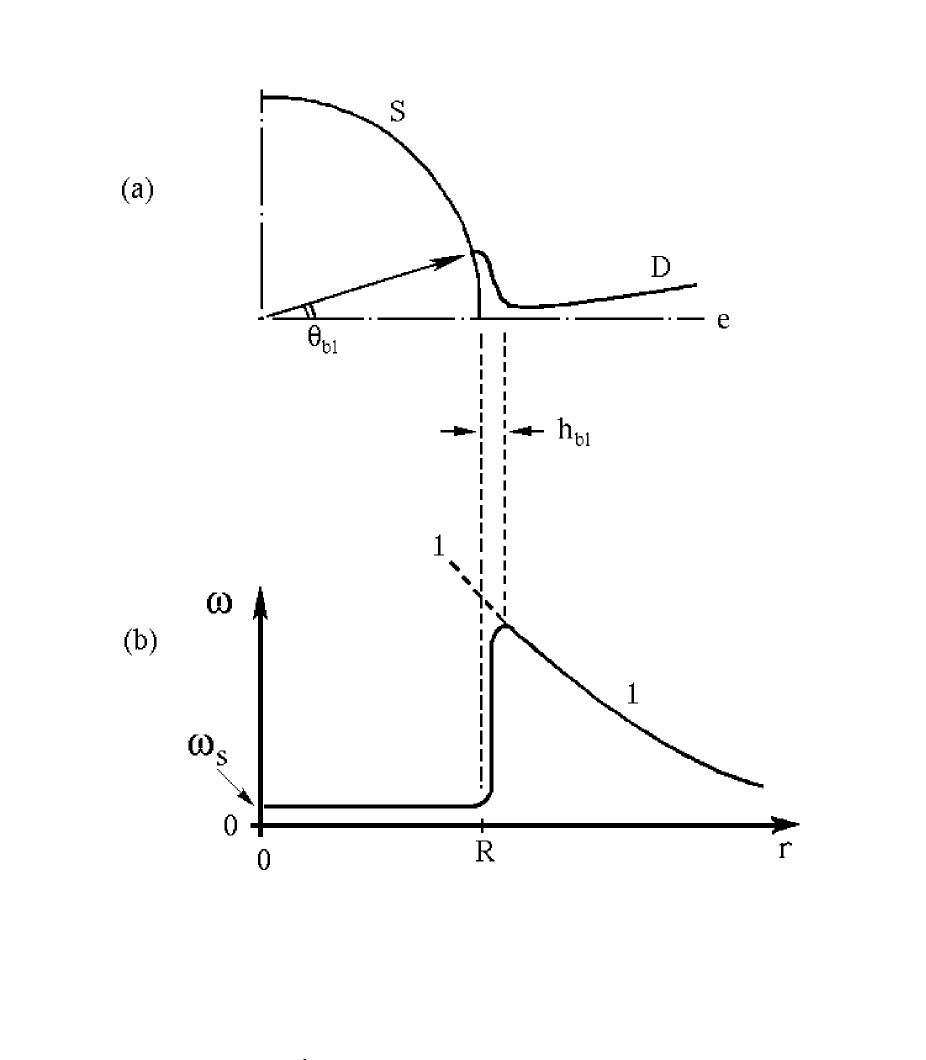
Figure 1: (a) Shape of the boundary layer in the standard approach. The notation is as follows: $e$ is the equatorial plane, $D$ is the disk, and $S$ is the stellar surface. (b) Angular velocity $\omega=v_{\varphi}/r$ versus radius, where $v_{\varphi}$ is the rotation velocity; 1 – the Keplerian dependence: $\omega\propto r^{-3/2};$ the angular velocity $\omega_{n}$ in the neck is at a maximum and approximately equal to the Keplerian velocity, $f_{n}=$ $\omega_{n}/2\pi\approx$ $v_{\varphi}^{k}/2\pi R=$ $1.84(M/M_{\odot})^{1/2}/R_{6}^{3/2}$ kHz, $R_{6}=R/(10$ km); inside the star from the center up to its surface $r\leq R,$ the rotation is rigid: $\omega\equiv\omega_{S}.$

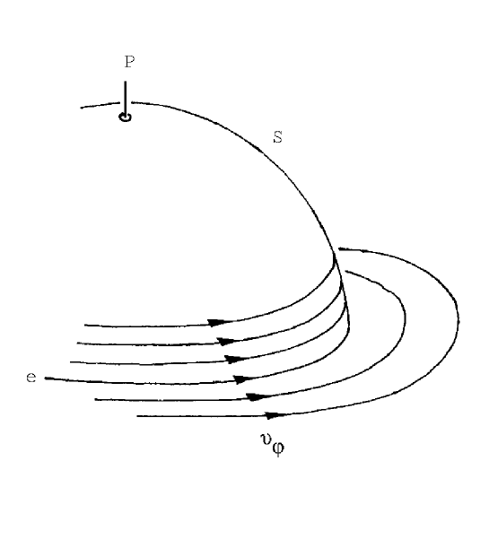
Figure 2: Rotation of the matter in the disk and on the stellar surface in the proposed model; $S$ is the stellar surface, $p$ is the pole, and $e$ is the equator.

In this paper, we take a completely different approach to the problem. The deceleration of rotation is considered simultaneously with the spread of accreted matter (see Figs. 2-4). Discarding popular beliefs, we assume that the deceleration of rotation due to the gripping on (hooking, catching on) the slowly moving dense matter beneath the underlying surface, $S,$ is the principal friction mechanism. This gripping is due to the turbulent viscosity. This problem has much in common with the well-studied (both theoretically and experimentally) problem of the deceleration of a subsonic or supersonic flow above a solid surface (see Subsec. 2.5 for a detailed discussion of the turbulence description accepted in this paper).

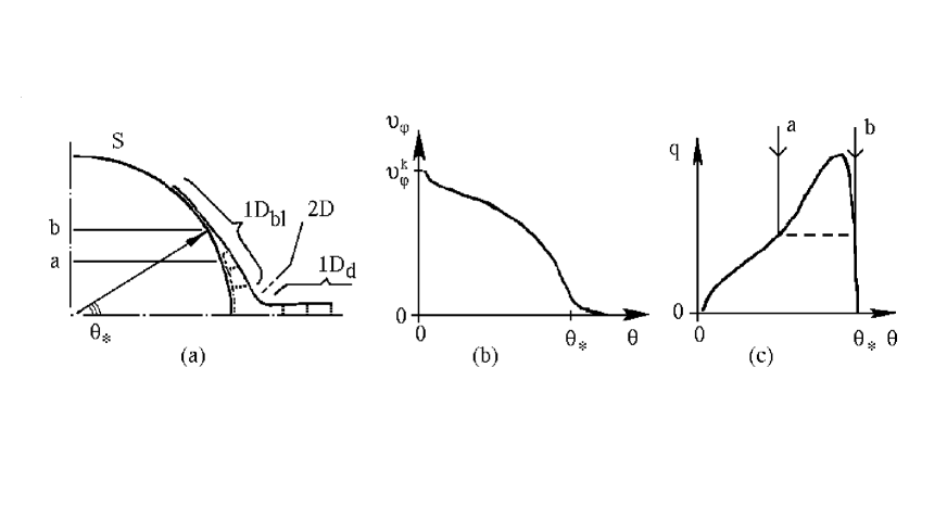
Figure 3: Proposed model: (a) the star is the sphere $S,$ the one-dimensional spread layer is $1D_{bl},$ the two-dimensional transition between the disk and the spread layer is $2D,$ and the one-dimensional disk is $1D_{d};$ (b) the linear rotation velocity $v_{\varphi}$ versus latitude. The rotation is ”localized” in the latitude belt $0<\theta<\theta_{\star}$ – for a nonrotating star, the matter outside this belt is essentially nonrotating; (c) local radiative flux $q$ versus latitude. The arrows $a$ and $b$ ”fence” the ring belt of enhanced brightness. In Fig. 3a, this belt lies between the latitudes $a$ and $b.$

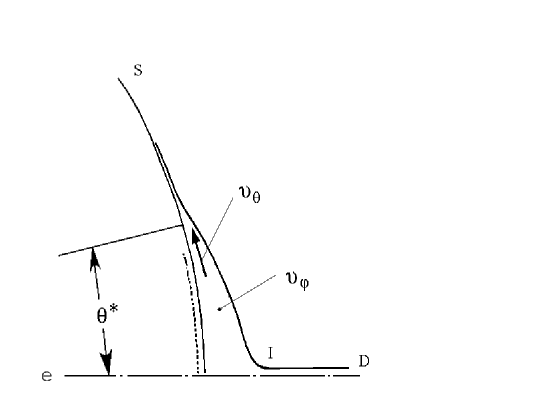
Figure 4: Spread of the rotating plasma from the disk, $D,$ over the neutron-star surface, $S.$ Here, $I$ is the intermediate zone near the disk neck, $0<\theta<\theta^{\star}$ is the hot belt, and $\theta>\theta^{\star}$ is the cold part of the spread layer. The rotation velocity $v_{\varphi}$ (filled circle) is directed along the normal to the plane of the figure. The slowly circulating (in $\varphi$ and $\theta)$ dense underlying layers of matter beneath the spread layer are indicated by the dashes.

Here, we ignore the magnetic field, $H,$ of the neutron star. As we show in Subsec. 4.8, this assumption is valid for $H<2.4\times 10^{9}(L_{SL}/L_{edd})^{0.57}$ gauss, where $L_{SL}$ and $L_{edd}$ are the spread-layer luminosity and the Eddington critical luminosity, respectively. In addition, when deriving the equations of motion of the accreting flow over the stellar surface, we disregard its rotation and general-relativity effects. An appreciable fraction of the X-ray bursters are neutron stars with a rotation frequency $f_{ns}=\omega_{ns}/2\pi$ of the order of 300 Hz see, e.g., a review by Van der Klis 1998). At the same time, the Keplerian rotation frequency $f_{k}=\omega_{k}/2\pi$ at the disk-star boundary in the problem under consideration is about 2000 Hz. Thus, the effects of stellar rotation, which are of the order of the ratio $(f_{ns}/f_{k})^{2},$ are small, and the computations which are performed below also yield an acceptable first approximation to the problem of accretion onto a rotating neutron star.

1.1 Comparison of the Standard and Proposed Approaches

The most important points (I-IV) that pertain to our comparison of the approaches are listed below

(I) Let’s consider the relationship between the radial (inflow to the star, $v_{r}<0)$ and meridional $(v_{\theta})$ velocities. The meridional velocity is commonly ignored $(|v_{r}|\gg v_{\theta}).$ The one-dimensional $(1D)$ approach to the accreting disk also extends to the boundary layer. In any case, $v_{\theta}$ is generally omitted from the equations. The boundary layer turns out to be an extension of the disk in the sense that the $1D$ description of the disk $(1D_{d})$ also applies to the boundary layer. The disk thickness $h$ passes through a minimum near the neck (see Fig. 1a). After the neck, the flow broadens as it approaches the stellar surface and ’digs itself’ into the star.

Meanwhile, a flow with an approximately $1D$ disk, with a $2D$ region of a sharp turn of the flow near the neck, and with an approximately $1D$ (hydraulic) spread of the boundary layer over the neutron-star surface seems more natural (see Figs. 1, 3, 4 and Subsec. 2.1). In this case, $v_{\theta}\gg|v_{r}|$ in the boundary layer. We specify inflow conditions at the interface between the boundary layer and the $2D$ region when calculating the former, because we do not consider here an exact $2D$ problem of the flow in the intermediate zone. In this formulation, it would be more correct to talk not about the boundary layer of the disk but about the spread layer. The dynamics of the latter bears no relation to the disk. Here, the problem of the deceleration and spread of the rapidly rotating matter arises.

(II) We consider the deceleration of rotation and the structure of isolines of rotation velocity $v_{\varphi}.$ In the standard and proposed approaches, we have $v_{\varphi}=v_{\varphi}(r)$ and $v_{\varphi}=v_{\varphi}(\theta)$ in the boundary layer, respectively. The lines of constant $v_{\varphi}$ (isolines) are perpendicular to the equatorial plane in the standard model and perpendicular to the surface $S$ in the proposed model. In both cases, the rotation is Keplerian in the disk at $r>r_{n},$ where $r_{n}$ is the neck radius.

The $v_{\varphi}$ isolines are indicated in Fig. 3a by the dots. They are roughly perpendicular to the surface $S$ inside the boundary layer. The isolines make a sharp turn near $S$ and then run in a dense bundle beside $S$ for a star at rest. This implies that the rotation velocity $v_{\varphi}=\omega r$ abruptly decreases near the interface between the spread layer and the underlying surface. The deceleration near the surface $S$ is discussed in Subsec. 2.5.

(III) In the standard models, the boundary layer and main energy release concentrate near the equator (see Fig. 1). In the proposed model, the width $\theta_{\star}$ of the rotating belt is variable. It increases with increasing accretion rate, $\dot{M}.$ As $\dot{M}\to\dot{M}_{pole},$ the rotation extends to the entire stellar surface: $\theta_{\star}\to 90^{0}.$ Calculations show that the spread-layer luminosity which corresponds to this accretion rate is $L_{pole}\approx 0.9L_{edd,}$ where

$$L_{edd}=4\pi R^{2}q_{0}=1.26\times 10^{38}\frac{M}{M_{\odot}},\;\mbox{erg/s},$$

$$q_{0}=\frac{m_{p}\,g_{0}\,c}{\sigma_{T}}=\Sigma_{T}\,g_{0}\,c=1.00\times 10^{25}\frac{(M/M_{\odot})}{R_{6}^{2}},\;\mbox{erg/s cm}^{2},$$

where $g_{0}=\gamma M/R^{2}=(v^{k}_{\varphi})^{2}/R,$ $v^{k}_{\varphi}$ is the Keplerian velocity at the stellar surface, $\Sigma_{T}=m_{p}/\sigma_{T}=2.5$ g/cm² defines a column of matter with a unit optical depth for Thomson scattering, $m_{p}$ is the proton mass (the plasma is assumed to be hydrogenic), $\sigma_{T}=(8\pi/3)(e^{2}/m_{e}c^{2})^{2}$ is the Thomson scattering cross section, and $R_{6}=R/(10$ km). Below, we talk only about the spread-layer luminosity at the stellar surface normalized to the critical Eddington luminosity. Clearly, the accretion disk makes a comparable contribution to the system’s total luminosity.

(IV) We consider the latitude dependence of the intensity of radiation $q$ from the belt. In the standart approach, the function $q(\theta)$ has a maximum on the equator. In the approach under discussion, $q(\theta)$ turns out to have a minimum at $\theta=0^{0}.$ Moreover, $q(\theta=0)\approx 0.$ The distribution of $q$ (see Fig. 3c) resembles the letter M, if the plot is complemented with the half which is symmetric around the equator.

1.2 Characteristic Features of the Model

The problem of the spread of rapidly rotating accreting matter over a neutron-star surface has several important features.

(I) The centrifugal force which acts on the accreting matter in the vicinity of the equator essentially offsets the gravitation, because the accreting matter in this vicinity has a velocity that is approximately equal to the Keplerian velocity. As one recedes toward the pole, the centrifugal force decreases due to the deceleration of rotation.

(II) In the radiating belt, the radiation pressure works against the difference between the gravitational component and the normal component of the centrifugal force. Because of the rapid rotation, the local Eddington luminosity at which the radiation-pressure force equals the pressing force is appreciably lower than the luminosity $q_{0}$ calculated from the standard formula (1.1).

(III) The dissipation of rotational kinetic energy causes a strong energy release near the lower boundary of the spread layer. As a result, powerful radiation, which diffuses through the spreading plasma and forms the observed spectrum, is produced in this sublayer. The normal component of the gradient in the radiation pressure (or the normal component of the radiation-pressure force) is opposite the direction of the gravitational force. Its direction coincides with the direction of the normal component of the centrifugal force. Within the layer, the normal component of the radiation-pressure gradient (together with the centrifugal force) decreases the free fall acceleration, decreases the density of the matter in the layer, and increases its thickness. An important point is that the increase in the height of the column (in the spread-layer thickness) and the drop in the plasma density cause the efficiency of the turbulent friction of the layer against the stellar surface to decrease. As a result, the deceleration of Keplerian rotation occurs on larger meridional scales than that for a small radiation-pressure force.

(IV) The numerical solution of the equations of radiation hydrodynamics, which is presented below, gives the following picture. The local radiative flux, $q,$ at the equator is much lower than the Eddington critical value (1.1). This is attributable to the action of the centrifugal force and to the fact that the rotation velocity $v_{\varphi}$ near the equator is close to the Keplerian velocity. A ring zone in which the energy release increases due to the decrease in the centrifugal force is formed at a distance from the equator along the meridian. Up to $70\%$ of the layer luminosity is released in two such latitude rings (see Figs. 3a and 3c). In this case, the local flux $q$ never reaches the Eddington limit (1.1), because the finite rotation velocities $v_{\varphi}$ are required for the energy release through friction against the underlying layers, while the allowance for the centrifugal force turns out to be important. The flux $q$ at maximum depends on accretion rate and accounts for $70-97\%$ of the limit (1.1).

(V) The spreading plasma within the bright belt is radiation-dominated $(p_{r}\gg p_{pl}).$ The high saturation of the radiating belt with radiation causes the speed of sound, $c_{s},$ in the layer, which proves to be much larger than the speed of sound in plasma without radiation, to increase significantly. As a result, the flow rotation velocity, $v_{\varphi},$ in the layer is moderately supersonic: $\mathop{\rm Ma}\nolimits_{\varphi}=v_{\varphi}/c_{s}\sim 5.$ The meridional spread is subsonic, which is important in choosing a friction model. If the Mach numbers, $\mathop{\rm Ma}\nolimits_{\varphi},$ were calculated from the plasma speed of sound alone, then the flux would be hypersonic with $\mathop{\rm Ma}\nolimits_{\varphi}\sim 100;$ moreover, the flux in $v_{\theta}$ would be transonic.

(VI) At $\theta>\theta_{\star},$ the velocity, $v_{\varphi},$ drops virtually to zero, and the layer contracts to a thin, cold weakly radiating film (’dark’ layer), which slowly moves toward the poles. Having lost the excess (relative to the star) angular velocity in the radiating belt, the matter becomes cold and dense. The intensity of the radiation from its surface decreases by several orders of magnitude. It moves relative to the star with a velocity that is considerably lower than the speed of sound. Of course, this matter is not accumulated near the poles. There is a slow flow in which it spreads under the hot layers over the entire stellar surface. This matter forms the surface against which the radiation-dominated layer rubs.

(VII) If the local radiative flux were the limiting Eddington flux (1.1), the width of the radiating belt (let us denote this width by $\theta^{\star}_{0}$ to distinguish it from $\theta_{\star})$ could be estimated from the energy balance

$$(1/2)\,\dot{M}\,(v_{\varphi}^{k})^{2}=q_{0}\,4\pi R^{2}\,\sin\theta^{\star}_{0},\;\;\;\;\;\theta_{0}^{\star}=\arcsin(L_{SL}/L_{edd}),$$

where $L_{SL}$ is the spread-layer luminosity. As will be seen from the analysis in the main body of this study, $(1.1)^{\prime}$ underestimates appreciably $\theta_{\star}.$ This is attributable to the action of the radial component of the centrifugal acceleration. As follows from the calculations which are given below, the approximate balance is

$$\dot{M}\,\frac{(v_{\varphi}^{k})^{2}}{4}=2\pi R^{2}\,\int_{0}^{\theta_{\star}}\,q_{eff}(\theta)\;d\sin\theta,$$

$$q_{eff}(\theta)=\Sigma_{T}\,g_{eff}(\theta)\,c,\;\;\;g_{eff}(\theta)=g_{0}\,G_{eff}(\theta),\;\;\;G_{eff}=1-U^{2}-W^{2}\approx 1-W^{2},$$

where $U=v_{\theta}/v_{\varphi}^{k},$ $W=v_{\varphi}/v_{\varphi}^{k},$ $v_{\varphi}^{k}$ is the Keplerian velocity. In $(1.2)^{\prime},$ we assumed that the centrifugal force is almost completely determined by the rotation velocity, $v_{\varphi},$ because the centrifugal force related to the spread velocity is small: $v_{\theta}^{2}/R\ll g_{0}.$ The latitude dependence of rotation velocity $v_{\varphi}(\theta)$ is required to calculate $\theta_{\star}$ using (1.2). The approximate validity of relations (1.2) and $(1.2)^{\prime}$ is attributable to the fact that the Eddington radiative flux $q_{r}$ in the radiating belt offsets the difference $g_{eff}$ between the weight and the radial component of the centrifugal force with a high precision [see below Subsec. 1.3 (I)]. The appearance of rings of enhanced luminosity follows precisely from this. Indeed, it follows from $(1.2)^{\prime}$ that $q(\theta)$ increases with $\theta,$ because $v_{\varphi}(\theta)$ decreases with latitude.

(VIII) We carried out this study in an effort to explain the observed spectra of bursters in a wide range of their luminosities. Several variable sources that are X-ray bursters exhibit variations in the X-ray luminosity by hundreds of times (see Campana et al. 1998a, 1998b, Gilfanov et al. 1998). The theory, which we construct here, claims to describe some of the spectral features in the light curve of a neutron star as the luminosity changes by two orders of magnitude.

(IX) The atmosphere under consideration is characterized by the delicate balance of three forces: gravitation, centrifugal force, and radiation-pressure force. Under these conditions (just as in the atmospheres of massive hot stars), a strong wind which flows away from the zone of enhanced brightness is inevitably formed. As a first approximation, we assume below that this wind affects only slightly the transport characteristics of the spread layer and its optical depth.

(X) It follows from the qualitative estimates and the detailed calculations which are presented below (see Subsecs. 4.3 and 4.5) that the derived solutions in the radiating belt lie near the limit of validity of the shallow-water approximation. The ratios of the effective layer thickness, $h_{eff}=[\,|\,d\ln\rho/dr\,|\,]^{-1},$ in this region (the derivative is calculated near the base of the spread layer) to the stellar radius, $R,$ are typically $\sim 0.1.$

Figure 5: Profiles 1, 2, 3 and 4 of the spread-layer (S.L.) effective thickness $h_{eff}(\theta)$ for various accretion rates $\dot{M}.$ The relative luminosities, $L_{SL}/L_{edd},$ that correspond to labels 1, 2, 3 and 4 are 0.01, 0.04, 0.2 and 0.8, respectively. The stellar mass and radius are $1.4M_{\odot}$ and 12 km. (a) Linear scales, the shape of the radiating belt is seen; (b) logarithmic scales, the dark layer and the spread layer are seen better than in the upper panel (especially at small $\dot{M};$ the scale $R\theta$ covers the entire distance from the equator to the pole).

Nevertheless, the hydraulic approximation (Schlichting 1965; Chugaev 1982) describes satisfactorily the experimental situation at the values of $h_{eff}/R.$ The geometrical characteristics of the spread layer are shown in Fig. 5. The spread layer is divided into two distinctly different parts at $\theta_{\star}:$ the radiating belt (r.b.) and the dark layer (d.l.). Their thicknesses, $h_{rb}$ and $h_{dl},$ differ markedly. The thickness $h_{dl}$ is of the order of the scale height in a gravity field with $g_{0}=\gamma M/R^{2}.$ The slope $\tan\beta$ is $dh_{eff}/Rd\theta.$ This slope changes only slightly inside the radiating belt (see Fig. 5a). The angle $\beta$ is very small in the dark layer. The angle $\beta$ in the radiating belt increases as the accretion rate, $\dot{M},$ decreases. Therefore flows with low $\dot{M}$ are described worse by the $1D$ approximation. In Figs. 5a and 5b, profiles 1-4 refer to the different values of $\dot{M}.$ Profiles 1-4 from Fig. 5a are repeated in Fig. 5b on a logarithmic scale. This is necessary because the dark-layer thickness, $h_{dl},$ is so small that it cannot be compared with the radiating-belt thickness $h_{rb}$ on a linear scale. In addition, the flow separation into two characteristic regions is more clearly seen in Fig. 5b. The latitude $\theta_{\star}$ corresponds to the thin transition zone of a rapid change in thickness. In turn, the linear coordinates in Fig. 5a are required to show the shape of the radiating belt.

(XI) The flows in the disk and in the spread layer are closely related. The accreting flow is furnished through the disk, while irradiation of the disk from the stellar surface affects its characteristics. This issue is analyzed in Subsec. 2.1, where the disk thickness in the zone of its contact with the spread layer is estimated.

(XII) In a radiation-dominated layer, the hydrodynamic meridional transfer of radiative enthalpy toward the poles plays a major role. This enthalpy per unit mass is of the order of the gravitational energy $\gamma M/R.$

1.3 Main Results

We derive the system of equations of radiation hydrodynamics that describes the deceleration of rotation of the accreting matter and its meridional spread. The derivation is based on the assumption that Thomson scattering contributes mainly to the opacity and that the energy release concentrates in a relatively thin sublayer at the base of the spread flow. The derived equations differ markedly from the standard shallow-water equations. A qualitative analysis of the derived system of equations and their solutions (Sec. 3) allows us, first, to develop a procedure for the effective numerical integration of the equations and, second, to make a clear interpretation of the calculations. We carried out a numerical analysis of the system. The problems of the numerical analysis, without which an independent verification of the data would be impossible, are outlined in Secs. 3 and 4. It is important to set out the procedure for the solution, because if this procedure is clear the results can be reproduced. We thus would like to draw the reader’s attention to the following subsections: (I) smallness of the coefficients, rigidity of the system, steep and gentle segments (Subsec. 3.5); (II) multiplicity of the solutions, selection criteria (Subsecs. 3.6 and 4.1-4.4); (III) circulation of the cooled accreting matter which lost the rotational velocity component, its spread and settling (Subsecs. 4.2-4.4); and (IV) modification of the solutions as the friction coefficient and the accretion rate are varied (Subsecs. 4.5 and 4.7).

Below, we dwell on the most important results.

(I) Rings of enhanced brightness. Typical latitude profiles of the flux $q$ are shown in Figs. 6-8. The radiating belt broadens as the accretion rate increases. The latitude $\theta_{max}$ at which the bright rings lie increases with increasing $\dot{M}$ and $L_{SL}/L_{edd}.$ The bright rings are not narrow; their width is $\Delta\theta\simeq\theta_{\star}.$ At a high accretion rate $\dot{M}\simeq\dot{M}_{pole}$ [see Subsec. 1.1 (III)], the entire stellar surface, except the small equatorial and polar zones, emits almost uniformly. In this case, the bright ring spreads out. Profile 4 in Fig. 7 refers to this situation.

Figure 6: Local radiative flux $q(\theta)$ (solid lines) and effective free fall acceleration (including the centrifugal acceleration) $g_{eff}(\theta)$ (dashed lines) versus latitude. An important point is that $q/q_{0}\approx g_{eff}/g_{0}$ in the radiating belt [see (1.2) and (1.2)’]. Labels 1 and 3 refer to $L_{SL}/L_{edd}=0.01$ and $0.2,$ respectively.

Figure 7: Changes in the profiles of the local radiative flux $q$ (solid lines) with $\dot{M}.$ The radiating belt broadens with increasing $\dot{M}.$ The boundary $\theta_{\star}$ lies at the right edge of the belt in the zone of an abrupt decrease in $q(\theta).$ The $g_{eff}/g_{0}$ profile at $L_{SL}/L_{edd}=0.8$ is indicated by the dashed line. The scale $R\theta$ terminates at the pole. Labels 2, 3, and 4 refer to $L_{SL}/L_{edd}=0.04,0.2,$ and 0.8, respectively.

Figure 8: $q(\theta)$ profiles in a wide range of $\dot{M}.$ Labels 1, 2, 3, and 4 refer to $L_{SL}/L_{edd}=0.01,0.04,0.2,$ and $0.8,$ respectively.

The function $q(\theta),$ which gives the radiative flux, has the maximum at $\theta_{max}$ with which the ring of enhanced brightness is associated. This ring is marked by arrows $a$ and $b$ in Fig. 3c. The ring bounded by latitudes $a$ and $b$ which correspond to these arrows is shown in Fig. 3a. To the right of $\theta_{max},$ the rotation velocity $v_{\varphi}$ vanishes (see Figs. 3b and 3c). For this reason, $q(\theta)$ rapidly decreases to the right of $\theta_{max}.$ The increase in $q(\theta)$ to the left of $\theta_{max}$ (see Fig. 3c) with increasing $\theta$ is caused by the decrease in $v_{\varphi}$ (see Fig. 3b). Indeed, the decrease in $v^{2}_{\varphi}$ leads to an increase in the acceleration $g_{eff}\approx g_{0}\,(1-W^{2}),$ where $W=v_{\varphi}/v_{\varphi}^{k},$ and, consequently, to an increase in $q,$ $\;q\propto g_{eff}$ [see formulas (1.2) and $(1.2)^{\prime}].$

Figure 9: Profiles of the meridional velocity $v_{\theta}$ and of the spread-layer surface density $\Sigma_{S}$ for $L_{SL}/L_{edd}=0.2.$ At $\theta_{\star},$ the flow abruptly slows down, and its density increases. In the upper corner, the Keplerian velocity $v_{\varphi}^{k}$ is shown for $M=1.4M_{\odot}$ and $R=12$ km.

(II) Surface density, optical depth, and spectral hardness. In the steady-state case in the absence of sources and sinks of matter in the spread layer, the flux of mass is conserved when spread along the meridian. We ignore the settling of matter to the bottom within this layer (Subsecs. 4.3 and 4.4). The meridional velocity is thus $v_{\theta}\propto 1/\Sigma_{S},$ where $\Sigma_{S}=\int\rho dr$ is the surface density, the integral is taken over the spread-layer thickness. Accordingly, $\Sigma_{S}$ reaches a minimum at the maximum of $v_{\theta}.$ These profiles are illustrated in Fig. 9. The spread layer consists of the radiating belt and the dark layer which border at $\theta_{\star}.$ The maximum of $v_{\theta}$ and the minimum of $\Sigma_{S}$ lie near the edge of the radiating belt. In the dark layer, $\Sigma_{S}$ abruptly increases, while $v_{\theta}$ abruptly decreases. This is clearly seen in Figs. 9 and 10. The dark layer terminates at the sonic point. This important problem is analyzed in Subsecs. 4.1-4.4.

Figure 10 shows how the spread-layer surface density $\Sigma_{S}$ depends on accretion rate. The spread-layer optical depth $\tau_{T}=\Sigma_{S}/\Sigma_{T}$ for Thomson scattering rapidly decreases with decreasing $\dot{M}.$ At $L_{SL}/L_{edd}\sim 10^{-2},$ we have $\tau_{T}\sim 3.$ No blackbody radiation can be produced in the medium at such a small optical depth; the protons and electrons have temperatures much higher than 1 keV. The low-frequency photons emitted by the dense underlying layers are comptonized by hot electrons of the spread layer and form the experimentally observed hard power-law tails in the spectra (Barret et al.1992, Campana et al. 1998a, 1998b, Gilfanov et al. 1998). In turn, some of the hard photons penetrate deep into the underlying layer and heat it up [see Sunyaev and Titarchuk (1980) for a discussion of this problem].

Figure 10: Shape of the $\Sigma_{S}(\theta)$ profile at different spread-layer luminosities. At a fixed $\dot{M},$ the surface density rises with increasing $\theta$ at $\theta_{\star},$ after which an optically thick weakly radiating layer begins. Labels 1, 2, 3, and 4 refer to $L_{SL}/L_{edd}=0.01,0.04,0.2,$ and $0.8,$ respectively.

At a high spread-layer luminosity $L_{SL}>0.1L_{edd},$ we have a different picture. In this case, the spectrum is much softer and exhibits no pronounced hard tail. The optical depth for Thomson scattering is great $(\tau_{T}\sim 1000).$ The layer optical depth for effective absorption $\sqrt{\tau_{T}\;\tau_{ff}(\nu,T_{e})}$ (Shakura 1972; Felten and Rees 1972; Shakura and Sunyaev 1973; Illarionov and Sunyaev 1972) turns out to be also large. Deep in the layer, the most important physical process is saturated comptonization. The parameter $y=(T_{e}/m_{e}c^{2})\,\tau_{T}^{2},$ which characterizes comptonization in a layer with an optical depth $\tau_{T},$ is large even at $\tau_{T}>\sqrt{m_{e}c^{2}/T_{e}}\sim 20.$ At $T_{e}\sim T\sim\tau_{T}^{1/4}$ (see Subsec. 2.2) and $\tau_{T}\sim 10^{3},$ we have $y\sim(T_{S}/m_{e}\,c^{2})\,\tau_{T}^{9/4}\sim 10^{5}$ deep in the layer. The dimensionless frequency, near which the rate of photon absorption due to the free-free processes equals the rate of photon removal upward along the frequency axis via comptonization, is $x_{0}=h\nu_{0}/T_{e}=3\times 10^{5}\,n_{e}^{1/2}/T_{e}^{9/4}.$ This frequency, deep in the layer, is high. Here, the electron density is in cm${}^{-3},$ and the electron temperature is in Kelvins. As can be seen from the plots in Illarionov and Sunyaev (1975), comptonization produces the Wien spectrum deep in the layer at $y>10,$ while at $y>10^{5}$ the spectrum is similar to a blackbody due to the comptonization of low-frequency photons. Consequently, the combined effect of bremsstrahlung and comptonization produces a blackbody spectrum deep in the layer. The emission from the dense underlying layers is yet another source of soft photons for comptonization. Nevertheless, the emergent spectrum differs markedly from a blackbody spectrum, because at each frequency we see a portion of the spectrum that is produced at its own depth [see Illarionov and Sunyaev (1972) for a discussion of this problem].

Integrated spectrum of the spread layer. The spread-layer spectrum is given by the integral of the emergent spectra at each point of the layer over its surface. Here, it is important that the spectrum and the local radiative flux depend on latitude. The integrated spectrum is not presented for the following two reasons.

(a) A considerable fraction of the spread-layer radiation falls on the disk surface (see Fig. 2). This fraction is partially reflected from the disk and partially reprocessed by it into softer radiation. The intensity of the disk-reprocessed radiation depends on the binary’s inclination (see Lapidus and Sunyaev 1985). Allowance for these effects requires a special study.

(b) Because of the shielding by the disk, the observer cannot see the lower half of the neutron star. Part of its surface is located in the shadow region and does not contribute to the direct rays viewed by the observer (here, we disregard the general-relativity effects). In Fig. 11, the flux of ”direct” photons from the stellar surface is plotted against the cosine of the binary’s inclination angle, $i,$ which is measured from the star’s polar axis (see Figs. 1-4). In these calculations, we assumed the indicatrix of emission per unit area to be $\varphi(\mu)=1+2.06\,\mu\;(\mu=\cos i);$ this is the first approximation for the angular dependence of the intensity of the emergent radiation from a scattering atmosphere (Sobolev 1949; Chandrasekhar 1960). In the calculations, we took into account the profiles $q(\theta)$ (see Figs. 6-8).

Figure 11: Functions $I(\mu)/I(0)$ $[I$(erg s^-1 steradian${}^{-1},$ $\;\mu=\cos i]$ which give the intensity of the radiation from the visible neutron-star surface. The binary’s inclination, $i,$ is measured from the polar axis. Labels 1, 2, 3, and 4 refer to $L_{SL}/L_{edd}=0.01,0.04,0.2,$ and $0.8,$ respectively. The functions are normalized to the intensity of the radiation from the equator $I(0).$

Clearly, the presence of a ”shadow” and the reflection by the disk must lead to an appreciable polarization of the emission from an accreting neutron star. At low luminosities, at which the radiating belt is bound by the equatorial zone, the flux toward an observer in the equatorial plane $(\mu=0)$ exceeds the flux toward the polar axis $(\mu=1).$ Curves 1-3 in Fig. 11 correspond to these luminosities. At high luminosities, the emission extends to the entire stellar surface (curve 4 in Fig. 7). In this case, the flux toward the polar axis is greater than the flux toward the equatorial plane (curve 4 in Fig. 11). Indeed, the ratio $I(1)/I(0)=2$ for a uniform emission of the stellar surface, because the disk occults the lower stellar hemisphere.

(III) Deceleration efficiency. The meridional distributions of rotation velocity $v_{\varphi}$ are shown in Fig. 12. We performed the calculations for $\delta=10^{-2},$ where $\delta=1-W_{0}=(v^{k}_{\varphi}-v^{0}_{\varphi})/v^{k}_{\varphi},$ where $v^{0}_{\varphi}$ is the initial rotation velocity in the spread layer when passing from the disk to the layer, and $v^{k}_{\varphi}$ is the Keplerian velocity (see Subsecs. 3.4 and 4.6). Similar results are also obtained for different values of $\delta\ll 1.$ As $\dot{M}$ increases, the deceleration of rotation requires an increasingly large area of contact between the radiating belt and the stellar surface. The boundary of this belt is $\theta_{\star}.$

Figure 12: Meridional profile of the rotation velocity. The radiating belt is simultaneously the rotating belt (cf. Figs. 6-8). Labels 1, 2, 3, and 4 refer to $L_{SL}/L_{edd}=0.01,0.04,0.2,$ and $0.8,$ respectively.

An interesting characteristic of the deceleration efficiency is the number of rotations a test particle makes around the star before it looses its rotation velocity and reaches the latitude $\theta_{\star}.$

Table. Dependencies of $\theta_{\star},$ $N_{rot}$ and $q/Q^{+}$ on $L_{SL}/L_{edd}.$

$L_{SL}/L_{edd}$	0.01	0.04	0.2	0.8
$R\theta_{\star},$ km	0.43	1.36	4.5	16.4
$N_{rot}$	0.3	1.1	5.4	36
$(q/Q^{+})_{max}$	1.01	1.05	1.3	3.8

The table shows how the width of the belt $\theta_{\star}$ and the number of rotations,

$$N_{rot}=\Delta\varphi/2\pi,\;\;\;\;\;\Delta\varphi=\int_{\theta_{0}}^{\pi/2}\,\omega\,dt\approx\int_{0}^{\theta_{0}}\frac{v_{\varphi}}{v_{\theta}}\;\frac{d\theta}{\cos\theta},$$

of its rotating plasma depend on the spread-layer relative luminosity $L_{SL}/L_{edd.}$

As we see from the table, at a low spread-layer luminosity $(0.01L_{edd}),$ a test particle does not make even one rotation around the star, rising by 430 m along the meridian and covering 23 km in latitude. Note that the meridional boundary-layer extent (see Fig. 1) $R\theta_{bl}=R\sqrt{2T_{bl}/m_{p}}/v_{\varphi}^{k}$ is a mere 70 m in the standard approach (at $T_{bl}=3$ keV). At a high luminosity, the deceleration efficiency is much lower: at $L_{SL}=0.8L_{edd},$ test particles make 36 rotations around the star before they slow down and reach $\theta_{\star}.$

(IV) Advection of radiative energy. The spreading matter in an optically thick layer transports radiative energy along the meridian from the equatorial region into the region of the bright rings. The energy transfer is described by the energy equation (see Subsecs. 2.7 and 3.2). Our calculations (see Fig. 13) show that the energy flux $q$ emitted per unit area of the spread layer in the equatorial region is much smaller than the local energy release through the turbulent friction in a column $Q^{+}=\int\,\dot{\epsilon}_{t}\,dy,$ where the integral is taken over the spread-layer thickness [Subsec. 2.5, (2.17)]. On the other hand, the flux $q$ at higher latitudes for larger luminosities exceeds appreciably $Q^{+}$ [see the table, which gives the dependence of maximum $(q/Q^{+})_{\max}$ in the spread layer on $L_{SL}/L_{edd}].$ This is only to be expected, because the spread-layer optical depth for Thomson scattering is large at high luminosities. As a result, the characteristic diffusion time $t_{d}$ of the photons from the base of the hot layer turns out to be of the order of the time of hydrodynamic motion $t_{h}$ through the radiating belt, where $t_{d}\sim(h/c)\,\tau_{T}$ and $t_{h}\sim R\theta_{\star}/v_{\theta}.$ The advection of radiative energy favors the formation of bright latitude rings at the stellar surface.

Figure 13: Spread dynamics is determined in many ways by the hydrodynamic transfer of radiative energy. The ratio of the energy flux, $q,$ emitted per unit area of the radiating layer to the frictional energy release $Q^{+}$ per unit area of the contact surface between the spread layer and the star. The energy is transferred from zone A into zone B through meridional advection. This calculation is for $L_{SL}/L_{edd}=0.2.$

1.4 Problems That Require Further Studies

(I) Possible Instability of the Spread Layer. The energy-producing sublayer props up the spread flow from below, and the radiation pressure dominates. This may be the cause of convective instability with floating ’photon bubbles’. Clearly, this requires that the spread layer be optically thick. The fluctuations which are produced by the bubbles may be responsible for the observed low-frequency noise and even for quasi-periodic oscillations in accreting neutron stars. Although, on the other hand, the rotation velocity, $v_{\varphi},$ inside the spread layer outside the energy-producing sublayer, along with the normal component of the centrifugal force, slightly increases with height. In addition, the tail of the volume density of dissipative energy production $\dot{\epsilon}_{t}$ erg s^-1 cm^-3 extends from the energy-producing sublayer into the spread layer. As a result, the flux $q$ and, hence, the Eddington force slightly increase with distance from the surface. These two effects play a stabilizing role with respect to the convective instability. The instability is also stabilized by turbulent viscosity and turbulent diffusion, which are attributable to the presence of a wall (the stellar surface from below) and of shear turbulence. This turbulence causes, first, the mixing of density fluctuations (diffusive mixing of photon bubbles) and, second, the momentum exchange between the bubbles and the ambient medium (viscous deceleration). The problem of the vertical stability of hydrostatic quasi-equilibrium, indubitably, requires further study.

(II) Gap between last stable orbit and surface. Here, we do not consider the case where the stellar radius $R$ is smaller than the radius of the marginally stable Keplerian orbit $R_{c}=3R_{g}.$ In this case, part of the gravitational energy is released in the zone of contact between the disk and the star due to an appreciable radial velocity (it increases with the increasing $R_{c}-R)$ of the accreting matter on the stellar surface. The energy release at the equator causes the layer to swell in this zone because of the radiation pressure, and the $1D$ approximations appear to become inapplicable.

(III) Rapid rotation. The case of rapid rotation of a star, where its angular velocity, $\omega_{S},$ accounts for an appreciable fraction of the Keplerian angular velocity, $\omega_{k},$ requires a special analysis.

1.5 Structure of the Paper

Here, we derive and numerically solve the system of equations of motion of the matter over a neutron-star surface in the $1D$ approximation. The vertical (along $r)$ and horizontal (along the meridian $\theta)$ scales are separated in this approximation. The gradients in $r$ are assumed to be large compared to the gradients in the polar angle $\theta.$ For this reason, the vertical profile is constructed from the conditions of hydrostatic quasi-equilibrium. The profile is given by simple analytic expressions. The averaging of the quantities over the vertical structure with which the derivation begins allows us to obtain a system of equations for these quantities that contains only gradients in $\theta.$ These are the equations of radiation-dominated shallow water that describe the dynamics of the high-velocity layer in which the newly accreted matter flows over the surface of the slowly moving high-density underlying layers (Sec. 2). This completes the part of the paper in which we formulate the problem. The part in which we present the results is devoted to the steady-state solutions of our model. In this part, we describe the physics of adaptation: effects of the friction model, Eddington swelling of the boundary layer, regulation of the deceleration by the swelling, etc. (Secs. 3 and 4). We study the mathematical properties of radiation-dominated shallow water: the structure of the solutions, the limiting set of steady-state solutions, its one-parameter structure, the critical solution, etc. (Sec. 3). We analyze the dependences of the boundary-layer characteristics on $\dot{M}$ and on model parameters (Secs. 3 and 4). Note that it follows from the solutions that the bulk of the radiating belt is roughly in hydrostatic equilibrium along the meridian, as was previously suggested by Shakura and Sunyaev (1988). In this case, the ”pressing” force to the equator is the tangential component of the centrifugal force, which counteracts the meridional component of the pressure gradient.

The interaction of the spreading flow with the underlying matter is described in Subsec. 2.1. Here, we also estimate the effects of disk heating by the spread-layer radiation and determine the minimum possible disk thickness near the neck. The neck forms a kind of base of the disk at the location of its interaction with the spread layer. In Subsec. 2.2, we determine the structure of a radiation-dominated atmosphere in which the scattering by free electrons is a major contributor to the opacity. The force and energy characteristics of this atmosphere which are required to calculate its energy and transport properties are derived in Subsec. 2.3. A simple formula for radiative losses in the spread layer is written out in Subsec. 2.4. Subsec. 2.5 deals with the friction model. In Subsecs. 2.6 and 2.7, we derive the equations of ”radiation” shallow water. Transformations of this system of equations are made in Subsecs. 3.1-3.3. In Subsecs. 3.4 and 3.5, we study the phase space of the system and introduce an important surface – the ”levitation” surface. The dependence of the spread velocity on the Mach number is analyzed in Subsec. 3.6. The solutions of the derived system of equations are analytically and numerically analyzed in Subsecs. 4.1 and 4.2. Subsec. 4.3 investigates the critical regime in which the spread velocity reaches the speed of sound for the spread of matter at the edge of the radiating belt. The dynamics of the matter spread outside the radiating belt is analyzed in Subsec. 4.4. The effect of friction on the results is considered in Subsec. 4.5. Such an analysis is necessitated by the fact that, first, the friction coefficient is determined only approximately and, second, this coefficient decreases by a factor of 1.5 to 2 in the supersonic regime (see Subsec. 2.5). We construct the dependence $q(\theta)$ in Subsec. 4.6 and study how the spread flow is modified as the accretion rate $\dot{M}$ is varied in Subsec. 4.7. At large $\dot{M},$ the ”squeezing” of the flow due to the convergence of meridians to the pole becomes important. In addition, the spread flow in the radiating belt is strongly subsonic at high $\dot{M}$ and transonic at low $\dot{M}.$ In Subsec. 4.8, we estimate the limiting magnetic field strength that can still be ignored when the deceleration and spread are studied. The results are summarized in the conclusion.

2 HYDRAULIC APPROXIMATION

2.1 Spread Scheme

The spread flow is illustrated in Fig. 4. Here, $e$ is the equatorial plane, $D$ is the disk, $I$ is the transition region between the disk and the boundary layer (the region of $2D$ flow), and $S$ is the stellar surface. Let $h(\theta)$ be the boundary-layer thickness. For the $1D$ approximation to be valid, it is necessary that

$$h\ll R,\;\;\;\;\;\;\;\;\;|dh/dl|\ll 1,$$

where $l=R\theta$ is the arc length along the meridian. Note, incidentally, that it follows from the calculations (see below) that the angle $\arctan|dh/dl|$ is constant in order of magnitude at $0<\theta<\theta_{\star}.$

The latitudinally and meridionally moving spread layer draws (grips) the thin underlying layers into motion via turbulent friction. The underlying layer is indicated by the dashed line in Fig. 4. The $v_{\varphi}$ distribution inside the boundary layer is roughly uniform in height (see Subsec. 2.5 for a discussion). Almost all of the drop in $v_{\varphi}$ takes place near the surface, $S,$ which is the bottom of the boundary-layer, $r=r_{S}$ or $y=y_{S}.$ The main turbulent energy release occurs near the bottom. Since the problem is a steady-state problem, the temperature $T$ is constant at $y<y_{S}$ (these layers were heated earlier, and the energy release in them is small), while the vertical radiative flux $q$ is approximately constant above $y_{S}$ and equal to zero below. Because of the abrupt change in $q$ at the surface $S,$ the plasma parameters also change when this surface is crossed. The underlying-layer density $\rho_{2}$ exceeds the boundary-layer density in the hot subregion $0<\theta<\theta_{\star}.$ In the region $\theta>\theta_{\star},$ the density of the underlying layers rapidly increases with depth, because they are isothermal. For this reason, the velocity in the underlying layers rapidly decreases with depth.

Disk heating by spread-layer radiation. Let us find out how the disk thickness near a neutron-star surface will change under spread-layer radiation. The angular rotation velocity $\omega$ of the accreting matter is known to reach a maximum in the transition zone between the disk and the spread layer (Shakura and Sunyaev 1973). Accordingly, $d\omega(r=r_{n})/dr=0.$ This point in the flow is called the neck (see Figs. 1, 3, and 4). The dissipative production of thermal energy vanishes at $r_{n},$ because the derivative of $\omega(r)$ at this point changes sign and because the heat release, which is proportional to $(d\omega/dr)^{2},$ is small in the neck zone. The surface density of viscous energy release in the disk (in Newton’s approximation) behaves as $Q^{+}=$ $(3\gamma M\dot{M}/4\pi r^{3})(1-\sqrt{R/r}).$ At $r\gg R,$ the energy release $Q^{+}$ is a factor of 3 greater than the local gravitational energy release $\gamma M\dot{M}/4\pi r^{3},$ which is attributable to the transfer of mechanical energy by viscous forces over the disk from regions with smaller $r$ to regions with larger $r.$ At the same time, $Q^{+}\to 0$ as $r\to R.$ Therefore, the disk half-thickness, $h=$ $(3/8\pi)(\sigma_{T}\,\dot{M}/m_{p}\,c)(1-\sqrt{R/r}),$ also decreases as one approaches the neck (Shakura and Sunyaev 1973). This consideration ignores disk heating by the spread-layer radiation and the pressure of external radiative flux. Let us estimate how the heating by external radiation affects the disk half-thickness near the neck. Let $T_{s},$ $T_{c},$ and $T_{r}$ be the disk-surface temperature, the temperature in the disk equatorial plane, and the external-radiation temperature, respectively. Since the flux from the spread layer accounts for a fraction of the Eddington flux, its temperature is $T_{r}=1-1.5$ keV. The disk albedo is assumed to be 0.3-0.5. Consequently, the disk surface near the neck will be heated to temperatures of the order of 1 keV. Clearly, the surface temperature under quasi-steady-state conditions (the radial velocity of the matter near the neck is low) is less than or equal to $T_{c}.$ Using a hydrostatic estimate of the half-thickness, $h=Rc_{s}/v_{\varphi}^{k},$ and assuming that $c_{s}\sim\sqrt{T_{c}/m_{p}},$ we obtain $h=30R_{6}^{3/2}\,\sqrt{T_{c}}/\sqrt{M/M_{\odot}}$ m, where $T_{c}$ is in keV, and $R_{6}=R/(10$ km). It thus follows that the disk angular half-thickness, $\theta_{0},$ is finite. The conclusion about the finite but small disk half-thickness near the neck is crucial for the validity of our approach to the problem of accretion onto a neutron star.

Here, we do not consider the advection solution for the flow in the disk (Narayan and Yi 1995) for two reasons. First, the neutron star has a solid surface, and it is, therefore, difficult to imagine accretion without energy release on the surface. Second, the flux from the spread layer is so large that it will cool the plasma flow at a distance of several tens of neutron-star radii through comptonization. As a result, an accretion pattern with a relatively thin (geometrically) accretion disk is most likely realized near the star.

2.2 Structure of the Spread Layer (Atmosphere)

We make the following assumptions:

(I) The energy is mainly released in a thin sublayer near the boundary between the spreading and underlying layers.

(II) Thomson scattering makes a major contribution to the opacity.

(III) We define the free fall acceleration $g_{eff}$ within the spreading layer with allowance for the contribution of the centrifugal acceleration as the difference $g_{eff}=\gamma M/R^{2}-v_{\varphi}^{2}/R-v_{\theta}^{2}/R$ [see (1.1) and (1.1)’]. For completeness, we added the centrifugal acceleration due to the meridional motion. It is small compared to the acceleration $\gamma M/R^{2}.$ The rotation velocity, $v_{\varphi},$ is assumed to be constant within the atmosphere (if $\theta$ is fixed).

Under these assumptions, the atmospheric structure is described by the system of equations

$$p=g_{eff}\;\Sigma,$$

$$q=\frac{c\,\Sigma_{T}}{3}\;\frac{d\epsilon}{d\Sigma},$$

$$p=2\;\frac{\rho\,T}{m_{p}}+\frac{\epsilon}{3},$$

$$\epsilon=a\;T^{4}.$$

The system of equations of hydrostatics (2.2), radiative heat conduction (2.3), thermodynamic state (2.4), and Stefan-Boltzmann’s law (2.5) relates the unknown functions $p,\epsilon,\rho,$ and $T$ of the vertical column density $\Sigma,$ which is a Lagrangian coordinate $(d\Sigma/dy=\rho).$ The $y$ and $\Sigma$ axes are directed downward. Accordingly, the pressure in (2.2) increases with $\Sigma.$ The $q$ is the absolute flux. We assume that the layer borders vacuum $(p=0)$ at $y=0,\Sigma=0.$ The boundary-layer bottom $y=y_{S}=h,$ $\;\Sigma=\Sigma_{S}$ is the surface $S$ (see Fig. 4). The system of equations (2.2)-(2.5) is written for an arbitrary fixed latitude $\theta.$ Due to the approximate assumption of constant $v_{\varphi}(\theta)$ in the boundary layer $0<y<h,$ the acceleration $g_{eff}$ in (2.2) is constant as $\Sigma$ increases deep into the layer.

Eq. (2.3) holds for radiative transfer in an optically thick plasma with $\Sigma_{S}\gg\Sigma_{T}$ with dominating Thomson scattering. We assume that the turbulent dissipation is localized near the surface $S.$ It thus follows that the heat flux $q$ in the spread layer $0<y<h,$ which is transferred via radiative heat conductance, is approximately constant. The total pressure consists of the plasma and radiation pressures.

The system of equations (2.2)-(2.5) can be easily solved. The solution that satisfies the boundary condition

$$p(0)=0,\;\;\;\epsilon(0)=0,\;\;\;\rho(0)=0,\;\;\;T(0)=0,$$

is

$$p=g_{eff}\Sigma,\;\;\;\epsilon=\frac{3q}{c}\,\tau_{T},\;\;\;\rho=\frac{m_{p}\,g_{wr}\,\Sigma_{T}}{2}\;\left(\frac{ac}{3q}\;\tau_{T}^{3}\right)^{1/4},\;\;\;T=\left(\frac{3q}{ac}\;\tau_{T}\right)^{1/4},$$

$$g_{wr}=g_{0}\,G_{wr},\;\;\;\;G_{wr}\equiv\Delta=G_{eff}-G_{r},\;\;\;\;G_{r}=\frac{g_{r}}{g_{0}},\;\;\;\;g_{r}=\frac{q}{c\,\Sigma_{T}},$$

where $G_{eff}=g_{eff}/g_{0}$ [see Subsec. 2.2 (III)]. The difference, $\Delta,$ of the gravitational acceleration, the component of the centrifugal acceleration normal to $S,$ and the radiation acceleration $g_{r}$ (2.8) is particularly important for the subsequent discussion.

Let us derive the dependence on $y.$ The Lagrangian and Eulerian differentials are related by $d\Sigma=\rho\,dy.$ Substituting the solutions (2.7) and (2.8) into this relation and integrating it using the conditions (2.6), we obtain

$$\Sigma=\frac{\beta\;\Delta^{4}}{3\times 2^{12}\,q}\,y^{4}=\frac{y\,\rho}{4},\;\;\;\rho=\frac{\beta\;\Delta^{4}}{3\times 2^{10}\,q}\,y^{3},\;\;\;\beta=m_{p}^{4}\;g_{0}^{4}\;a\,c\,\Sigma_{T},$$

$$p_{pl}=g_{wr}\;\Sigma,\;\;\;p_{r}=g_{r}\,\Sigma,\;\;\;p=p_{pl}+p_{r}=g_{eff}\,\Sigma,\;\;\;T=\frac{m_{p}\;g_{wr}}{8}\,y.$$

These solutions are very simple. The atmosphere under consideration is similar in structure to the atmospheres of X-ray bursters during outbursts and to the atmospheres of supermassive stars. We describe these solutions in some length, because the calculations of transport characteristics are based on them.

2.3 Lateral Force and the Surface Energy Density

Here we study the dynamics of a layer of shallow water or a fluid film that flows over the underlying surface $S$ (see Fig. 4). The thickness, $h,$ of the layer is assumed to be small compared to its horizontal extent $R\theta$ [see (2.1)]. When the equations with gradients in $\theta$ are derived, the layer is broken up into the differential elements $R\,\delta\theta.$ The force interaction between adjacent elements is effected by the lateral force $\int_{0}^{h}\,p\,dy.$ Substituting (2.9) and (2.10), we obtain

$$\int_{0}^{h}\;p\,dy=\frac{8}{5}\;\frac{G_{eff}}{\Delta}\;\frac{T_{S}\;\Sigma_{S}}{m_{p}},$$

where, as above, the subscript $S$ denotes values near the bottom of the spread layer. It is important that the force (2.11) contains the large dimensionless factor $G_{eff}/\Delta$ at $\Delta\ll 1.$

The layer transports mass, momentum, angular momentum, and energy over the spherical surface $S.$ In particular, the advection of radiative energy takes place. The expressions for the surface densities of mass, momentum, and angular momentum are obvious: $\Sigma_{S},$ $\;v_{\theta}\,\Sigma_{S},$ $R\,\cos\theta\,v_{\varphi}\,\Sigma_{S},$ where $v_{\theta}(\theta)$ is the $r$-averaged meridional velocity in the layer, and $R\cos\theta$ is the arm relative to the rotation axis, which the polar axis is. Let us calculate the surface energy density (erg cm${}^{-2})$ using the distributions (2.9) and (2.10). The total energy of the layer consists of the kinetic energy $K=(v_{\theta}^{2}+v_{\varphi}^{2})\,\Sigma_{S}/2,$ the gravitational energy $(E_{g}),$ and the internal energy $(E_{int}).$ In turn, the latter consists of the plasma $(E_{pl})$ and radiative $(E_{r})$ contributions. The surface density of gravitational energy is

$$E_{g}=\int_{0}^{h}\;\rho\,g_{eff}\,(h-y)dy=\frac{8}{5}\;\frac{G_{eff}}{\Delta}\;\frac{T_{S}\;\Sigma_{S}}{m_{p}}.$$

Interestingly, the expressions (2.11) and (2.12) are identical. The energy (2.12) is measured from the bottom of the layer $y=h.$ Since the volume density of plasma internal energy is $3\rho T/m_{p}=(3/2)p_{pl},$ we have $E_{pl}=(3/2)\int_{0}^{h}\;p_{pl}\,dy.$ Calculating this integral and the integral

$$E_{r}=\int_{0}^{h}\;\epsilon\,dy=(24/5)\,(G_{r}/\Delta)\,T_{S}\,\Sigma_{S}/m_{p},$$

we obtain

$$E_{int}=\frac{12}{5}\;\frac{G_{eff}+G_{r}}{\Delta}\;\frac{T_{S}\;\Sigma_{S}}{m_{p}}.$$

All expressions (2.11)-(2.13) that appear in the formulas for horizontal interactions in the layer increase as the layer swells with $\Delta\to 0.$

2.4 Radiative Cooling

The energy losses by the layer surface are determined by the flux which comes from the inside and can be readily expressed in terms of the layer surface temperature, $T_{v},$ on the side of vacuum $(q=a\,c\,T_{v}^{4}/4).$ This is the temperature at an optical depth of the order of unity $(\Sigma_{v}\simeq\Sigma_{T}).$ The solutions (2.7) and (2.8), in which the integration constant for the equation of radiative heat transfer (2.3) was discarded, is valid at large $\Sigma$ $\;(\Sigma\gg\Sigma_{T}).$ Formula (2.7) for $T$ allows the local flux, $q,$ to be expressed in terms of the local $\Sigma$ and $T$ $\;(q=a\,c\,T^{4}/3\,\tau_{T}).$ In particular, inside the spread layer near its bottom, we obtain

$$q=a\,c\,T_{S}^{4}\;\Sigma_{T}/3\,\Sigma_{S}.$$

2.5 Turbulent Deceleration of Rotation and Viscous Energy Release

Profiles of average and fluctuation velocities. Let us dwell on friction and dissipation and analyze the friction of the boundary layer against the star. The turbulence via the friction it produced decelerates and heats up the layer. In this case, the rotation and meridional spread of the matter in the layer draws the underlying layers into motion through turbulent viscous gripping. This issue is discussed in Subsec. 2.1. Since the source of heat concentrates near the boundary $S,$ the temperature under the surface $S$ is constant, while the entropy $s$ rapidly decreases with depth. Stratification with a large reserve of gravitational stability arises (the Richardson number is great in the underlying layers). It is difficult for the high-entropy layer, which moves from above, to ”grip” the low-entropy underlying layer. This situation roughly corresponds to a wind above a smooth surface.

Turbulence in a gaseous layer that flows with a subsonic velocity above a fixed boundary has been well studied and described by Loitsyanskii (1973), Schlichting (1965), Chugaev (1982), Landau and Lifshitz (1986), and, recently, by Lin et al. (1997). For low viscosity, the height distribution of the mean velocity is described by Prandtl-Karman’s universal logarithmic profile

$$\langle v\rangle\approx\frac{5}{2}\,v_{\star}\,\ln(7.7\;v_{\star}\;\Delta y/\nu),\;\;\;\;\;\;\;\tau=\rho v_{\star}^{2},$$

where $\Delta y$ is measured from the surface $S,$ and $\tau$ is the tangential stress which does not depend on $\Delta y.$ The parameter $v_{\star}$ is important. It determines the turbulent velocity and pressure pulsations. The universal profile is such that $v_{\star}$ is velocity pulsations about the mean in all directions: $v_{\star}\simeq$ $\sqrt{\,\langle(v_{\theta}-\langle v_{\theta}\rangle)^{2}\rangle}\simeq$ $\sqrt{\langle v_{r}^{2}\rangle}\simeq$ $\sqrt{\,\langle(v_{\varphi}-\langle v_{\varphi}\rangle)^{2}\rangle}$ or

$$v_{\star}=\sqrt{\,\langle\,(\vec{v}-\langle v_{\varphi}\rangle\,\vec{e}_{z}-\langle v_{\theta}\rangle\,\vec{e}_{x}\,)^{2}\,\rangle\,/3},$$

where $\vec{v}=\{v_{\theta},v_{r},v_{\varphi}\},$ and $x,z$ is the wall plane. This implies that the pulsations are isotropic at a given distance, $\Delta y,$ from the wall in a comoving frame of reference which moves with the mean velocity $\langle v\rangle$ of the flow at this distance. The order-of-magnitude amplitude of the pressure pulsations about the mean is $\rho v_{\star}^{2}.$ An important point is that the velocity $v_{\star}$ and the tangential stress $\tau$ in the region of turbulent mixing do not vary as the distance to the wall $\Delta y$ is varied. Actually, the law (2.15) follows from the condition of the invariance of $\tau.$ When this law is deduced, the stress is written in Newton’s form $\tau=\rho\,\nu_{t}\,d\langle v\rangle/dy,$ and the mixing-length theory is used, in which the turbulent viscosity $\nu_{t}=l_{t}\,v_{\star}$ is determined by the scale of the wall vortices $l_{t}=\kappa\,\Delta y.$ The coefficient $\kappa\approx 0.4$ is called Karman’s coefficient. The integration constant in Newton’s friction law $\langle v\rangle=\int dy\,\tau\dots,$ which appears in (2.5) under the logarithm, is chosen by joining the viscous and turbulent solutions in the transition region between the viscous sublayer and the turbulent region. Formula (2.15) holds outside the viscous sublayer, when $\Delta y>l_{\nu},$ $\;v_{\star}\,l_{\nu}/\nu\approx 12,$ where $l_{\nu}$ is the thickness of the viscous sublayer which is determined by the molecular and radiative viscosities.

The disk-accretion theory commonly uses an expression for the kinematic viscosity $\nu_{t}$ of the form $\nu_{t}=\alpha\,h_{d}\,(c_{s})_{d},$ where $h_{d}$ and $(c_{s})_{d}$ are the disk thickness and the speed of sound in the disk, respectively. For the Keplerian dependence of angular velocity $\omega_{d}$ on $r,$ this expression reduces to a simple formula for the stress $\tau=\alpha p,$ where $p$ is the pressure in the disk (Shakura and Sunyaev 1973). Let us compare the formulas $\nu_{t}=\alpha\,h_{d}\,(c_{s})_{d}$ and $\nu_{t}=\kappa\,\Delta y\,v_{\star}.$ We see that the wall turbulence differs from the disk turbulence, first, by the form in which the mixing length is written $(\kappa\,\Delta y$ instead of $h_{d})$ and, second, by the formula for turbulent velocity pulsations $[v_{\star}$ instead of $\alpha\,(c_{s})_{d}].$

Friction coefficient. Let us calculate the stress $\tau.$ For this purpose, we extend the distribution (2.15), which is weakly dependent on $\Delta y,$ to the height $\Delta y=h.$ To obtain an estimate, we assume that at this height the mean velocity of flow $\langle v\rangle$ is equal to the Keplerian velocity. The ion viscosity is $\nu_{i}=$ $2.2\times 10^{-15}\;T^{2.5}/\rho_{S}\;\ln\Lambda$ $=1.3\times 10^{4}$ cm² s${}^{-1},$ where, $T$ is in degrees, and $\rho_{S}$ is in g cm^-3 (Spitzer 1962). We also assume the following: $h=100$ m, $\Sigma_{S}=300$ g cm${}^{-2},$ $T=3$ keV, and the Coulomb logarithm $\ln\Lambda=10.$ This viscosity is small compared to the radiative viscosity

$$\nu_{r}=\frac{4}{15}\;\frac{a\,T^{4}\,\Sigma_{T}}{c\,\rho^{2}}\simeq\frac{\rho_{r}}{\rho}\,l_{T}\;c$$

(Weinberg 1972); here, $\rho_{r}=aT^{4}/c^{2}$ is the photon ”density”, $l_{T}=1/n\sigma_{T}$ is the photon mean free path, and $n=\rho/m_{p}.$ It follows from the numerical calculations that the radiation density $\rho_{r}$ accounts for a small fraction $(\sim 10^{-2})$ of the plasma density $\rho_{S}.$ For the above values of $\rho$ and $T,$ we obtain $\nu_{r}=1.7\times 10^{7}$ cm² s${}^{-1}.$ The mixing is governed by the radiative viscosity: $\nu_{r}\gg\nu_{i}.$ Substituting $\nu_{r}$ in (2.15) and setting $M=1.4M_{\odot},$ and $R=12$ km when calculating the Keplerian velocity, we arrive at the equation $4.2\times 10^{9}=v_{\star}\ln(v_{\star}/220),$ where the unknown is in cm s${}^{-1}.$ The estimates are given in the approximation of Newton’s potential. Solving this equation, we obtain $v_{\star}\approx 3\times 10^{8}$ cm s${}^{-1}.$ In this case, the viscous-layer thickness $l_{\nu}\approx$ $12\nu/v_{\star}\approx$ $0.7$ cm is much smaller than the scale height $h.$ The Reynolds number is Re$=hv_{\varphi}^{k}/\nu\sim 10^{7}.$ Let us write

$$\tau=\alpha_{b}\;\rho\;v^{2}.$$

The coefficient of friction against the bottom is $\alpha_{b}=v_{\star}^{2}/v^{2}$ [cf. (2.15) and (2.16)]. In our example, $\alpha_{b}\approx(v_{\star}/v_{\varphi}^{k})^{2}\approx 0.81\times 10^{-3}.$ The value of $\alpha_{b}$ changes only slightly as the parameters are varied. In Subsec. 3.1, we compare the terms which are associated with $\alpha_{b}$ (wall turbulence) and $\alpha$ (a coefficient that is widely used in the disk-accretion theory).

Dissipation and the height distribution of energy release. The volume power density (erg s^-1 cm${}^{-3})$ of the heat source $\dot{\epsilon}_{t}$ attributable to turbulent friction is given by

$$\dot{\epsilon}_{t}(\Delta y)\approx(5/2)\;v_{\star}\;\tau/\Delta y$$

(Landau and Lifshitz 1986). It follows from (2.17) that the surface density of the total viscous energy release is

$$Q^{+}=\int_{0}^{h}\,\dot{\epsilon}_{t}(\Delta y)\;d(\Delta y)\approx\int_{l_{\nu}}^{h}\,\dot{\epsilon}_{t}\;d(\Delta y)\approx 2.5\,\tau\,v_{\star}\;\ln\frac{h}{l_{\nu}}\approx\tau v.$$

Here, $v$ is the height-averaged velocity in the layer. In the case under consideration, where the flow moves latitudinally at velocity $v_{\varphi}$ and meridionally at velocity $v_{\theta},$ the total velocity $\sqrt{v_{\theta}^{2}+v_{\varphi}^{2}}$ must be substituted in (2.18). The energy release (2.17) takes place mainly near the bottom of the boundary layer. For example,

$$[\,\int_{0.1h}^{h}\,\dot{\epsilon}_{t}\;d(\Delta y)\,]/Q^{+}\approx 0.2.$$

An analysis of the calculations which are given below shows that $v_{\varphi}$ is several times faster than the speed of sound $c_{s}$ at $\theta<\theta_{\star}$ – the flow is moderately supersonic. In this case, the expressions (2.15)-(2.18) remain valid (Loitsyanskii 1973; Schlichting 1965). In a supersonic case with the Mach number $\mathop{\rm Ma}\nolimits\simeq 5,$ $\alpha_{b}$ in (2.16) decreases by a factor of 1.5 to 2.

Above, we described the surface characteristics (Subsec. 2.3), radiative cooling (Subsec. 2.4), and dissipative heating (Subsec. 2.5). Now, we can proceed to a derivation of the balance equations that relates to all these physical processes.

2.6 Equations of mass, momentum, and angular momentum transfer

Let us derive the first three equations of the system of four $1D$ equations which represent the laws of conservation of mass (equation $\Sigma),$ momentum (or angular momentum along the meridian) in $\theta$ (equation $v_{\theta}),$ angular momentum (equation $v_{\varphi}),$ and energy (equation $T).$ We take a film annulus with the area $dS=2\pi RC\,R\delta\theta$ on the sphere $S,$ where $C=\cos\theta.$ Its mass is $dS\;\Sigma_{S}.$ The mass flux through the $\theta=\mathop{\rm const}\nolimits$ conic surface (annulus boundary) is $2\pi RCv_{\theta}\Sigma_{S}.$ Accordingly, the equation $(\Sigma)$ is

$$RC(\Sigma_{S})^{\prime}_{t}=-(C\Sigma_{S}\;v_{\theta})^{\prime}_{\theta}.$$

Equation $(v_{\theta}).$ The momentum flux is $2\pi RCv_{\theta}\Sigma_{S}\;v_{\theta},$ the lateral force is $2\pi RC\int_{0}^{h}pdy,$ and the component of the centrifugal force which is tangential to the sphere is $(dS\;\Sigma_{S}\;v_{\varphi}^{2}/RC)\sin\theta.$ The meridional friction force $\tau_{\theta}\;dS$ is given by the relations

$$\tau=\alpha_{b}\;\rho_{S}\;v^{2},\;v=\sqrt{v_{\theta}^{2}+v_{\varphi}^{2}},\;\,\tau_{\theta}=\tau\sin\beta,\;\sin\beta=v_{\theta}/v,\;\tau_{\theta}=\alpha_{b}\;\rho_{S}\;v_{\theta}\,v,$$

where $\tau_{\theta}$ is the meridional component of the total shear stress, the vector $\vec{\tau}$ is directed opposite to the total flow velocity vector $v_{\theta}\vec{e}_{\theta}+v_{\varphi}\vec{e}_{\varphi},$ $\rho_{S}$ is the density at the bottom of the spread layer, and $\beta$ is the angle between the total velocity vector and the latitude. These relations follow from (2.16). Substituting (2.11) into the momentum equation, we obtain

$$RC(\Sigma_{S}\;v_{\theta})^{\prime}_{t}=-(C\Sigma_{S}\;v_{\theta}^{2})_{\theta}-\frac{8}{5}C\left(\frac{G_{eff}}{\Delta}\frac{T_{S}\Sigma_{S}}{m_{p}}\right)^{\prime}_{\theta}-RC\tau_{\theta}-\sin\theta\Sigma_{S}\;v_{\varphi}^{2}.$$

The bottom density $\rho_{S}$ is related to the sought-for functions $v_{\theta},v_{\varphi}$ and $T_{S}$ (below, we eliminate $\Sigma_{S}$ by using the mass integral) by

$$\rho_{S}=\frac{4\,\Sigma_{S}}{h}=\frac{m_{p}\,g_{wr}\,\Sigma_{S}}{2\,T_{S}},\;\;\;\;\;\;\;\;\;h=\frac{8T_{S}}{m_{p}\,g_{0}\,\Delta},$$

where $q_{wr}$ is given by (2.8). We see that at the same surface density of the matter, the layer thickness, $h,$ is inversely proportional to $\Delta.$ The smaller $\Delta,$ the higher the accuracy with which the radiation-pressure force offsets the difference between the gravitational and centrifugal forces.

The subsystem (2.19), (2.20) resembles the $1D$ hydrodynamic equations $\rho^{\prime}_{t}=(\rho u)^{\prime}_{x},$ $\;\rho u^{\prime}_{t}=-\rho uu^{\prime}_{x}-(\rho T/m_{p})^{\prime}_{x}.$ Note the ”pressure” enhancement in (2.20) compared to the formula for an ”ideal gas” $T_{S}\;\Sigma_{S}$ because of the factor $G_{eff}/\Delta$ (see similar remarks in Subsec. 2.3).

Equation $(v_{\varphi}).$ The rate of change in the angular momentum of the boundary-layer annulus is $dS\,(\Sigma_{S}\;v_{\varphi})^{\prime}_{t}\,RC.$ Writing the angular momentum flux $2\pi R\,Cv_{\theta}\,\Sigma_{S}\;v_{\varphi}R\,C$ and the friction torque about the polar axis as

$$\tau_{\varphi}\,dS\,R\,C,\;\;\;\;\;\;\;\tau_{\varphi}=\alpha_{b}\;\rho_{S}\;v_{\varphi}\,\sqrt{v_{\theta}^{2}+v_{\varphi}^{2}},$$

we obtain

$$R\,C^{2}\,(\Sigma_{S}\;v_{\varphi})^{\prime}_{t}=-(C^{2}\;\Sigma_{S}\;v_{\theta}\,v_{\varphi})^{\prime}_{\theta}-R\,C^{2}\;\alpha_{b}\;\rho_{S}\;v_{\varphi}\,\sqrt{v_{\theta}^{2}+v_{\varphi}^{2}}.$$

In (2.22), in order to determine the latitudinal friction $\tau_{\varphi},$ we projected the total stress $\tau$ onto the latitude, much as was done above when the meridional friction was calculated.

2.7 Energy Transfer and Emission by the Layer

Let us write out the energy equation $(T).$ In this equation the formulas for the rate of change in the total energy of the annulus, for the enthalpy flux (the total energy flux and the power of lateral forces), and for the radiative losses are used. They are

$$dS\;\left(K+E_{sum}\right)^{\prime}_{t},\;\;\;\;\;E_{sum}=E_{g}+E_{int}=\frac{4T_{S}\;\Sigma_{S}}{5m_{p}}\;\;\frac{5G_{eff}+3G_{r}}{\Delta},$$

$$2\pi RCv_{\theta}\,(K+H),\;\;\;\;\;H=E_{sum}+\int_{0}^{h}\,pdy=\frac{4T_{S}\;\Sigma_{S}}{5m_{p}}\;\frac{7G_{eff}+3G_{r}}{\Delta}$$

$$q\,dS,\;\;\;\;\;\;\;K=(1/2)\,\Sigma_{S}\;(v_{\theta}^{2}+v_{\varphi}^{2}).$$

Adding up these expressions, we obtain the sought-for equation for the total energy

$$RC\left(E_{sum}+K\right)^{\prime}_{t}=-\left[Cv_{\theta}\left(H+K\right)\right]^{\prime}_{\theta}-RCq.$$

This equation allows for the energy (including radiative energy) advection and radiative cooling.

3 TRANSFORMATIONS AND ANALYSIS OF THE SYSTEM

3.1 Steady-State Spread

In the steady-state case, Eq. (2.19) is integrable. From the condition of mass conservation, we have

$$\frac{1}{2}\;\dot{M}=2\pi RCv_{\theta}\Sigma_{S}$$

i.e., the matter spreads out over the two hemispheres. Since $C\,v_{\theta}\,\Sigma_{S},$ is constant, from the system (2.20), (2.22), and (2.23) we derive

$$C\,\Sigma_{S}\;v_{\theta}\;v_{\theta}^{\prime}+\frac{4}{5}\,C\left(\frac{G_{eff}}{\Delta}\,\frac{2\,T_{S}}{m_{p}}\,\Sigma_{S}\right)^{\prime}=-R\,C\,\tau_{\theta}-\sin\theta\,\Sigma_{S}\;v_{\varphi}^{2},$$

$$\tau_{\theta}=\alpha_{b}\;\rho_{S}\;v_{\theta}\,\sqrt{v_{\theta}^{2}+v_{\varphi}^{2}},$$

$$C\,\Sigma_{S}\;v_{\theta}\,(C\,v_{\varphi})^{\prime}=-R\,C^{2}\,\tau_{\varphi},\;\;\;\;\;\;\;\tau_{\varphi}=\alpha_{b}\;\rho_{S}\;v_{\varphi}\,\sqrt{v_{\theta}^{2}+v_{\varphi}^{2}},$$

$$C\,\Sigma_{S}\;v_{\theta}\left(\frac{v_{\theta}^{2}+v_{\varphi}^{2}}{2}+\frac{2}{5}\;\frac{2T_{S}}{m_{p}}\;\frac{7G_{eff}+3G_{r}}{\Delta}\right)^{\prime}=-R\,C\,q.$$

The prime denotes differentiation with respect to $\theta.$ Because of the integral (3.1), the number of unknowns decreases. Eqs. (2.23) and (3.4) reflect the absence of radiative flux from the layer to the star. In addition, we ignore the mechanical work between the layer and the star $(\tau v_{\varphi}^{star}\approx 0),$ because the star is massive $(\rho^{star}$ is great even in the underlying layer) and because the velocity of its surface layers is low $(v_{\varphi}^{star}\ll v_{\varphi};$ see Subsecs. 2.1 and 2.5).

Comparison with $\alpha-$friction. We disregard the friction between adjacent annuli (or differential elements $\delta\theta)$ in comparison with the friction against the bottom. Indeed, in the theory of disk accretion (Shakura and Sunyaev 1973) with $"\alpha$-friction”, the turbulent stress $\tau$ between the annuli is $\alpha\,h\,c_{s}\,\rho\;(dv_{\varphi}/dx),$ where $h$ is the layer thickness (see Subsec. 2.1), $hc_{s}$ gives an estimate of the maximum possible hydrodynamic interaction, $\alpha$ is a coefficient that is small compared to unity, and $x$ is the arc length along the meridian. If we take into account this interaction, instead of Eq. (3.3) we obtain, for example,

$$-C\,v_{\theta}\,\Sigma_{S}\;(C\,v_{\varphi})^{\prime}-R\,C^{2}\;\tau_{\varphi}+(\alpha/R)\,(C^{2}\,h^{2}\,\rho\,c_{s}\,v_{\varphi}^{\prime})^{\prime}=0.$$

This equation contains the second-order derivative with respect to $v_{\varphi}.$ The ratio of the third and second terms is

$$(\alpha/\alpha_{b})\,(c_{s}/v_{\varphi})\,(h/R\theta_{\star})^{2}.$$

Neglect of the friction between adjacent annuli is justified by the smallness of $(h/R\theta_{\star})^{2}$ in the shallow-water approximation (2.1). Note that the term with $\tau_{\varphi}$ drops out in the angular momentum equation for an accretion disk – there is no friction against the bottom.

If we set $C\approx 1$ in Eq. (3.4), discard $v_{\theta}^{2}$ compared to $v_{\varphi}^{2},$ differentiate $v_{\varphi}^{2},$ use (3.3) to eliminate $v_{\varphi}^{\prime},$ and ignore radiative losses $q,$ then we obtain $(v_{\theta}\,H)^{\prime}=R\,\tau_{\varphi}\,v_{\varphi}.$ This equation together with Eq. (3.3) describe the transformation of rotational energy into enthalpy.

3.2 Natural Scales

Let us rewrite the system (3.2)-(3.4) in dimensionless form. In units of the stellar radius $R=1$ and the Keplerian velocity at the stellar equator $v_{\varphi}^{k}=1,$ it takes the form

$$U^{2}U^{\prime}+\frac{4}{5}\,C\,U^{2}\left(\frac{G_{eff}}{\Delta}\;\frac{\hat{T}}{C\,U}\right)^{\prime}=-F_{\theta}-F_{cf},\;\;\;\;\;C\equiv\cos\theta$$

$$UWW^{\prime}=-F_{\varphi}+F_{cf},$$

$$U^{2}U^{\prime}+\frac{2}{5}U\left(\frac{7G_{eff}+3G_{r}}{\Delta}\hat{T}\right)^{\prime}=F_{\varphi}-F_{cf}-\dot{E}_{rad}.$$

In what follows, $U=v_{\theta}/v_{\varphi}^{k},$ $W=v_{\varphi}/v_{\varphi}^{k},$ and $\hat{T}=2T_{S}/m_{p}\,(v_{\varphi}^{k})^{2}$ are the dimensionless sought-for functions. Eq. (3.5) can be derived from (3.2) by multiplying it by $v_{\theta}.$ Below, we give the functions and the notation that are used to write the system. The function

$$\Delta=\Delta(U,W,\hat{T};\theta)=1-U^{2}-W^{2}-G_{r},\;\;\;\;\;\;\;G_{r}=BCU\hat{T}^{4},$$

$$B=\frac{4\pi}{3}R^{2}\;\frac{a(m_{p}(v_{\varphi}^{k})^{2}/2)^{4}}{\dot{M}v_{\varphi}^{k}}=\frac{0.65\times 10^{18}(M/M_{\odot})^{7/2}}{R_{6}^{5/2}\,(L_{SL}/L_{edd})}$$

[see (1.2), (2.8), (2.14), and (3.1)]. For completeness, we included the centrifugal acceleration which is associated with the meridional motion in expression (3.8) for $\Delta.$ In the radiating layer, it is small compared to the acceleration which is associated with the latitudinal motion: $U^{2}\ll W^{2}.$ In the dark layer, the centrifugal forces are insignificant. In (3.9) and below $\dot{M}=10^{17}\,\dot{M}_{17}$ g s${}^{-1}.$ The terms $F_{\theta},$ $F_{\varphi},$ $F_{cf},$ and $\dot{E}_{rad}$ which are related to the friction, the centrifugal force (cf), and the radiation are given by

$$F_{\theta}=\frac{\alpha_{b}U^{2}V\Delta}{\hat{T}},\,\;\;\;F_{\varphi}=\frac{\alpha_{b}W^{2}V\Delta}{\hat{T}},\,\;\;\;F_{cf}=\frac{S}{C}UW^{2},\,\;\;\;\dot{E}_{rad}=AC^{2}U^{2}\hat{T}^{4}.$$

$$A=\frac{1}{2}\;\frac{B}{(L_{SL}/L_{edd})},\;\;\;\;\;S\equiv\sin\theta,\;\;\;\;C\equiv\cos\theta,\;\;\;\;V=\sqrt{U^{2}+W^{2}}.$$

We see that the decrease in $\Delta$ leads to a decrease in $F_{\theta}$ and $F_{\varphi}$ [see also (2.20)-(2.22)]. Physically, this is caused by the drop in density (2.21) at the bottom due to an increase in the boundary-layer thickness.

The system of equations (3.5)-(3.7) for the sought-for functions $U,W,$ and $\hat{T}$ includes three parameters, $L_{SL}/L_{edd},$ $B,$ and $\alpha_{b}.$

3.3 Transformation to an Explicit Form

The system (3.5)-(3.7) relates the derivatives of the unknown functions $U,W,$ and $\hat{T}.$ For this system to be numerically integrated, it must be resolved for the derivatives. The functions $U,W,$ and $\hat{T}$ enter into the pressure and the enthalpy which are differentiated in Eqs. (3.5) and (3.7) in a complicated way via the functions $\Delta,G_{eff,}$ and $G_{r}.$ Since the transformation of these equations to a form that contains only the derivatives of the sought-for functions turns out to be cumbersome, it makes sense to give the final results of this transformation. We have

$$U^{\prime}=(e_{\tau}u_{00}-u_{\tau}e_{00})/d,$$

$$W^{\prime}=\omega,\;\;\;\;\;\;\;\omega=(-F_{\varphi}+F_{cf})/UW,$$

$$\hat{T}^{\prime}=(-e_{u}u_{00}+u_{u}e_{00})/d,$$

where

$$u_{u}=U^{2}-\frac{4}{5}\;\frac{G_{eff}^{2}-2G_{eff}G_{r}-2U^{2}G_{r}}{\Delta^{2}}\;\hat{T},\;\;\;\;\;\;\;u_{\tau}=\frac{4}{5}\frac{G_{eff}(G_{eff}+3G_{r})}{\Delta^{2}}U,$$

$$u_{w}=\frac{8G_{r}UW\hat{T}}{5\Delta^{2}},\;\;\;\;\;\;\;u_{0}=-\frac{4}{5}\frac{\sin\theta}{C}\frac{G_{eff}(-G_{eff}+2G_{r})}{\Delta^{2}}U\hat{T},$$

$$e_{u}=U^{2}+4\frac{G_{r}(G_{eff}+2U^{2})}{\Delta^{2}}\hat{T},\;\;\;\;\;\;\;e_{\tau}=\frac{2}{5}\;\,\frac{7G_{eff}^{2}+36G_{eff}G_{r}-3G_{r}^{2}}{\Delta^{2}}U,$$

$$e_{w}=8\frac{G_{r}}{\Delta^{2}}UW\hat{T},\;\;\;\;\;\;\;e_{0}=-4\frac{\sin\theta}{C}\frac{G_{eff}G_{r}}{\Delta^{2}}U\hat{T},$$

$$d=u_{u}e_{\tau}-u_{\tau}e_{u},$$

$$u_{00}=-u_{0}-u_{w}\omega-F_{\theta}-F_{cf},\;\;\;\;\;\;e_{00}=-e_{0}-e_{w}\omega+F_{w}-F_{cf}-\dot{E}_{rad}.$$

Here, $u_{u},u_{w},u_{\tau},e_{u},e_{w},$ and $e_{\tau}$ are the coefficients at the derivatives $U^{\prime},W^{\prime},$ and $\hat{T}^{\prime}$ in Eqs. (3.5) $(u)$ and (3.7) $(e),$ respectively. We represented Eqs. (3.5) and (3.7) as $u_{u}U^{\prime}+u_{\tau}\hat{T}^{\prime}=u_{00}$ and $e_{u}U^{\prime}+e_{\tau}\hat{T}^{\prime}=e_{00}$ and then solved this linear system for $U^{\prime}$ and $T^{\prime}.$

3.4 Phase Space and its Section by the ’Levitation’ Surface $(\Delta=0)$

The four-dimensional $(\theta,U,W,\hat{T})$ phase space of the system (3.12)-(3.14) is filled with the integral curves $U(\theta),W(\theta),\hat{T}(\theta).$ Each ”trajectory” (along $\theta)$ of this stream of integral curves represents a steady flow of the accreting plasma over the stellar surface $S$ (Figs. 2-4) which locally satisfies the differential balances of mass, momentum, angular momentum, and energy (2.19), (2.20), (2.22), and (2.23). It is necessary to study and classify all these flows.

An analysis shows that the numerical integration is stable only in the direction of increasing $\theta.$ The initial data $\theta_{0}$ and $U_{0}=U(\theta_{0}),W_{0}=W(\theta_{0}),\hat{T}_{0}=\hat{T}(\theta_{0})$ at the interface between the disk and the spread layer are therefore required. There are many initial points in the four-dimensional set $\theta_{0},U_{0},W_{0},$ and $\hat{T}_{0}.$ Here, $\theta_{0}$ is the angular width of the disk in the zone of its contact with the layer; $U_{0}$ and $W_{0}$ are the initial spread and rotation velocities, respectively; and $\hat{T}_{0}$ is the initial temperature. The first narrowing of the exhaustive search for $\theta_{0},U_{0},W_{0},$ and $\hat{T}_{0}$ is ensured by the fact that $\theta_{0}$ turns out to be insignificant if $\theta_{0}\ll\theta_{\star}.$ The second narrowing is associated with the separation of $W_{0}$ from the set of initial data. At the disk-layer interface, $W$ is close to the Keplerian velocity. Accordingly, we set $W_{0}=1-\delta$ and perform three series of calculations with $\delta=10^{-1},10^{-2},$ and $10^{-3.}$ In each series, the initial points lie on the $U_{0},T_{0}$ (spread velocity, temperature at the layer bottom) plane.

A special place in the classification analysis is occupied by the $\Delta(\theta,U,W,\hat{T})=0$ ”levitation” surface of the accretion layer, where $\Delta$ is a combination of the gravitational and centrifugal forces and the radiation-pressure force [see (2.8) and (3.8)]. Let us consider the intersection of this surface with $(U,\hat{T})$ planes, in particular, with the $(U_{0},\hat{T}_{0})$ plane. In each section, the $\Delta=0$ curve is a hyperbola,

$$U\hat{T}^{4}=\mathop{\rm const}\nolimits$$

(we assume that $\theta$ is small and that $C=\cos\theta\approx 1);$ see (2.8) and (3.8). There are the regions $\Delta<0$ and $\Delta>0$ above and under the hyperbola (3.16). Clearly, only the region of initial data under the hyperbola is physically meaningful, because in this case, the total acceleration $g_{wr}$ is directed downward and because the gravitation presses the layer against the stellar surface.

3.5 Attracting or Limiting Surface and One-Parameter Structure

Let us consider the ”triangular” area $\Delta>0$ that is bound by the $U_{0}$ and $\hat{T}_{0}$ axes and by the hyperbola (3.16). This area contains the boundary $(\Delta\ll 1)$ and distant $(\Delta\sim G_{eff})$ subregions. These subregions differ greatly in area. Accordingly, the trajectory of the common position starts from the subregion $\Delta\sim G_{eff}.$ Consider Eqs. (3.5)-(3.7). An important point is that $U_{0}$ and $\hat{T}_{0}$ are small. This is the reason why $|d\ln\hat{T}/d\theta|$$\gg$$1$ in the distant subregion and $|d\ln\hat{T}/d\theta|$$\sim$$1$ in the boundary subregion, implying that the ”hard” or steep segments of the trajectories lie in the subregion which is farther from the $\Delta=0$ surface (deep in the ”triangular” area) and the ”soft” or gentle segments lie in the boundary subregion.

Let us study the general trajectory on which $\Delta\sim G_{eff}$ at the starting point. In the immediate vicinity of the starting point (i.e., on a steep segment), we can assume for a rough estimate that the basic equation is the energy equation (3.7). $\Delta$ changes most rapidly during the displacement in $\theta,$ because it contains the fourth power of $\hat{T}.$ The remaining variables $(U,W,\hat{T})$ change more slowly. We disregard their change and factor them outside the differentiation. Thus, only one unknown function $\hat{T}^{4}$ remains. Assume that $C\approx 1$ and $G_{r}\simeq G_{eff}.$ In the right part of the energy equation, we discard the small power $F_{cf}$ of the centrifugal force compared to the power $F_{\varphi}$ which is associated with the latitudinal friction stress $\tau_{\varphi}$ and radiative losses. Taking $\Delta\approx 1-W^{2}-BU\hat{T}^{4}$ as the unknown function instead of $\hat{T}^{4}$ and rewriting the equation for this new unknown function, we obtain

$$\frac{\Delta^{\prime}}{\Delta^{2}}=-\frac{\alpha W^{3}/\hat{T}+(A/B)U}{4G_{eff}\hat{T}U}\Delta+\frac{(A/B)}{4\hat{T}}.$$

We substitute the following typical values: $A/B\sim 10,$ $\,U\sim 10^{-5},$ $\,\hat{T}\sim 10^{-4},$ $\,W=1-\delta,$ $\,10^{-3}<\delta<10^{-1},$ $\,\alpha_{b}\sim 10^{-3}.$ It follows from the estimate that the first term (friction) dominates in the numerator of the fraction before $\Delta$ in (3.17). For $\Delta\sim G_{eff},$ the first term dominates in the right part of (3.17). We see that $\Delta$ rapidly decreases on the steep segment. This decrease causes $\Delta$ to drop to such a small value that the first and second terms in the right part of (3.17) become equal.

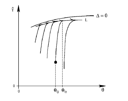
Figure 14: Qualitative structure of the field of integral curves. We see that the calculations in the direction of increasing $\theta$ are stable because of the attraction to the limiting surface $L.$ The surface $L$ is a separatrix – it separates the colliding streams of integral curves. The stream from the $\Delta=0$ surface repulses the curves which come from the ”thickness” (from the distant region; see the text) to this surface. Since the ratios $v_{\theta}/c$ and $\sqrt{2T_{S}/m_{p}}/c$ are small, the relative gap (for example, $\Delta\hat{T}/\hat{T})$ between the $L$ and $\Delta=0$ surfaces is small.

Thus, any trajectory consists of steep and gentle segments (see Fig. 14). The steep and gentle segments lie in the distant and boundary subregions, respectively. On the steep segment, the first and second of the three terms in Eq. (3.17) are important. On the gentle segment, all three terms are comparable. On the steep segment, $\Delta$ rapidly decreases with increasing $\theta.$ As one makes a transition from the steep segment to the gentle one, the decrease in $\Delta$ becomes saturated. The derivative $|d\ln\Delta/d\theta|$ is small on the gentle segment, implying that the radiative losses are roughly offset by the frictional heating. On the steep segment, the energy balance, if by the energy balance we mean the equality of the right part of Eq. (3.17) to zero, is not maintained – the radiative losses are small compared to the heating. This implies that the left part of Eq. (3.17) plays an important role here. Note that the term in the left part corresponds to the advective transfer of radiative enthalpy [cf. Subsec. 1.3 (IV)]. The extent of the steep segment with large (in magnitude) derivatives is small: $\Delta\theta\ll\theta_{\star},$ $\;\Delta\theta=\theta_{tr}-\theta_{0},$ where $\theta_{tr}$ refers to the transition from the steep segment to the gentle one on a given trajectory (see Fig. 14). When the complete system is calculated numerically, the short steep segment is traversed in small steps (a fraction of $\Delta\theta),$ while the extended gentle segment is traversed with large steps (a fraction of $\theta_{\star}).$ At $\theta\approx\theta_{tr},$ the trajectory makes a sharp turn. As can be seen, the trajectories are attracted or caught in the boundary subregion, which lies near the $\Delta=0$ surface and do not leave this subregion. For this reason, the ”levitation” surface is called the attracting or limiting surface, hence the stability of the calculations and the relative ”crudeness” of the results with respect to $U_{0}$ and $\hat{T}_{0}$ and, consequently, with respect to the disk parameters.

Thus, the steep segments along with the distant subregion turn out to be unimportant. Only the boundary subregion remains. Accordingly, we can immediately take the initial data near the curve (3.16). In this way we further narrow down (for the third time, see above) the set of initial data $(\theta_{0},U_{0},W_{0},\hat{T}_{0}).$

Let us introduce the polar (angle/radius) coordinates in the $(U_{0},\hat{T}_{0})$ plane instead of the $U_{0}$ and $\hat{T}_{0}$ coordinates. Let the angle be related to the ratio

$$i=\sqrt{\hat{T}_{0}}/U_{0}.$$

We use the deviation $\delta\Delta$ from the hyperbola (3.16) instead of the radius. One parameter $i$ (3.18) now runs the set of initial data, because the deviation $\delta\Delta$ is insignificant. A certain trajectory (steady accretion flow) corresponds to each value of $i.$ We thus arrive at a one-parameter family of solutions, which we will call the $1d$ family. In phase space, the integral curves from this family cover the surface $L$ near the $\Delta=0$ surface (see Fig. 14).

3.6 Within the One-Parameter Family. The Dependence on Latitude. Critical Regime

Consider an arbitrary steady flow from the family of solutions for a given $\dot{M}$ but with different $i.$ It represents the $\theta-$distribution of $U,W,$ and $\hat{T}.$ Let us study this flow. There are two characteristic regions above and below $\theta_{\star}.$ The lower region is the radiating belt. In this belt, $[W(\theta)]^{2}$ is great; the loss of rotational energy maintains the radiative flux $q(\theta)$ at such a level that $\Delta\ll 1$ (or $q\approx q_{eff};$ see Sec. 1). The rotational energy is exhausted inside the belt. As a result, the luminosity $q(\theta)$ abruptly decreases in the transition zone at $\theta\approx\theta_{\star}$ – the accretion-flow surface darkens. Concurrently, the function $\Delta(\theta)$ increases $[\Delta(\theta)\approx 1$ for $\theta>\theta_{\star}],$ $g_{wr}$ is large $(g_{wr}\approx g_{0}),$ and the layer under the strong press contracts and becomes very thin outside the radiating belt $(h$ is a few centimeters).

The lower (in latitude) region is of greatest interest. Since the radiation pressure in this region is large, the speed of sound $c_{s}\simeq\sqrt{p/\rho}$ is high compared to the meridional spread velocity $v_{\theta}.$ For this reason, the meridional distributions inside the radiating belt become hydrostatic.

In any solution from the family of solutions, the Mach number,

$$\mathop{\rm Ma}\nolimits_{\theta}=\frac{v_{\theta}}{c_{s}},\;\;\;\;\;\;\;c_{s}^{2}=\frac{c^{2}}{3}\,\left(1+\frac{3}{4}\,\frac{\rho_{S}\,c^{2}}{aT_{S}^{4}}\right)^{-1}+\frac{10}{3}\,\frac{T}{m_{p}},$$

which was calculated for a radiation-dominated plasma (Weinberg 1972), must increase with $\theta$ (the pressure decreases, and the flow accelerates). Indeed, the quantity (2.11) decreases with increasing $\theta,$ because its gradient counteracts the tangential component of the centrifugal force, which tends to return the plasma to the equator [see Eq. (2.20)].

Let us compare the $\theta$ dependences for various values of $i$ that run the family. The Mach number $\mathop{\rm Ma}\nolimits_{\theta}$ (3.19) at the interface between the disk and the spread layer $[\mathop{\rm Ma}\nolimits_{\theta}(\theta=0)]$ is smaller, if $i$ is larger $[i$ is the reciprocal of the Mach number without a factor $\simeq\sqrt{G_{eff}/\Delta};$ cf. the definitions (3.18) and (3.19)]. We take $\mathop{\rm Ma}\nolimits_{\theta}(\theta_{0})$ at the interface between the disk and the spread layer and assume that the disk is thin $(\theta_{0}\ll\theta_{\star}).$ We can thus write $\mathop{\rm Ma}\nolimits_{\theta}(\theta=\theta_{0})=\mathop{\rm Ma}\nolimits_{\theta}(\theta=0).$ At a fixed $i,$ the function $\mathop{\rm Ma}\nolimits_{\theta}(\theta)$ monotonically increases with $\theta$ in the interval $0<\theta<\theta_{\star}.$ Consequently, $\mathop{\rm Ma}\nolimits_{\theta}(\theta)$ reaches a maximum in this interval at its edge. An analysis of the effect of $i$ shows that $\mathop{\rm Ma}\nolimits_{\theta}(\theta_{\star}),$ together with $\mathop{\rm Ma}\nolimits_{\theta}(0),$ increases with decreasing $i.$ On the $i$ axis, the family fills the semiaxis $i_{\star}<i<\infty.$ The edge $i_{\star}$ corresponds to the critical spread regime, in which the sonic point $\theta_{c}$ lies at the boundary of the radiating belt $[\,\theta_{c}=\theta_{\star},\;\mathop{\rm Ma}\nolimits_{\theta}(\theta_{\star})\simeq 1\,].$ $\mathop{\rm Ma}\nolimits_{\theta}(\theta)$ also monotonically increases with $\theta$ for $i<i_{\star}.$ If $i<i_{\star},$ then the rotational energy at $\theta_{c},$ at which $\mathop{\rm Ma}\nolimits_{\theta}(\theta_{c})\simeq 1,$ has not yet been exhausted: $v_{\varphi}(\theta_{c})>0,$ i.e., the latitude $\theta_{c}$ is inside the radiating belt. At the sonic point $\theta_{c},$ the solution becomes two-valued (’tips over’). Accordingly, we reject the solutions with $i<i_{\star}$ as nonphysical.

The critical regime occupies a special place. It restricts the $1d$ family of subsonic (for $\theta<\theta_{\star})$ flows. In this regime, the plasma is ejected with the speed of sound from the radiating belt. Accordingly, the region at $\theta>\theta_{\star}$ has no effect on the flow in the radiating belt. At $i>i_{\star},$ the regions $\theta<\theta_{\star}$ and $\theta>\theta_{\star}$ are coupled. For example, the action of lateral forces (and friction $\tau_{\theta})$ between elements $\delta\theta$ extends from the region $\theta>\theta_{\star}$ into the region $\theta<\theta_{\star}.$

4 PHYSICS OF DECELERATION AND SPREAD

4.1 Numerical Simulations

The system (3.12)-(3.14) was integrated numerically. In doing so, we approximated the derivatives by finite differences. We specified $i$ to calculate the initial point and found the intersection point with the coordinates $(U_{01},\hat{T}_{01})$ of the curves $i=i(U,\hat{T})$ and $\Delta(U,\hat{T})=0.$ We took $U_{0}=0.9U_{01}$ and $\hat{T}_{0}=0.9\hat{T}_{01}$ as the initial values. The values of $\theta_{0}$ and $W_{0}$ were varied $(10^{-3}<\theta_{0}<10^{-2},$ $10^{-3}<1-W_{0}<10^{-1}).$ The steep segment was traversed with the step $\sim 10^{-6}\Delta\theta.$ We took $\theta,U,W,$ and $\hat{T}$ at its end as the initial values when we calculated the gentle segment with a step $\sim 10^{-6}\theta_{\star}.$ The round-off error was $10^{-16}$ (double accuracy). A preliminary estimate of $\theta_{\star}$ was obtained from formula (1.1)’ for the Eddington scale.

The family consists of subsonic (subcritical) and supersonic (supercritical) subfamilies in the radiating belt. In the solutions from the supercritical subfamily, the sonic point lies inside the radiating belt (see Subsec. 3.6). As was stated, these solutions are discarded.

When we say below that the flow is subsonic, we mean that it is subsonic in the radiating belt. The determinant $d(\theta)$ (3.15) was calculated along an integral curve. The first zero of the function $d(\theta),$ when running in $\theta$ from $\theta_{0},$ is called the sonic point $\theta_{c}.$ At this point, the integral curve makes a turn, and the solution becomes two-valued. Since the determinant $d$ appears in the denominator of the derivatives (3.12) and (3.14), the derivatives $U^{\prime}$ and $\hat{T}^{\prime}$ have a singularity at $\theta_{c}.$ Thus, the solution exists in the interval $\theta_{0}<\theta<\theta_{c}.$

4.2 One-Parameter Family as a Whole and the Passage Through the Critical Point

As was shown in Subsecs. 3.4-3.6, the integral curves with general initial data form a one-parameter (or $1d)$ family. An example of a family is given in Fig. 15 $(\mathop{\rm Ma}\nolimits_{\theta}$ profiles, transcritical and supercritical solutions, $100<i<160)$ and Fig. 16 $(\Sigma_{S}$ profiles in the same family, subcritical and supercritical solutions, $100<i<500).$ At a fixed $\theta,$ $\;\mathop{\rm Ma}\nolimits_{\theta}$ increases, while $\Sigma_{S}$ decreases with decreasing $i.$ In Fig. 15, the upper and lower solutions refer to $i=100$ and $160,$ respectively. In Fig. 16, the upper and lower solutions refer to $i=500$ and $100,$ respectively. The supercritical solutions terminate at $\theta_{c}<\theta_{\star}.$ The subcritical solutions extend into the region $\theta>\theta_{\star},$ i.e., their termination point $\theta_{c}$ lies to the right of $\theta_{\star}.$ In Figs. 15 and 16, the two upper (Fig. 15) and two lower (Fig. 16) solutions are supercritical. The arrow in Figs. 15 and 16 marks the critical solution with $i=i_{\star}$ and $\theta_{c}=\theta_{\star}.$ In Fig. 15, the subcritical solutions with $i>i_{\star}$ run below (above in Fig. 16) this solution. The solutions for which $i$ lies in the vicinity of the critical value $i_{\star}$ $\;(|i-i_{\star}|\ll i_{\star}).$ are called transcritical.

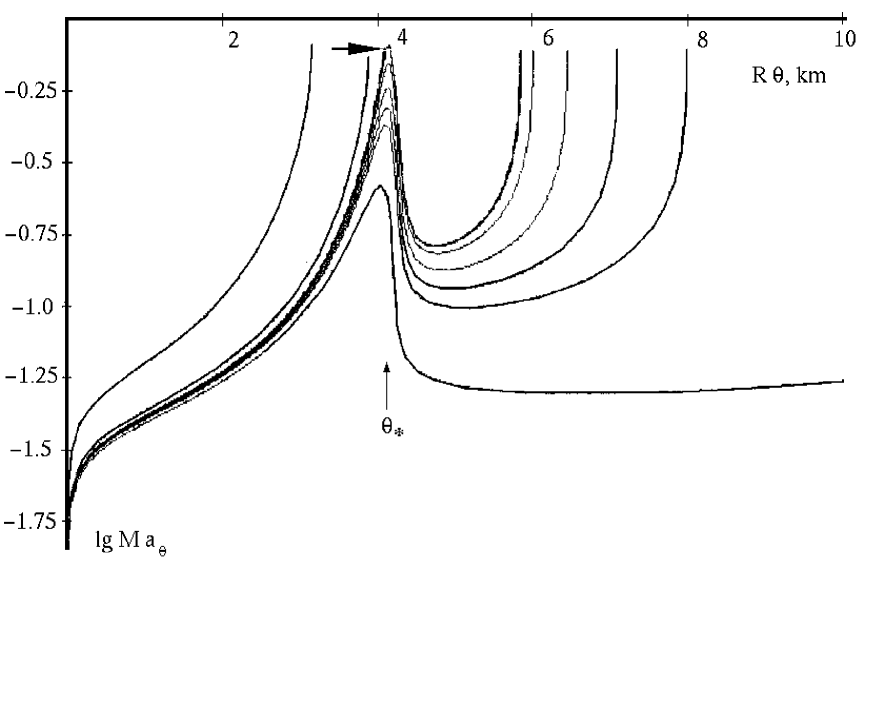
Figure 15: One-parameter family of steady spread flows $(100<i<160).$ The dependences $\log[\mathop{\rm Ma}\nolimits_{\theta}(R\theta)]$ are for $\dot{M}=4\cdot 10^{17}$ g s${}^{-1},$ $1-W_{0}=10^{-2},$ $\;\theta_{0}=10^{-3},$ and $\alpha_{b}=10^{-3}.$ $R\theta$ is the arc length along the meridian in km, $R$ is the stellar radius. Here $R=10$ km and $M=1.4M_{\odot}.$ The calculations were performed using Newton’s approximation. Recall that the curves terminate at the sonic point $\theta_{c},$ at which the determinant is $d(\theta_{c})=0$ [see Eq. (3.15) and Subsec. 4.1], or are bounded by the computational interval.

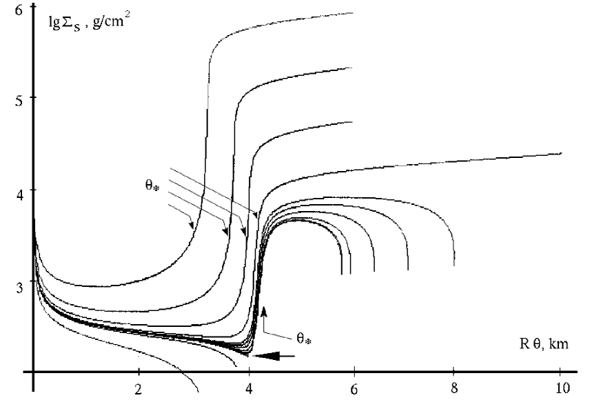
Figure 16: $\Sigma_{S}$ profiles for various values of $i.$ The four upper profiles rest on the end of the computational interval. The remaining profiles terminate at the sonic point. The parameters of the variant are given in the caption to Fig. 15.

Let us discuss the transcritical behavior. The function $\theta_{c}(i)$ increases with increasing $i$ (see Fig. 17 and Figs. 15 and 16). This function appears to have a discontinuity at $i_{\star}.$ In our example, $i_{\star}\approx 151.404.$ At least in our example at the accuracy we chose $(1.5-$mm step), the discontinuity cannot be reduced by refining $i$ $\;(i_{-}=151.403,\;i_{+}=151.405).$ The discontinuity boundaries in $R\theta$ are: $R\theta_{-}=4.1365$ and $R\theta_{+}=5.8448$ km; the relative width is $\Delta\hat{\theta}=$ $2(\theta_{+}-\theta_{-})/(\theta_{+}+\theta_{-})=0.34.$

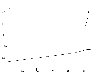
Figure 17: Passage of the sonic point $\theta_{c}$ through latitude $\theta_{\star}$ as $i$ is varied (3.18). The latitude $\theta_{c}$ is given in degrees. The parameters of the variant are given in the caption to Fig. 15.

The latitude $\theta_{\star}$ divides the flow into two characteristic regions (Sec. 1 and Subsec. 3.6). It separates the rotating (separation in $W),$ hot (separation in $\hat{T}),$ levitating (separation in $\Delta$ and $h),$ and radiating (separation in $q)$ region from the nonrotating, cold, pressed and dark region. The separation into these regions is clearly seen on the subsonic profiles in Figs. 15 and 16 (see the arrows $\theta_{\star}).$ The transition between them is sharp. We can also determine $\theta_{\star}$ from the left boundary of the discontinuity in Figs. 15 and 16 (see also Fig. 17). It is marked by the arrow in Figs. 15-17. The discontinuity in $\theta_{c}(i)$ is produced by the passage of the sonic point through the belt boundary $\theta_{\star}.$

In the momentum equation (3.5), the momentum flux in the subsonic flow is small compared to the pressure gradient. The gradient is balanced either by the component of the centrifugal force $F_{cf}$ or by the meridional friction $F_{\theta}.$ Calculations show that the meridional friction $F_{\theta}$ and the force $F_{cf}$ can be disregarded inside and outside the radiating and rotating belt, respectively. This is yet another characteristic in which there is a clear separation at $\theta_{\star}.$

Dark part of the layer. The sonic point and its position. In the dark region, the system (3.5)-(3.7) simplifies greatly. Here, we may assume that $\Delta=G_{eff}=1$ and ignore the rotation of matter. The flow as a whole (the radiating and dark layers) is numerically analyzed below. The numerical analysis must be preceded by a qualitative study. Since the variability of $\cos\theta$ in the equations is of little importance for a qualitative analysis, we set $\cos\theta=1.$ The qualitative analysis leads us to conclude that the flow terminates at the sonic point, as confirmed below by the numerical calculations which are free from the assumed simplifications. This conclusion is important in constructing the ensuing theory of slow spread and settling of matter over a neutron-star surface, because in this way the radiative-frictional mechanism of spread deceleration is revealed.

As a result of the simplifications above, we obtain

$$(5U^{2}-4\hat{T})U^{\prime}+4U\,\hat{T}^{\prime}=-5\alpha_{b}U^{3}/\hat{T},$$

$$5UU^{\prime}+14\hat{T}^{\prime}=-5A\,U\,\hat{T}^{4}.$$

Resolving the system (4.1), (4.2) for the derivatives, we obtain

$$U^{\prime}=10U^{2}(2A\hat{T}^{5}-7\alpha_{b}U)/\hat{T}d_{1},$$

$$\hat{T}^{\prime}=5U[\,(4\hat{T}-5U^{2})A\hat{T}^{5}+5\alpha_{b}U^{3}]/\hat{T}d_{1},$$

$$d_{1}=50U^{2}-56\hat{T}.$$

Eliminating $\theta$ from the system (4.3), (4.4), we arrive at the equation

$$\frac{d\hat{T}}{dU}=\frac{(4\hat{T}-5U^{2})(A/\alpha_{b})\hat{T}^{5}+5U^{3}}{2U\,[\,2(A/\alpha_{b})\hat{T}^{5}-7U\,]}$$

in the phase plane, which allows an effective qualitative analysis, because it is two-dimensional.

Let us estimate the ratio of the frictional $(\alpha_{b}U)$ and radiative $(A\hat{T}^{5})$ terms in Eq. (4.6). For $\dot{M}_{17}\sim 1,$ $\;\alpha_{b}\sim 10^{-3},$ $\;T\simeq 0.5$ keV, $U\sim\sqrt{\hat{T}}$ they are comparable. We offset the large $(\sim 10^{23})$ constant $A/\alpha_{b}$ by changing the scale

$$U\to\sqrt{\lambda}\hat{U},\;\;\;\;\;\;\;\hat{T}\to\lambda\tilde{T},\;\;\;\;\;\;\;\lambda=(\alpha_{b}/A)^{2/9}=2.7\cdot 10^{-5}\,\alpha_{b}^{2/9}\,\dot{M}_{17}^{4/9},$$

[see (3.9) and (3.11)]. Note that the velocity and temperature at $\hat{U}=\tilde{T}=1$ are $v_{\theta}=330\,\alpha_{3}^{1/9}\,\dot{M}_{17}^{2/9}$ km s^-1 and $\,T=0.57\,\alpha_{3}^{2/9}\,\dot{M}_{17}^{4/9}$ keV, where we set $\alpha_{b}=10^{-3}\alpha_{3}.$ Replace $\hat{U},\tilde{T}$ by $\mathop{\rm Ma}\nolimits_{\theta},\tilde{T}.$ In the dark flow, we have $\mathop{\rm Ma}\nolimits_{\theta}^{2}=(3/5)\hat{U}^{2}/\tilde{T}$ [see (3.19)]. Making the replacements $X=\sqrt{10/9}\mathop{\rm Ma}\nolimits_{\theta}$ and $Y=\tilde{T}^{9/2},$ we can smooth out the fourth power of temperature from Stefan-Boltzmann’s law, which complicates the analysis. In these variables, Eq. (4.6) takes the form

$$\frac{dY}{dX}=9\,\frac{Y}{X}\;\frac{\sqrt{2/3}(8-15X^{2})Y+15X^{3}}{\sqrt{2/3}(8+15X^{2})Y-56X-15X^{3}}.$$

A phase portrait of Eq. (4.7) is shown in Fig. 18. The function $[X]_{c}(i)=X[\theta_{c}(i)]=X(i)$ gives the Mach number at the end of the integral curve (at the sonic point). It is constant $[X(i)\equiv\sqrt{56/75}]$ at $i>i_{\star},$ i.e., when the sonic point lies in the dark region. In the radiating region, in which $i<i_{\star}$ and $\theta_{c}<\theta_{\star},$ this function slightly changes with $i.$ For $100<i<i_{\star},$ $\;X(i)$ is smaller than $\sqrt{56/75}$ by $5\%$ and abruptly increases to this value at $i_{\star}.$ The vertical line 4 $\;(X=\sqrt{56/75})$ in Fig. 18 is a locus of sonic points $\theta_{c}.$ On this line, the determinants $d$ (3.15) and $d_{1}=\lambda\,\tilde{T}(75X^{2}-56)\,$ (4.5) vanish. It is easy to show that the vertical line 4 and the isoclines of zeros (curve 2) and infinities (curve 1) intersect at a single point.

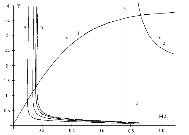
Figure 18: Phase plane of Eq. (4.7): 1 – the isocline of infinities, the arrows indicate the orientation of integral curves on the isoclines; 2 – the isocline of zeros; 3 – its asymptotic limit for $Y\to\infty,$ 4 – the sonic point $(d_{1}=0,$ $\;\mathop{\rm Ma}\nolimits_{\theta}=\sqrt{56/75}).$ The integral curves 5 were taken from the calculations of the complete system which are shown in Figs. 15-17 (the subsonic subfamily, $i>i_{\star}).$

It follows from the qualitative analysis of Eq. (4.7) that the integral curves which start from the subsonic region must necessarily intersect the vertical line 4. Indeed, the segment of the integral curve at $\theta>\theta_{\star}$ starts from the subsonic region. The derivative $dY/dX$ (4.7) is positive above the isocline of infinities at $X<\sqrt{8/15},$ while the derivative $dY/d\theta$ is negative [see Eq. (4.4)]. Hence, on the integral curve in the $X,Y$ plane, the motion occurs in the direction of decreasing $Y$ and $X$ as $\theta$ increases. The $Y$ semiaxis cannot be intersected. The integral curve 5 must then necessarily intersect the isocline of infinities (see Fig. 18). Below the isocline of infinities, $dY/dX$ is negative. This time the $X$ semiaxis cannot be intersected. The isocline of zeros 2 lies behind the ”triangle” that is formed by the segments of the $X$ semiaxis, the vertical line 4, and the isocline of infinities 1. Therefore, the stream of integral curves 5 arrives at the vertical line 4. The curves crowd together near the limiting curve that corresponds to $i_{\star}.$ The initial value of $X$ (or $\mathop{\rm Ma}\nolimits_{\theta})$ decreases with increasing $i.$ Thus, we established the causes of the ”tipping” and determined the position of the sonic point in the dark region by analyzing the simplified system (4.1) and (4.2).

4.3 Preference of the Critical Regime. The Pedestal Under the Radiating Belt

In Figs. 1-4 we assumed that the surface $S$ is equipotential (”horizontal”). The equipotential surface of a nonrotating star is spherical. Let us find out whether the underlying surface can be spherical. Calculations show that the surface density $\Sigma_{S}(\theta)$ of the plasma which constitutes the spreading layer is higher in the dark region (Fig. 10). In addition, the acceleration $g_{eff}=[\,1-U^{2}(\theta)-W^{2}(\theta)\,]\,g_{0}$ in a differentially rotating radiating belt is smaller than that in the dark region. Consequently, the weight $g_{eff}(\theta)\,\Sigma_{S}(\theta)$ of the spreading layer per unit area is larger in the dark region; the pressure of the spreading layer on the underlying layers is also higher. We ignore the motion in the underlying layer beneath the surface $S.$ Since the motion in this layer is strongly subsonic, the hydrostatic contribution to the pressure is more important than the dynamical contribution. Because of the difference in pressure on the surface $S$ from the spreading layer under the radiating region, this surface rises to form a pedestal. Let $h_{US}(\theta)=R_{S}(\theta)-R_{S}(90^{0}),$ where $R_{S}$ is the radius of this surface. We have

$$(h_{US})_{hs}=\frac{p_{d}-p_{b}}{\rho_{US}\;g_{0}}\simeq\frac{p_{d}/\rho_{US}}{g_{0}}\simeq\frac{(c_{s})_{US}^{2}}{g_{0}}\simeq 17\,T_{US},$$

because there is no rotation under $S$ and because the total pressing force $g_{0}$ is in action. Here, $p_{d}$ and $p_{b}$ are the pressures on the surface $S$ under the dark and radiating regions, respectively; $\rho_{US}$ is the density of the matter under $S;$ $(c_{s})_{US}$ and $T_{US}$ are the speed of sound and the temperature under $S;$ and $h_{US}$ and $T_{US}$ are given in cm and keV, respectively.

In addition, the radiating belt is considerably hotter with $T_{US}(\theta)=T_{S}(\theta)$ (see Subsec. 2.1). As noted above, the radiating belt heated up the underlying layers, causing the pedestal height to increase by $(h_{US})_{T}\simeq(c_{s})^{2}_{S}/g_{0}.$

Let us compare the height $(h_{US})_{hs}+(h_{US})_{T}$ with the thickness

$$h_{eff}(\theta)=\frac{1}{|(d\ln\rho/dy)_{S}\,|}=\frac{4}{3}\;\frac{R\;\hat{T}}{\Delta}$$

of the spreading layer, (see Fig. 5). We see that the thickness of the spreading flow in the radiating belt is much larger than the pedestal height. This is because $g_{wr}$ and $g_{0}$ differ. Consequently, the relief of the surface $S$ is not important for the flow in the radiating belt.

At the same time, the height $h_{US}(0)$ is of the order of the thickness of the spreading dark layer, implying that the dark flow cannot affect the flow in the radiating belt. The flow in the belt must therefore be transcritical.

4.4 Spread of Dark Matter

The dark flow is specified by the functions $v_{\theta}$ and $T_{S}.$ Its segment $\theta_{\star}<\theta<\theta_{c}$ terminates at the sonic point (see Subsec. 4.2). The separation $\theta_{c}-\theta_{\star}$ increases with a decreasing initial Mach number, for example, $\mathop{\rm Ma}\nolimits_{\theta}(\theta_{\star}).$ In order to reach the pole $(\theta_{c}>90^{0}),$ it is necessary that $\mathop{\rm Ma}\nolimits_{\theta}(\theta_{\star})$ be sufficiently small.

In the model (3.2)-(3.4), the surface $S$ is impenetrable [integral (3.1)]. Above this surface, the newly accreted matter is transported from the source at the equator to the sink. Let us consider the sink. The dark layer is thin compared to the stellar radius, $h\ll R.$ It may mix with the underlying fluid when traversing a long path, $(s_{mix}-s_{\star})/h\gg 1;$ the boundary $S$ terminates in the mixing zone.

In another case, the mixing is ineffective, and the dark flow runs up to the pole. In this case, we have a ”bath-filling” flow with a filling ”tap” near the boundary $\theta_{\star}.$ The mixing zone then is located not far from the tap: $s_{mix}-s_{\star}$ is of the order of $(10-100)h.$ In the ”bath”, the matter is essentially in hydrostatic equilibrium and, naturally, moves at velocities much lower than the speed of sound. This matter flows under the radiating belt (especially since the pressure under the radiating layer is lower than the pressure under the dark layer; see Subsec. 4.3). The boundary $S$ is preserved under this belt. The ”bath” filling is very slow, and the flow is strongly subsonic. Accordingly, the weight contribution $(h_{US})_{hs}$ to the pedestal vanishes, and only the temperature contribution $(h_{US})_{T}$ remains. Note the possibility of subsonic circulation under $S$ not only due to the viscous entrainment (gripping) by the high-velocity layer (see Subsecs. 1 and 2.1) but also due to the difference in the heights of equal pressure. In the Earth’s atmosphere, this leads to trade-wind circulation which is attributable to solar heating of the equatorial zone (Palmen and Newton 1969; Bubnov and Golitsyn 1995). The filling causes the fluid to rise at the velocity $v_{a}$ or to settle at the same velocity. This is the radial component of the total velocity. It is easy to see that $v_{a}\simeq(1/2)(h/R)(\rho_{S}/\rho_{US})\,v_{\theta}$ is small compared to the spread velocity $v_{\theta}$ in the radiating belt – the matter traverses the belt rapidly but settles slowly. At the parameters of the problem under consideration, $v_{a}\sim 10$ m s${}^{-1}.$ Such velocity ensures a uniform increase in the surface density over the entire stellar surface. A particular regime of the motion of the dark fluid affects the dynamics of a loose belt only slightly. Accordingly, the approach (3.1)-(3.4) is acceptable for describing the belt all the way to the pole. Of course, flows which run up to the pole require a special analysis. It is necessary to introduce the parameter $v_{a},$ change the boundary condition downstream, and add the equation for $\Sigma_{S}$ to the system (3.2)-(3.4) instead of the integral (3.1). Note also that the allowance for the moderate penetrability of the surface $S$ under the radiating and rotating belt results in certain quantitative changes, although qualitative conclusions remain valid. This can be seen from the results (see below) on the effect of variations in the accretion rate $\dot{M}$ on the belt structure.

4.5 Effect of Friction

Since the intensity of radiation cooling cannot exceed the Eddington limit, the area of the emitting surface must be large enough to remove the released heat [see (1.1), (1.1)’, (1.2), (1.2)’]. The system under study has excess energy, if the emitting area is larger than the area of the disk base. The disk accretion in the disk-layer transition zone then gives way to the spread of matter over the stellar surface. The flow boundary ( in the plane that passes through the polar axis) turns $90^{0}$ in the transition zone (see Figs. 1-4 and Sec. 1). In this case, the radial flow (disk, $|v_{r}|\gg v_{\theta})$ transforms to the meridional flow (spread, $|v_{r}|\ll v_{\theta}).$ Because of the delay in the deceleration, a reservoir filled with fluid which retains its rotation carried from the disk is formed. Its surface emits radiation (radiating belt).

To assess the role of the friction model, we varied the coefficient $\alpha_{b}$ in (2.16). The cases with $\alpha_{b}=10^{-3}$ and $10^{-3}/3$ are compared in Fig. 19. The transcritical profiles, which refer to the discontinuity boundaries $i_{-}$ and $i_{+},$ are shown in this figure (see Subsec. 4.2). Let us compare the transcritical profiles for these values of $\alpha_{b}.$ The critical value of $i_{\star}$ increases roughly proportional to $1/\alpha_{b}$ (by a factor of 2.7). The functions $\mathop{\rm Ma}\nolimits_{\theta}(\theta)$ and $U(\theta)$ decrease, while $\Sigma_{S}(\theta)$ increases $\propto\alpha_{b}$ and $\propto 1/\alpha_{b},$ respectively. The value of $\theta_{\star}$ increases by $6\%.$ The functions $W(\theta)$ are virtually equal, differing by only fractions of a percent. Consequently, the $q(\theta)$ profile [see (1.2)] is invariant to $\alpha_{b}.$ The bottom temperature $T_{S}$ rises $\propto(1/\alpha_{b})^{1/4}$ due to the increase in $\Sigma_{S}$ [see (2.14)].

Figure 19: Response of the function $q(\theta)$ to variations in $i$ and $\alpha_{b}.$ Curves 1, 2, and 3 refer to moderately supersonic (1), slightly subsonic (2), and moderately subsonic (3) spread regimes for $\alpha_{b}=10^{-3.}$ Curve 4 gives a subsonic transcritical profile for $\alpha_{b}=10^{-3}/3.$ We see that variations in $\alpha_{b}$ affect the $q$ profile only slightly.

The degree of levitation is $\Delta\simeq 10^{-3}-10^{-2},$ since it responds to a variation in $\alpha_{b}$ in the same way $T_{S}$ does. The height $h_{eff}$ (see Subsec. 4.3) is invariant to $\alpha_{b}$ variation with the same accuracy as $W.$

As can be seen, there are parameters which change significantly as $\alpha_{b}$ is varied (these include $i_{\star},$ $U,$ $\mathop{\rm Ma}\nolimits_{\theta},$ $\Sigma_{S})$ and parameters which change weakly $(T_{S},\Delta,\theta_{\star})$ or only slightly $(h_{eff},W,q).$ Note that in view of the behavior noted above, the tangential stress (2.16) belongs to the parameters which respond only slightly, because $\rho_{S}=(4/3)\Sigma_{S}/h_{eff}\propto 1/\alpha_{b}.$ This also follows from Eqs. (2.22) and (3.3) and from the invariance of $W(\theta).$ The width of the discontinuity in $\theta_{c}$ at $i_{\star}$ $\;(\Delta\hat{\theta},$ see Subsec. 4.2) depends on $\dot{M}$ and $\alpha_{b}.$

4.6 Effect of Initial Parameters

It is clear from the arguments which lead to formula (1.2) that the equatorial part of the rotating belt radiates weakly, because the normal component of the centrifugal force is large here. Thus, there are two bright belts at latitudes $\theta_{\star}$ and $-\theta_{\star}.$ The greatest brightness is reached near the edge of the radiating belt. The maximum is appreciably lower than unity, because where $W\simeq 1,$ the subtraction of the centrifugal component is significant and where $W$ is small, there is nothing to radiate. It follows from the smallness of $\Delta$ compared to $G_{eff}$ that $q\approx q_{eff}$ [see Sec. 1 for a discussion of formula (1.2)].

Let us analyze the effect of the initial parameters $W_{0}$ and $\theta_{0},$ associated with the disk, on the results. We compare the cases with $1-W_{0}=10^{-2}$ and $10^{-1.}$ They correspond to a change in the deviation of the rotation velocity from the Keplerian velocity by an order of magnitude. For this change in $W_{0},$ the kinetic energy increases by $2\%,$ $i_{\star}$ increases by $42\%,$ the belt width $\theta_{\star}$ increases by $3\%,$ $\mathop{\rm Ma}\nolimits_{\theta}$ inside the belt decreases by $12\%,$ the surface density $\Sigma_{S}$ increases by $7\%,$ the rotation velocity $W$ increases by $1.4\%,$ the temperature rises by $0.8\%,$ the degree of levitation $\Delta$ decreases by $13\%,$ the height $h_{eff}$ increases by $14\%,$ and $q$ decreases by $3\%.$

Let us increase the meridional extent of the disk base by a factor of 10: $\theta_{0}=10^{-3}$ is replaced by $10^{-2.}$ The critical value of $i_{\star}$ increases by $8\%.$ The distributions of $\mathop{\rm Ma}\nolimits_{\theta},\Sigma_{S},W$ and other variables for disks of thickness $2R\theta_{0}=20$ and 200 m differ only slightly. The distribution in $\theta$ seems to shift by an amount of the order of the difference between the values of $\theta_{0}.$ Thus, for $1-W_{0}\ll 1$ and $\theta_{0}\ll\theta_{\star},$ variations in $W_{0}$ and $\theta_{0}$ have a marginal effect on the results, in particular, on the $q(\theta)$ profile.

4.7 Dependence on Accretion Rate

Above, we discussed the main points regarding variations in $\alpha_{b},$ $W_{0},$ and $\theta_{0}.$ Let us now study the effect of $\dot{M}.$ The critical value $i_{\star}(\dot{M})$ and the belt width $\theta_{\star}(\dot{M})$ are plotted versus the accretion rate in Fig. 20. In the calculations, we approached the critical value by compressing the transcritical vicinity by the fork method (see Subsecs. 3.6, 4.2, 4.3). The width $\theta_{\star}(\dot{M})$ was determined from the last calculated supercritical profile. We took the position of the sonic point in this profile as the belt width. An analysis of the effect of variations in $\dot{M}$ on the spread-flow structure shows that the relative discontinuity width $\Delta\hat{\theta}$ (Subsec. 4.2) decreases with increasing $\dot{M}.$ At $\dot{M}\approx\dot{M}_{pole},$ the discontinuity disappears, and the dependence on $i$ becomes smooth; the edge of the radiating belt comes close to the pole. Under these conditions, the edge of the rotating belt was taken as $\theta_{\star}(\dot{M}).$ We chose the smallest value of $i$ at which this edge lies at a distance from the pole and took it as $i_{\star}.$

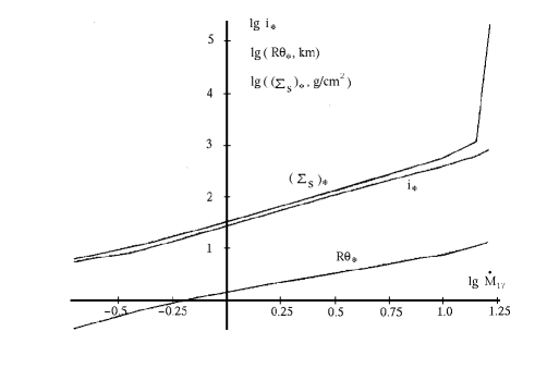
Figure 20: Critical value of $i_{\star},$ radiating-belt width $R\theta_{\star},$ and surface density $(\Sigma_{S})_{\star}$ at the belt boundary versus $\dot{M}.$

In Fig. 20, we also plotted $(\Sigma_{S})_{\star}$ versus $\dot{M}.$ The value of $(\Sigma_{S})_{\star}$ is $\Sigma_{S}(\theta_{\star}),$ where $\theta_{\star}$ was determined from the last calculated supercritical profile. Near the point of stoppage at the pole for $\dot{M}\approx M_{pole},$ we took the edge of the rotating belt as $\theta_{\star}.$ The function $(\Sigma_{S})_{\star}(\dot{M})$ begins to rapidly increase near the pole. It is physically clear that after the point of stoppage of the loose radiating belt at the pole, the spread of matter slows down greatly (Subsec. 4.4). The slowdown causes the surface density $\Sigma_{S}$ to increase proportionally. The power law fitting the dependences are $i_{\star}\approx(\Sigma_{S})_{\star}$ [g cm${}^{-3}]$ $\approx 35\dot{M}_{17}^{1.14},$ $\;R\theta_{\star}=s_{\star}$ [km] $\approx 1.4\dot{M}_{17}^{0.8}.$

Let us define the contrast as the ratio of $\Sigma_{S}$ in the central zone to $(\Sigma_{S})_{\star}.$ The contrast increases with increasing $\dot{M}.$ The fact that it is greater than unity is attributable to the existence of a strongly subsonic central zone. For this reason, the spreading layer stretches when it approaches the edge of the radiating belt. While at large $\dot{M}$ there are a subsonic center and a transonic edge, at small $\dot{M}$ the entire radiating belt is transonic.

4.8 Limiting Magnetic Field

Let us estimate the magnetic-field strength that still has no effect on the pattern of deceleration and spread outlined above. Compare the magnetic pressure $H^{2}/8\pi$ and the pressure $p_{S}=g_{eff}\,\Sigma_{S}$ (2.2) at the bottom of the spread layer. To obtain an estimate, we assume that $g_{eff}\sim g_{0}.$ We take $(\Sigma_{S})_{\star}$ as a typical value of $\Sigma_{S}$ and use the fitting dependence on $\dot{M}$ which we derived in Subsec. 4.7. As a result, we obtain $H<H_{max},$ $\;H_{max}=4\times 10^{8}(\dot{M}_{17})^{0.57}$ gauss. A weaker field appears to ”get buried” under the layers of accreting plasma. X-ray bursters give an example of neutron stars with a weak magnetic field.

CONCLUSION

The spread of matter during disk accretion was considered. We found a radiating belt to be formed in a certain range of $\dot{M}.$ The belt width $\theta_{\star}$ depends on $\dot{M}.$ At $L_{SL}/L_{edd}\simeq 3\times 10^{-3},$ the width $\theta_{\star}$ is of the order of the thin-disk thickness $\theta_{0}=10^{-3}\div 10^{-2}.$ The belt disappears at $L_{SL}/L_{edd}\approx L_{pole}/L_{edd}\approx 0.9,$ because the entire stellar surface radiates. The belt rotates. Its rotation velocity depends on latitude. This belt levitates in the sense that the pressing acceleration $g_{wr}$ is small compared to the gravitational acceleration $g_{0}.$ A delay in the deceleration of rotation is responsible for the appearance of the belt. This delay in the deceleration is attributable to a great decrease in the bottom density due to the levitation and loosening of the matter.

REFERENCES

Barret, D., Bouchet, L., Mandrou, P., et al., Astrophys. J., 1992, vol. 394, p. 615.

Bisnovatyi-Kogan, G.S., Mon. Not. R. Astron. Soc., 1994, vol. 269, p. 557.

Boubnov, B.M. and Golitsin, G.S., Convection in Rotating Fluids, Fluid Mech. and its Appl., vol. 29, Dordrecht: Kluwer, 1995.

Campana, S., Stella, L., Mereghetti, S., et al., astro-ph/9803303, 26 Mar, 1998a.

Campana, S., Colpi, M., Mereghetti, S., et al., astro-ph/9805079, 6 May, 1998b.

Chandrasekhar, S., Radiative Transfer, New York: Dover, 1960.

Chugaev, R.R., Gidravlika (Hydralics), Leningrad: Energoizdat, 1982.

Felten, J.E. and Rees, M.J., Astron. Astrophys., 1972, vol. 17, p. 226.

Gilfanov, M., Revnivtsev, M., Sunyaev, R., and Churazov, E., Astron. Astrophys., 1998, vol. 338, p. L83.

Illarionov, A.F. and Sunyaev, R.A., Astrophys. Space Sci., 1972, vol. 19, p. 61.

Illarionov, A.F. and Sunyaev, R.A., Soviet Astron., 1975, vol. 18(4), p. 413.

Landau, L.D. and Lifshitz, E.M., Gidrodinamika (Hydrodynamics), Moscow: Nauka, 1986.

Lapidus, I.I. and Sunyaev, R.A., Mon. Not. R. Astron. Soc., 1985, v. 217, p. 291.

Lin, C.-L., Moeng, C.-H., and Sullivan, P.P., Phys. Fluids, 1997, vol. 9(11), p. 3235.

Loitsyanskii, L.G., Mekhanika zhidkosti i gaza (Fluid and Gas Mechanics), Moscow: Nauka, 1973.

Lynden-Bell, D. and Pringle, J.E., Mon. Not. R. Astron. Soc., 1974, vol. 168, p. 603.

Meyer, F. and Meyer-Hofmeister, E., Astron. Astrophys., 1989, vol. 221, p. 36.

Narayan, R. and Yi I., Astrophys. J., 1995, vol. 452, p. 710.

Palmen, E. and Newton, W., Atmospheric Circulation Systems, N.Y. and London: Academic Press, 1969.

Papaloizou, J.C.B. and Stanley, G.Q.G., Mon. Not. R. Astron. Soc., 1986, vol. 220, p. 593.

Popham, R. and Narayan, R., Astrophys. J., 1995, vol. 442, p. 337.

Popham, R., Narayan, R., Hartmann, L., and Kenyon, S., Astrophys. J., 1993, vol. 415, p. L127.

Pringle, J.E. and Savonije, G.J., Mon. Not. R. Astron. Soc., 1979, vol. 187, p. 777.

Schlichting, H., Grenzschicht–Theorie, Karlsruhe: G. Braun, 1965.

Shakura, N.I. and Sunyaev, R.A., Adv. Space Res., 1988, vol. 8, p. 135.

Shakura, N.I. and Sunyaev, R.A., Astron. Astrophys., 1973, vol. 24, p. 337.

Shakura, N.I., Soviet Astron, 1972, vol. 16(3), p. 532.

Sibgatullin, R.N. and Sunyaev, R.A., Astron. Lett., 1998, vol. 24(6), p. 774. (Astro-ph/9811028).

Sobolev, V.V., Uchenye Zapiski Leningr. Univ., Ser. Matem. Nauk, 1949, vol. 18, issue 116, p. 3.

Spitzer, L., Physics of Fully Ionized Gases, N.Y.: Interscience, 1962.

Sunyaev, G.A. and Shakura, N.I., Soviet Astron. Lett., 1986, vol. 12(2), p. 117.

Sunyaev, R.A. and Titarchuk, L.G., Astron. Astrophys., 1980, vol. 86, p. 121.

Tylenda, R., Acta Astron., 1981, vol. 31, p. 267.

Van der Klis, M., astro-ph/9812395, 22 Dec, 1998.

Weinberg, S., Gravitation and Cosmology: Principles and Applications of the General Theory of Relativity, N.Y. etc.: John Wiley and Sons, 1972.