The Optical Gravitational Lensing Experiment
Monitoring of QSO 2237+0305

Abstract

We present results from 2 years of monitoring of Huchra’s lens (QSO 2237+0305) with the 1.3 m Warsaw telescope on Las Campanas, Chile. Photometry in the $V$ band was done using a newly developed method for image subtraction. Reliable subtraction without Fourier division removes all complexities associated with the presence of a bright lensing galaxy. With positions of lensed images adopted from HST measurements it is relatively easy to fit the variable part of the flux in this system, as opposed to modeling of the underlying galaxy. For the first time we observed smooth light variation over a period of a few months, which can be naturally attributed to microlensing. We also describe automated software capable of real time analysis of the images of QSO 2237+0305. It is expected that starting from the next observing season in 1999 an alert system will be implemented for high amplification events (HAE) in this object. Time sampling and photometric accuracy achieved should be sufficient for early detection of caustic crossings.

1. Introduction

Optical Gravitational Lensing Experiment (OGLE) is a long term project focusing on detection and monitoring of microlensing events. During second phase of the experiment data are collected with the dedicated 1.3 m Warsaw telescope at the Las Campanas Observatory, Chile (Udalski, Kubiak and Szymański 1997). Due to the intrinsically small probability of the microlensing phenomenon, the main targets are the densest stellar fields, namely the Galactic Bulge and Magellanic Clouds (e.g. Paczyński 1996). Some telescope time, however, was also allocated to observations of other objects in which gravitational lensing is present, e.g. distant quasars lensed by foreground galaxies. Given good seeing at the Las Campanas Observatory and the amount of available telescope time, the OGLE-II survey can provide good time coverage of the variability in a few selected multiply imaged lenses. Currently two such systems are monitored by OGLE: QSO 2237+0305 and HE 1104-1805.

Objects of this kind are particularly interesting for cosmology through determination of time delays. QSO 2237+0305 is a unique system and consists of a high-redshift quasar at $z=1.695$ quadruply lensed by a relatively nearby galaxy at $z=0.039$ (Huchra et al. 1985). Because light rays of the four images pass through the bulge of the foreground galaxy, the optical depth to lensing on individual stars could be as large as 0.4–0.9 depending on the image (Webster et al. 1991, Schneider et al. 1988), making microlensing very likely in Huchra’s lens. Moreover the high degree of symmetry, short distance to the lensing galaxy, and small image separations produce predicted time delays of about 1 day or less (Schneider et al. 1988). Thus, intrinsic variability can be easily distinguished from microlensing effects. Microlensing has already been discovered in Huchra’s lens by Irwin et al. (1989) and confirmed later. Nevertheless, despite broad interest in this object, so far the best light curve consists of only 59 measurements in the R band spread over a period of about 8 years and represents the combined efforts of many observers (Østensen et al. 1996, Corrigan et al. 1991).

The traditional approach to photometry of this object, i.e. with modeling of the underlying galaxy light or iterative subtraction of the PSF components at the positions of the lensed images, requires exceptional seeing and spatial sampling generally not available with the 1.3 m telescope. Standard deconvolution algorithms also require superb data and their uncertainties are not easy to understand. In this paper we present a qualitatively different approach. Using the optimal image subtraction algorithm described in detail by Alard and Lupton (1998), and generalized by Alard (1999) for the case of spatially variable kernel, it is now possible to match PSFs of two images without noise amplifying division in Fourier space. Photometry on difference images is free of many complications associated with other methods.

In Section 2 we describe observations. Section 3 contains a description of the method with the details of this particular adaptation and photometry on subtracted images. We summarize the results in Section 4 and future plans in Section 5.

2. Observations

All observations presented in this paper were made with the 1.3 m Warsaw telescope at the Las Campanas Observatory, Chile, which is operated by the Carnegie Institution of Washington. The “first generation” camera uses a SITe $2048\times 2048$ CCD detector with $24\mu m$ pixels resulting in 0.417 arcsec/pixel scale. Images of QSO 2237+0305 are taken in normal mode (still frame) at “medium” readout speed with the gain 7.1 $e^{-}$/ADU and readout noise of 6.3 $e^{-}$. For the details of the instrumentation setup we refer to Udalski, Kubiak and Szymański (1997).

To assure uniformity of the data sets, all observing sequences within the OGLE project are programmed and can be executed in batch mode. Good seeing is essential for ground based measurements of Huchra’s lens, independent of the photometric method. Therefore, observations are restricted to nights with seeing better than about 1.4 arcsec, preferably with low sky background. Median FWHM of the seeing disk was 1.3 arcsec in the data presented here. The observing season for QSO 2237+0305 at LCO lasts from late April to mid December. In satisfactory weather conditions on a given night two 4 minute exposures in the standard $V$ photometric band are taken, shifted by a few arc seconds with respect to each other. This can be done typically once or twice per week without a significant slow down of the primary program. In 1997, we obtained 80 points during the observing season. In 1998, QSO 2237+0305 was temporarily removed from the observing program and there are only 19 points during that period. However, starting from 1999 we expect to get time coverage comparable to the 1997 observing season.

The OGLE-II data pipeline automatically detects newly collected frames and performs bias and flatfield corrections (Udalski, Kubiak and Szymański 1997). At this point initially reduced frames may be passed to photometric reductions, provided that there is automated software for that purpose. We describe such software in Section 3 and 5 along with the planned alert system for high magnification events in QSO 2237+0305.

3. Photometry

3.1. Image subtraction and difference photometry

Systems such as Huchra’s lens pose a remarkable level of complication for ground based photometry with medium seeing. Because of small image separations and their proximity to the galaxy nucleus, each pixel near the center of the blend contains a light contribution from each of 4 lensed components. Fainter, but complicated, light distribution from the underlying barred spiral only makes things worse, with the most significant contamination due to the galaxy core. In the OGLE data the positions of all the lensed components fit within an area of about 25 pixels. Clearly, a full fit of positions and intensities is out of the question, even assuming that we knew the shape of the galaxy light distribution. Top panels of Fig. 1 illustrate the observational situation. On the other hand, this extreme local crowding occurs in the field with very low density of stars, which complicates determination of the PSF, especially in the presence of spatial gradients. Therefore the basic strategy adopted here is to fix as many parameters as possible and avoid fitting the galaxy light altogether by means of image subtraction. We subtract a reference image from each of the exposures and obtain a series of frames with only the variable part of the flux. This should completely remove the foreground galaxy and leave a blend of four variable components with known geometry, each of them PSF shaped.

Some preliminary processing is required before one can subtract two images of the same stellar field. Both images must be resampled onto the same coordinate grid and PSFs need to be matched. The first step is extracting a $250\times 500$ arcsec field centered on the object. In this relatively small field the spatial gradients of the PSF are not too large for a low order fit and at the same time the field contains enough stars to obtain a reliable subtraction. Stars are detected at maxima of the cross-correlation function with the approximate Gaussian model of the PSF. Cross-correlation image is done by convolving with the lowered Gaussian filter. For the coordinate transformation we use a first order fit to coordinates of about 12 stars found in both a given frame and the reference frame. A simple algorithm for detecting and removing cosmic rays is run before resampling of the processed image to the coordinate system of the reference image. We use a bicubic spline interpolator to perform the resampling. At this stage a resampled frame and the reference frame are fed to the main program which calculates spatially variable convolution kernel between both frames. This code utilizes a newly developed method by Alard and Lupton (1998). Further development of the method for spatially variable kernels (Alard, 1999) is central to the application described in this paper because of the reasons outlined above.

Briefly, if one decomposes the convolution kernel into N basis functions with constant shape, the problem reduces to a linear least squares fit for the amplitudes of all kernel components. Convolutions of the reference image with each of the N kernel components become basis vectors and can be used to fit any other image of the same stellar field provided it has been resampled to the coordinate grid of the reference image. The original method assumes that there are no spatial gradients of the PSF. Remarkably, this algorithm works best in crowded fields, where the majority of pixels contain information about the PSF. It can even treat some weak PSF gradients if we can afford subdividing the image into smaller pieces.

The implementation gets complicated when the above assumption of a constant kernel breaks down. In this case the number of coefficients needed in order to fit spatial variation of the n-th order is $(n+1)\times(n+2)/2$ larger than in the previous problem and direct extension of the algorithm induces unrealistic computing requirements. However, by assuming that spatial variations of the kernel are negligible on the scale of the kernel size, one can reduce the most time consuming calculation, that of elements of the least squares matrix, to shuffling elements of the corresponding (much smaller) matrix from the previous problem with constant convolution kernel.

We found that the constant part of the kernel solution was well described by three Gaussians with sigmas 0.7, 1.2 and 1.8 pix modified by polynomials of orders 4, 3 and 2, respectively. We allow only the first order spatial variation of the kernel since there are only 9 stars that can be used in the fit. In the output we have a subtracted image with the seeing of the currently processed frame and intensity scale corresponding to the reference frame, plus the best fit convolution kernel. In all difference images the residuals of constant stars were consistent with the photon noise of a single frame. The mean of about 20 frames with the best seeing, low sky background and resampled onto the same coordinate grid is the correct choice of the reference image and allows approaching the photon noise limit. We used the 18 best frames to obtain a good reference image, practically noiseless compared to a single exposure. In difference images the galaxy is completely removed outside the region dominated by the lens with residuals symmetric about zero and consistent with the photon noise. We believe that this is also the case inside this region. Fig. 1 shows central parts of the reference image and typical test image, as well as the corresponding difference image and the best fit PSF matching kernel. Sample difference images from various epochs are shown in Fig. 2. Variability of all quasar components is obvious.

The difference image contains only the variable part of the flux and can be used for high precision relative photometry. After the galaxy is removed remaining light can be modeled with 4 PSFs. The geometry of the lensed quasar images is known with a very high accuracy from HST data. We adopted positions relative to component “A” from Crane et al. (1991). In numerous difference frames, “A” was the only quasar image which significantly changed its brightness with respect to the reference frame. Therefore the PSF component at the position of “A”, corresponding to the difference flux, was practically free of contamination by the remaining components of the blend. This simplified calculation of its centroid in a stack of 40 such frames and thus obtaining positions of all lensed quasar images. The last step is a linear fit to the amplitudes of the four lensed components in the difference image. The area dominated by variable light and therefore useful for this purpose consists of pixels with centers not further than 2.4 pix from any of the quasar images. We modeled the first order spatial variation of the PSF in the reference image using the code written for the DENIS survey (Alard 1999, in preparation). For any other frame (and difference image) the PSF is calculated simply by convolving the reference PSF with the best fit PSF matching kernel at the position of the measured object.

Errors of the individual photometric points were estimated by propagating the photon noise through the linear least squares fit and adding in quadrature a correction for uncertain flatfield at the level of 1% of the mean amplitude of “A” component. This simple noise model gives error bars consistent with the scatter of the individual measurements.

3.2. Zero point calibration

The procedure described in the previous paragraph gives only a variable part of the flux, for example in counts per second. Putting the light curve on a magnitude scale requires the knowledge of the absolute amplitude of all components and a reference star in at least one image. In the presence of the intervening galaxy this requires a reasonably good model of the underlying light distribution.

We used public HST images from the archive at STScI. The images were taken on June 23, 1995 with the WFPC2 using F555 filter, centered on $\lambda=5407.0~{}\rm\AA$, the closest available band to $V$. Proposal ID is 5236. Four of the images had exposure times of 200 seconds and one of them was exposed for 800 seconds.

The galaxy template was prepared by symmetrization with respect to the brightest pixel. In the annulus contaminated by quasar images symmetric pairs of pixels are examined and lower of the two is adopted as the best guess at the value of both pixels with 0.6$\sigma$ correction for the bias due to minimization. This simplified version of the symmetrization technique used by the SDSS survey for deblending star and galaxy images (Lupton 1999, in preparation) removes effectively quasar components “A” and “B”, however it fails for “C” and “D”, due to their very symmetric position with respect to the galaxy nucleus. Fortunately in WFPC2 images galaxy is smooth on a much larger scale than the area occupied by any of the quasar images. It is possible to make a local fit to the galaxy light and subtract the faintest image before symmetrization, which solves the problem.

The galaxy template must be rotated, resampled to the pixel grid of the OGLE reference frame, and degraded to the seeing of each OGLE test frame before the fit. We fitted a model consisting of 4 PSFs and the galaxy template to every image in our data set. This is much like the conventional approach, except that in the process we used PSF matching kernels obtained with the image subtraction software. The scatter of this photometry was about a factor of two larger than in the image subtraction method. Nevertheless, the weighted mean of the difference between both light curves (in counts) is the desired amplitude of a given quasar component in the reference image. The statistical quality of our zero point is about 2, 3, 8 and 13 % for components “A”, “B”, “C” and “D” respectively, therefore it is much worse than the accuracy of the difference signal with respect to the reference frame. The data were reduced to the standard $V$ magnitudes based on observations of standard stars from selected fields of Landolt (1992) obtained on 11 photometric nights. We get $V=17.466\pm 0.018$ and $18.138\pm 0.021$ mag for stars $\alpha$ and $\beta$ of Corrigan et al. (1991), brighter only by about 0.038 mag compared to the photometry obtained indirectly by these authors.

4. Results

Fig. 3 shows the light curve of the QSO 2237+0305. Photometry is given in Table 1. Machine readable data can be obtained from the OGLE web page (see the last paragraph for the address). The fifth order polynomial fits to light variations are also shown to guide the eye. All components display significant variations, especially between the two observing seasons, and even more importantly all of them varied differently. The 18.14 mag reference star measured using exactly the same method was constant within the errors which confirms that our photometry is correct (Fig. 3). Component “C” brightened by as much as 0.7 mag and actually almost exchanged in brightness with “B”. The easiest explanation to these phenomena is microlensing in the bulge of the macro lensing galaxy. For the first time we see it happening in a sense that smooth variation of source amplification is observed, most striking for component “A”. Wambsganss, Paczyński and Schneider (1990) demonstrated huge diversity of possible light variations produced by complicated network of clustered microcaustics and showed that the sharpest features present in the light curve are directly related to the size of the source, the masses of the microlenses and the transverse velocity. They also stressed that frequently sampled light curves should constrain some of these unknowns. However in this paper we do not attempt any further theoretical interpretation of the data.

It must be emphasized that difference photometry with respect to the reference image is very accurate, however the overall normalization of the light curve can be off by 15 % for the faintest component. On magnitude scale this affects the shape of the light curve too, since for any test image we have:

$${\rm m}_{V}=const.-2.5\times\log\left({{f_{V,\rm ref}+\Delta f_{V}}\over norm}\right)~{}~{}~{}\rm mag$$

In the above formula the difference flux $\Delta f_{V}$ is known with high precision, however the amplitude of a given component in the reference frame $f_{V,\rm ref}$ is known less accurately. For some applications it may be safer to go back to the linear scale and obtain zero point free shape of the light curve. This is accomplished for instance if we express flux density in milli Janskys ($10^{-29}$ Wm^-2Hz^-1) :

$$f_{V}=f_{V,\rm ref}+\Delta f_{V}=3.67\times 10^{(-0.4\cdot{\rm m}_{V}+6)}~{}~{}~{}\rm mJy,$$

as has been done in Fig. 4.

5. Discussion and future perspective

We demonstrated that good quality monitoring of QSO 2237+0305 is possible with 1.3 m telescope. Despite the fact that complications characteristic of both crowded and sparse fields are present, photometry of this system is well handled by image subtraction method of Alard & Lupton (1998) and Alard (1999) supplemented with PSF fitting of the difference image. Resulting light curves are significantly better than any other preexisting measurements, even with much larger instruments. Probably the most important improvement is due to much better time coverage, especially during 1997 observing season. Beginning from 1999 we expect to obtain similar light curves during entire period when this object is accessible from LCO. It is likely that the zero point will be improved in the future using overlapping observations from instruments with better seeing and/or better galaxy template.

All data processing described in Section 3 has been integrated to the level, at which it is possible to run reductions automatically once a new image is collected and simply wait for the new point to be added to a postscript plot. Photometric pipeline consists of several stand by programs for each step of reductions, controlled by a shell script. It is planned that this software will become a part of the OGLE photometric pipeline at LCO. This will provide an easy way of checking the state of Huchra’s lens in real time and therefore we should be able to detect caustic crossings early enough to issue an alert. Caustic crossing provides in principle the way of resolving spatially the source, which in this case would place a very tight limit on the size of the quasar (Wambsganss, Paczyński and Schneider 1990). For this measurement it is essential to get good coverage of a High Amplification Event, with larger instruments and better instrumental seeing if possible, therefore the importance of early detection of HAE cannot be overestimated. Up-to-date information on Huchra’s lens is available from the OGLE web page at http://www.astrouw.edu.pl/$\sim$ftp/ogle and its USA mirror http://www.astro.princeton.edu/$\sim$ogle.

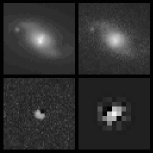
Figure 1.— Image subtraction as a solution to the problem of the contamination by complicated light distribution from the lensing galaxy. The two top panels are images of the QSO 2237+0305: reference image and typical test image (left and right respectively). The bottom panels show the corresponding difference image on the left and the best fit PSF matching kernel on the right. Note that the galaxy is completely removed by subtraction and the variable part of the flux is well modeled by the sum of the four PSF components at known positions. North is up and east is to the left.

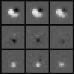
Figure 2.— Sample of nine difference images of the QSO 2237+0305 at various epochs from the OGLE data. North is up and east is to the left.

Figure 3.— Light curve of the QSO 2237+0305. Also shown is the light curve of the 18.14 mag reference star shifted by 1.1 mag for clarity. The polynomial fits help to assign the photometric points to each of the components.

Figure 4.— Same as Fig. 3 in mJy. Please note that the amplitudes of microlensing events in this linear plot are free of uncertainties associated with the zero point. The flux of the reference star has been lowered by 0.165 mJy for clarity.

Table 1Photometry of the QSO 2237+0305.

Date	[JD]	FWHM				$V$	mag
UT		arc sec	$A$	err	$B$	err	$C$	err	$D$	err
97-08-04.344	664.849	1.3	17.127	0.013	17.829	0.023	18.310	0.036	18.754	0.057
97-08-04.353	664.858	1.3	17.148	0.013	17.797	0.022	18.313	0.035	18.752	0.054
97-08-04.358	664.863	1.3	17.117	0.013	17.874	0.024	18.364	0.037	18.701	0.054
97-08-05.284	665.789	1.2	17.143	0.012	17.865	0.022	18.339	0.034	18.737	0.049
97-08-05.289	665.794	1.3	17.131	0.012	17.825	0.021	18.351	0.034	18.705	0.048
97-08-05.294	665.799	1.2	17.127	0.012	17.840	0.022	18.363	0.035	18.731	0.050
97-08-06.302	666.808	1.2	17.156	0.012	17.827	0.020	18.274	0.031	18.803	0.051
97-08-06.307	666.813	1.3	17.152	0.012	17.840	0.022	18.325	0.034	18.698	0.049
97-08-06.312	666.818	1.2	17.154	0.012	17.829	0.021	18.322	0.033	18.705	0.049
97-08-07.314	667.819	1.2	17.158	0.012	17.825	0.021	18.324	0.033	18.712	0.049
97-08-07.318	667.824	1.3	17.130	0.012	17.802	0.021	18.357	0.034	18.862	0.056
97-08-08.293	668.799	1.3	17.150	0.011	17.871	0.021	18.297	0.031	18.721	0.047
97-08-08.299	668.804	1.3	17.166	0.012	17.810	0.020	18.347	0.033	18.638	0.043
97-08-08.304	668.810	1.3	17.166	0.011	17.849	0.021	18.318	0.032	18.731	0.047
97-08-11.279	671.785	1.2	17.159	0.012	17.814	0.020	18.331	0.033	18.699	0.046
97-08-11.284	671.790	1.3	17.166	0.012	17.810	0.020	18.330	0.033	18.673	0.045
97-08-11.290	671.796	1.3	17.155	0.012	17.827	0.021	18.306	0.033	18.734	0.049
97-08-12.288	672.794	1.2	17.163	0.012	17.860	0.022	18.338	0.034	18.754	0.050
97-08-12.294	672.800	1.3	17.174	0.012	17.835	0.021	18.356	0.034	18.758	0.050
97-08-12.299	672.805	1.3	17.152	0.012	17.835	0.021	18.300	0.033	18.780	0.052
97-08-13.199	673.704	1.3	17.181	0.014	17.852	0.023	18.356	0.037	18.827	0.060
97-08-13.203	673.709	1.4	17.169	0.014	17.849	0.025	18.299	0.037	18.833	0.065
97-08-24.210	684.716	1.3	17.201	0.013	17.899	0.024	18.359	0.036	18.782	0.056
97-08-25.211	685.717	1.2	17.197	0.012	17.812	0.020	18.389	0.034	18.655	0.045
97-08-25.216	685.722	1.2	17.191	0.012	17.811	0.021	18.333	0.033	18.647	0.045
97-08-25.220	685.726	1.2	17.177	0.012	17.852	0.022	18.361	0.034	18.722	0.049
97-08-26.251	686.757	1.2	17.215	0.013	17.793	0.021	18.346	0.035	18.716	0.051
97-08-26.256	686.762	1.3	17.211	0.013	17.833	0.022	18.352	0.035	18.748	0.052
97-08-26.261	686.767	1.3	17.197	0.014	17.811	0.022	18.339	0.036	18.747	0.055
97-08-27.244	687.750	1.4	17.205	0.014	17.799	0.023	18.327	0.036	18.697	0.054
97-08-27.248	687.754	1.3	17.209	0.013	17.811	0.022	18.330	0.035	18.733	0.052
97-08-27.253	687.759	1.2	17.183	0.013	17.829	0.022	18.360	0.036	18.734	0.053
97-08-28.202	688.708	1.3	17.192	0.013	17.828	0.022	18.366	0.035	18.671	0.048
97-08-28.207	688.713	1.2	17.206	0.013	17.826	0.021	18.318	0.034	18.735	0.050
97-08-29.191	689.697	1.3	17.199	0.014	17.832	0.023	18.338	0.038	18.676	0.053
97-08-29.196	689.702	1.3	17.193	0.013	17.829	0.022	18.384	0.037	18.661	0.049
97-08-29.202	689.708	1.2	17.189	0.013	17.829	0.022	18.369	0.036	18.694	0.050
97-09-08.160	699.666	1.3	17.230	0.014	17.810	0.023	18.306	0.035	18.751	0.055
97-09-08.165	699.671	1.3	17.214	0.013	17.826	0.022	18.289	0.034	18.767	0.055
97-09-08.170	699.676	1.4	17.229	0.014	17.830	0.022	18.355	0.036	18.684	0.051
97-09-10.140	701.646	1.3	17.241	0.014	17.851	0.023	18.372	0.037	18.709	0.053
97-09-10.146	701.652	1.3	17.264	0.015	17.848	0.024	18.365	0.037	18.619	0.050
97-09-21.165	712.671	1.3	17.275	0.014	17.829	0.023	18.327	0.036	18.816	0.058
97-09-21.173	712.678	1.4	17.262	0.014	17.834	0.023	18.325	0.035	18.690	0.051
97-09-22.173	713.679	1.3	17.257	0.014	17.843	0.023	18.335	0.036	18.781	0.057
97-09-22.179	713.685	1.2	17.276	0.015	17.858	0.023	18.333	0.036	18.785	0.056
97-09-23.183	714.689	1.2	17.276	0.013	17.859	0.022	18.373	0.035	18.798	0.052
97-09-23.189	714.695	1.2	17.284	0.014	17.861	0.022	18.363	0.035	18.788	0.052
97-09-24.178	715.684	1.3	17.255	0.014	17.855	0.022	18.357	0.035	18.752	0.052
97-09-24.183	715.689	1.2	17.258	0.014	17.836	0.022	18.368	0.037	18.725	0.052
97-10-06.124	727.629	1.3	17.271	0.015	17.848	0.023	18.314	0.035	18.678	0.051
97-10-06.132	727.637	1.3	17.288	0.014	17.838	0.022	18.336	0.035	18.691	0.051
97-10-07.238	728.744	1.3	17.335	0.016	17.916	0.025	18.344	0.038	19.025	0.074
97-10-07.248	728.753	1.3	17.325	0.016	17.909	0.025	18.417	0.039	19.010	0.071
97-10-09.203	730.708	1.3	17.288	0.016	17.782	0.023	18.273	0.035	18.727	0.057
97-10-09.208	730.713	1.3	17.311	0.017	17.808	0.024	18.242	0.036	18.736	0.062
97-10-20.097	741.601	1.3	17.285	0.015	17.817	0.022	18.297	0.034	18.792	0.057
97-10-20.101	741.605	1.2	17.300	0.014	17.828	0.022	18.342	0.035	18.850	0.057
97-10-21.118	742.622	1.3	17.310	0.015	17.781	0.021	18.272	0.033	18.745	0.053
97-10-21.122	742.626	1.2	17.298	0.014	17.803	0.021	18.270	0.032	18.814	0.055
97-10-24.119	745.623	1.2	17.299	0.014	17.805	0.021	18.276	0.032	18.695	0.049
97-10-24.123	745.627	1.2	17.310	0.014	17.792	0.021	18.332	0.034	18.804	0.053
97-10-25.131	746.635	1.2	17.308	0.015	17.796	0.022	18.237	0.033	18.825	0.058
97-10-25.135	746.639	1.3	17.306	0.014	17.782	0.021	18.279	0.033	18.852	0.058
97-10-31.058	752.562	1.2	17.285	0.014	17.773	0.021	18.283	0.033	18.780	0.053
97-10-31.062	752.566	1.2	17.298	0.014	17.808	0.021	18.302	0.033	18.793	0.053
97-11-01.040	753.544	1.2	17.303	0.014	17.777	0.021	18.252	0.032	18.777	0.053
97-11-01.044	753.548	1.4	17.304	0.014	17.796	0.021	18.289	0.033	18.852	0.056
97-11-18.086	770.588	1.3	17.311	0.014	17.791	0.021	18.278	0.033	18.823	0.055
97-11-18.090	770.592	1.3	17.351	0.015	17.832	0.022	18.235	0.032	18.828	0.056
97-11-21.087	773.589	1.3	17.314	0.015	17.781	0.022	18.251	0.033	18.785	0.057
97-11-21.091	773.593	1.2	17.341	0.016	17.769	0.022	18.238	0.033	18.798	0.058
97-11-27.094	779.595	1.4	17.324	0.017	17.763	0.023	18.256	0.035	18.760	0.061
97-11-27.098	779.599	1.3	17.353	0.020	17.791	0.027	18.274	0.040	18.696	0.069
97-11-29.039	781.540	1.3	17.332	0.015	17.777	0.021	18.251	0.033	18.769	0.055
97-11-29.043	781.544	1.3	17.339	0.015	17.803	0.022	18.274	0.034	18.761	0.056
97-12-02.053	784.554	1.3	17.328	0.015	17.774	0.022	18.200	0.032	18.680	0.052
97-12-02.057	784.558	1.3	17.311	0.015	17.799	0.022	18.244	0.033	18.830	0.058
97-12-17.035	799.534	1.3	17.354	0.018	17.811	0.025	18.234	0.036	18.856	0.072
97-12-17.040	799.539	1.3	17.346	0.017	17.827	0.024	18.218	0.034	18.901	0.069
98-08-16.168	1041.674	1.2	17.142	0.013	18.103	0.029	17.595	0.019	18.406	0.041
98-08-16.174	1041.680	1.3	17.120	0.013	18.089	0.028	17.591	0.018	18.436	0.041
98-08-29.224	1054.730	1.3	17.143	0.012	18.089	0.026	17.538	0.017	18.420	0.037
98-08-29.228	1054.734	1.3	17.136	0.012	18.125	0.027	17.578	0.017	18.429	0.038
98-08-29.237	1054.743	1.4	17.131	0.012	18.108	0.027	17.568	0.017	18.371	0.036
98-08-29.241	1054.747	1.3	17.156	0.012	18.120	0.027	17.579	0.017	18.389	0.036
98-11-08.069	1125.572	1.2	17.110	0.011	18.194	0.029	17.579	0.017	18.308	0.033
98-12-15.039	1162.539	1.3	17.192	0.013	18.177	0.030	17.645	0.019	18.206	0.032
98-12-15.047	1162.546	1.2	17.160	0.012	18.229	0.030	17.667	0.018	18.340	0.035
98-12-15.051	1162.550	1.2	17.166	0.012	18.195	0.029	17.640	0.018	18.311	0.034
98-12-15.057	1162.556	1.2	17.178	0.012	18.228	0.030	17.659	0.018	18.250	0.032
98-12-15.061	1162.560	1.2	17.155	0.012	18.175	0.028	17.630	0.018	18.272	0.032
98-12-17.037	1164.536	1.3	17.150	0.013	18.173	0.031	17.643	0.019	18.284	0.037
98-12-17.041	1164.540	1.3	17.178	0.014	18.221	0.033	17.665	0.020	18.304	0.039
98-12-18.029	1165.528	1.3	17.137	0.013	18.267	0.034	17.679	0.020	18.357	0.039
98-12-18.033	1165.532	1.3	17.176	0.013	18.249	0.032	17.641	0.019	18.277	0.035
98-12-18.043	1165.542	1.4	17.163	0.013	18.183	0.031	17.688	0.020	18.382	0.040
98-12-18.047	1165.546	1.4	17.151	0.014	18.257	0.034	17.630	0.020	18.367	0.041
98-12-19.033	1166.532	1.3	17.178	0.015	18.229	0.036	17.598	0.021	18.364	0.046