The Properties of Field Elliptical Galaxies at Intermediate Redshift. I: Empirical Scaling Laws

Abstract

We present measurements of the Fundamental Plane (FP) parameters (the effective radius, the mean effective surface brightness, and the central velocity dispersion) of six field elliptical galaxies at intermediate redshift. The imaging is taken from the Medium Deep Survey of the Hubble Space Telescope, while the kinematical data are obtained from long-slit spectroscopy using the 3.6-m ESO telescope. The Fundamental Plane appears well defined in the field even at redshift $\approx$ 0.3. The data show a shift in the FP zero point with respect to the local relation, possibly indicating modest evolution, consistent with the result found for intermediate redshift cluster samples. The FP slopes derived for our field data, plus other cluster ellipticals at intermediate redshift taken from the literature, differ from the local ones, but are still consistent with the interpretation of the FP as a result of homology, of the virial theorem and of the existence of a relation between luminosity and mass, $L\propto M^{\eta}$. We also derive the surface brightness vs. effective radius relation for nine galaxies with redshift up to $z\approx 0.6$, and data from the literature; the evolution that can be inferred is consistent with what is found using the FP.

1 Introduction

Elliptical galaxies in the local universe are known to populate only a two-dimensional manifold, known as the Fundamental Plane (hereafter FP; Djorgovski & Davis 1987; Dressler et al. 1987), in the three-dimensional space defined by effective radius $R_{\textrm{e}}$, mean surface brightness within the effective radius SB${}_{\textrm{e}}$ (SB${}_{\textrm{e}}=-2.5\log\langle I\rangle_{\textrm{e}}+$const; I is the surface brightness in linear flux), and central velocity dispersion $\sigma$. The FP is described by:

$$\log R_{\textrm{e}}=\alpha\log~{}\sigma+\beta~{}\textrm{SB}_{\textrm{e}}+\gamma,$$ (1)

$R_{\textrm{e}}$ is in kpc (while $r_{\textrm{e}}$ is in arcsecs), $\sigma$ in km $\textrm{s}^{-1}$, SB${}_{\textrm{e}}$ in $\textrm{mag arcsec}^{-2}$ and $H_{0}$ is hereafter assumed to be 50 $h_{50}$ km $\textrm{s}^{-1}$$\textrm{Mpc}^{-1}$. Typical values of the coefficients are for example $\alpha=1.25$, $\beta=0.32$ and $\gamma=-8.895$ in Johnson B (Bender et al. 1998; hereafter B98). It is still unclear whether the thickness of the FP is intrinsic, i.e., due to scatter in the properties of elliptical galaxies, or is due to observational errors.

The existence of the empirical scaling described by the FP has strong implications in terms of galactic evolution and formation theories. For example, the FP suggests that the distributions of dark and luminous matter are related, since $\sigma$ depends on the total gravitational potential, whereas SB${}_{\textrm{e}}$ and $R_{\textrm{e}}$ trace only the stellar mass. The FP can be explained in terms of homology, of the virial theorem, and of the existence of a well-defined relation between luminosity and mass, $L\propto M^{\eta}$ (Faber et al., 1987; see also van Albada, Bertin & Stiavelli 1995). This interpretation requires a relation between the derived values of $\alpha$ and $\beta$, namely $\alpha-10\beta+2=0$ ($\eta=0.2~{}\alpha/\beta$).

Measuring the FP parameters for ellipticals at intermediate redshift $z\approx 0.3$–$0.8$ has only recently become feasible (Pahre, Djorgovski & de Carvalho 1995; van Dokkum & Franx 1996; Bender et al. 1996; Kelson et al. 1997; van Dokkum et al. 1998). This opens up two important questions which bear on the age, formation history, and internal properties of elliptical galaxies: i) how far in the past does an FP-like relation apply? and ii) do its parameters evolve significantly with time? The existence of a tight FP-like relation at substantial look-back times would suggest the existence of a universal relation between mass and formation time for ellipticals, since, e.g., population differences would be amplified as the redshift increases. Existing measurements of the properties of ellipticals at intermediate redshifts have concentrated so far on relatively rich clusters of galaxies, where bright ellipticals are easier to find [Pahre et al. 1995, van Dokkum & Franx 1996, Bender et al. 1996, Ziegler & Bender 1997, Kelson et al. 1997, van Dokkum et al. 1998] and observations can be carried out efficiently with multi-object spectrographs. When comparing, e.g., the FP of intermediate redshift and zero redshift clusters one must take into account the evolution with redshift of the population of galaxies in clusters, and environmental effects. Although the evolution of clusters of galaxies is still somewhat controversial [Postman et al. 1996], the galaxy population in rich clusters is likely to become less uniform (in terms, e.g., of age and metallicity) with time, due to accretion of isolated galaxies and small groups. Moreover, the question of whether there are systematic differences between cluster and field ellipticals (the latter including galaxies in loose groups or poor clusters) is still open even at low redshift [de Carvalho & Djorgovski 1992]. A study of the galaxy properties as a function of look-back time provides a sensitive probe of the possible evolutionary differences between cluster and field ellipticals. For these reasons, we have begun a study of the empirical scaling laws of field ellipticals at intermediate redshift.

We have started out by defining a sample of ellipticals which is not biased in favour of rich clusters. Details on the selection process are given in Section 2. Sections 3 and 4 describe the data reduction and the error analysis. Measurements at non-zero redshift have to be carried out with photometric filters and effective apertures that differ from those used to derive the local scaling laws; Section 5 describes the conversion of our measurements to the standard quantities. The main results are reported in Section 6, where our measurements are compared to local samples and intermediate redshift cluster samples. A summary is given in Section 7.

2 Sample selection

With this study we aim at addressing two questions: i) does the FP of field ellipticals evolve with redshift? and ii) do, at any given redshift, the field ellipticals have FP parameters different from those found in rich cluster environments? For this we need to select a primary sample of galaxies biased against rich cluster membership at intermediate redshift, where the project is feasible and the look-back time ($\approx 4$–$5$ Gyrs) is high enough that evolution can be noticeable.

The targets used in this study have been chosen among a sample of random ellipticals found in the WFPC2 parallel images collected by the Medium Deep Survey [Griffiths et al. 1994]. The target pool has been selected originally from available HST images in the appropriate RA, $\delta$ range according to the following criteria:

1. Apparent magnitude $I<20.5$

2. Morphology clearly defined as elliptical, with an apparent effective radius $r_{\textrm{e}}>0\aas@@fstack{\prime\prime}5$.

3. $V-I$ colour in agreement with the empiric relation for ellipticals in the redshift range $0.2\leq z\leq 0.5$ ($1.1<V-I<1.7$)

Magnitudes and colours above are as defined by the Medium Deep Survey group [Griffiths et al. 1994]; $V$ and $I$ are the magnitudes in the WFPC2 filters F606W and F814W, computed in the WFPC2 Flight system (Holtzman et al. 1995), and the effective radius $r_{\textrm{e}}$ is the value found from the two-dimensional image fitting carried out by the MDS. All photometric parameters have been rederived here with two different techniques (see Section 3) to ensure a self-consistent treatment.

Individual targets were then selected from this pool of approximately 25 candidates on the basis of convenience and availability during each observing night; in the spirit of this exploratory study, we did not attempt further to achieve uniformity or completeness within our pool of candidates.

Since we did not explicitly exclude members of poor clusters (no rich clusters were observed in these random fields), the ellipticals in our sample should be representative of a random, magnitude-selected sample of non-rich-cluster objects. In fact, four of the six objects for which we have obtained FP parameters happen to be members of a group (or a poor cluster), which was randomly observed in the available HST images. Future observations will enable us to achieve a better level of completeness and thus to better characterise our sample.

Our colour selection criterion will bias against actively star-forming ellipticals, which are known to occur, albeit infrequently, in complete samples [Lilly et al. 1995]. We plan to relax the blue cutoff in future observations.

2.1 Target list

The characteristics of the objects we observed are summarised in Table 1. The final sample used in the discussion in Section 6 is composed of the galaxies successfully fitted with the two different photometric techniques, isophotal profile fit and two-dimensional fit, and with measured kinematics.

The photometry of C, L, M, N was of low quality due to companion galaxies, stars in the field of view and the faintness of the objects. The 2D fit was performed only on the galaxies with a high quality isophotal profile. We were able to determine high quality photometric parameters for G by subtracting a model of its companion H from the image before the 2D fit.

Table 1: Galaxy identification. (1) Adopted names, (2) HST Medium Deep Survey field name, (3) WFPC2 chip, (4) ID within the field, (5) and (6) pixel positions of the center of the galaxy, (7) Sizes of the F606W and F814W images used in the 2D fits and displayed in Figures 2 and 3. The image used for I in F814W was $5\aas@@fstack{\prime\prime}4\times 4\aas@@fstack{\prime\prime}8$. Dashes in Column 7 indicate that the 2D fit was not performed.

galaxy	field	chip	n	x	y	size
(1)	(2)	(3)	(4)	(5)	(6)	(7)
A	ut800	4	1	324	444	$18^{\prime\prime}\times 18^{\prime\prime}$
B	ut800	4	2	265	741	$8^{\prime\prime}\times 8^{\prime\prime}$
C	ur610	3	1	678	691	-
D	ur610	3	2	723	642	$9\aas@@fstack{\prime\prime}5\times 6\aas@@fstack{\prime\prime}4$
E	u5405	2	1	335	324	$8^{\prime\prime}\times 7^{\prime\prime}$
F	u5405	2	2	332	221	$5\aas@@fstack{\prime\prime}4\times 6\aas@@fstack{\prime\prime}4$
G	u5405	2	3	192	288	$10^{\prime\prime}\times 10^{\prime\prime}$
H	u5405	2	4	194	255	-
I	u5405	2	5	72	63	$5\aas@@fstack{\prime\prime}2\times 4\aas@@fstack{\prime\prime}3$
L	u5405	3	6	254	711	-
M	u5405	3	7	266	715	-
N	u5405	3	8	747	732	-
O	ust00	3	1	226	523	$5^{\prime\prime}\times 5^{\prime\prime}$
P	ust00	3	2	336	404	$5^{\prime\prime}\times 5^{\prime\prime}$
Q	ust00	3	3	443	298	$5\aas@@fstack{\prime\prime}2\times 5\aas@@fstack{\prime\prime}4$
R	urz00	2	1	719	242	-

3 Photometry

The images are taken from the Medium Deep Survey of the Hubble Space Telescope [Griffiths et al. 1994]. For each field there are images from WFPC2 through filters F606W and F814W. Table 2 lists total exposure times and number of exposures.

Table 2: Photometric data: number of exposures (nexp) and total exposure times (texp).

field	filter	nexp	texp (s)
u5405	F606W	1	800
	F814W	1	800
ur610	F606W	2	1500
	F814W	2	1600
urz00	F606W	3	5400
	F814W	4	8400
ust00	F606W	10	16500
	F814W	11	23100
ut800	F606W	2	1430
	F814W	3	4430

3.1 Reduction

The basic reduction was done at the Space Telescope Science Institute using the standard pipeline with the best reference files available. As bias and dark files we used the superbias and the superdark from the Hubble Deep Field [Williams et al. 1996] for their high signal-to-noise ratio. The cosmic ray removal for the fields with multiple images was done using the iraf/stsdas task crrej, with a cutoff at 5 standard deviations from the mean. Since only one exposure per filter was available for u5405, the original image of this field was compared with a smoothed version (using the midas command filter/cosmic). In all cases we checked by eye that the pixels removed in the area of the targets were only those affected by cosmic rays.

For u5405, chip 2 of WFPC2 is affected by a bad column, very close to the center of galaxies E and F (see Figure 2). We interpolated through it in the outer parts of the galaxies, but we chose not to modify the 4-5 pixel diameter central zone because it was too steep for any interpolation to be meaningful (see also Figure 1). In order to test how much this bad column affected the determination of the photometric parameters, we fitted the isophotal profile of E excluding the innermost part of the profile. We tried excluding a 2 pixel and a 4 pixel diameter circle; the effective radius and the effective surface brightness change significantly (up to 20% in $r_{\textrm{e}}$), towards the value given by the 2D fit (smaller $r_{\textrm{e}}$ and brighter surface brightness). These new values are still consistent with the average value within the internal errors (that are the largest of the sample, see Subsection 3.4). Furthermore it should be noticed that the derived values for $r_{\textrm{e}}$ and SB${}_{\textrm{e}}$ are highly correlated and therefore the variation of the combination that enters the FP, $\log r_{\textrm{e}}-\beta\textrm{SB}_{\textrm{e}}$, is much smaller than the variation on the single coefficients (see Subsection 3.4 and Table 5).

A constant sky contribution was subtracted from each image. The sky contribution used was the mean of the averages of areas with no evidence for light sources. This procedure does not take into account smooth and diffuse background sources, which is one of the main sources of uncertainty when using curve of growth technique (see Section 3.4).

3.2 Isophotes and two-dimensional fits

The photometric parameters needed for the FP are the effective radius $r_{\textrm{e}}$, and the effective surface brightness SB${}_{\textrm{e}}$, measured as the best $r^{1/4}\,$light profiles parameters.

In order to obtain the best results and robust error estimates, the photometric parameters were derived using two independent techniques: fits to the isophotal luminosity profiles and two-dimensional fits to the images. Both procedures require a PSF to convolve the models with. We used synthetic PSFs calculated with Tiny Tim 4.0 [Krist 1994] with a 15 mas jitter. The quality of the synthetic PSF was checked by comparing the isophotal profiles of two stars and the profiles of two PSFs created in the same spot. No significant difference was noticed. As a double-check we fitted an isophotal profile using both a synthetic PSF profile and a real star profile: the differences were less than 1% in $r_{\textrm{e}}$ and less than 0.02 mag in SB${}_{\textrm{e}}$. The photometric parameters of each galaxy were derived independently in the two bandpasses F814W and F606W.

3.2.1 Isophotes

Isophotes were fitted to the images with the center of the ellipse, the semiaxes $a$ and $b$, and the position angle as free parameters; variations of ellipticity ($e$) and position angle ($pa$) with the “circularised” radius $\sqrt{ab}$ were allowed. Isophotes were derived using a version of the midas command fit/ell3 modified to better deal with steep gradients in the luminosity profile in the innermost pixels (Møller, Stiavelli & Zeilinger, 1995). The profiles obtained were fitted with an exponential law, an $r^{1/4}\,$law, and a linear combination of the two. In all cases, except for B, we found that the objects were best fitted by the $r^{1/4}$ law. A slightly better fit of the light profile of galaxy B was obtained by adding a small exponential component to the $r^{1/4}\,$law, suggesting that the bump on the residual might be due to a fainter disk component (see Figures 1 and 3). The fit was done using the least squares fitting software used by Carollo et al. [Carollo et al. 1997]. For each galaxy we used a specific PSF calculated at its position. In Figure 1 we show the best-fit $r^{1/4}\,$laws convolved with the PSFs, superimposed on the data points.

Figure 1: Isophotal profiles. Crosses are the data points, solid lines represent the best-fit $r^{1/4}\,$profile, convolved with the PSF. The upper data refer to F814W, the lower to F606W. The error bars (which are smaller than the crosses for the innermost part of the profile) take into account the sky-subtraction error. The bump on the B profile is possibly the signature of a disk component (see text, Section 3.2.1, and the two dimensional residual in Figure 3). The central surface brightness decline in E is likely to be caused by the bad column right at the center of the galaxy.

3.2.2 Two-dimensional fits

This technique consists in fitting a two-dimensional model of an elliptical galaxy, as seen on the CCD chip, to the WFPC2 image. The model galaxy has an $r^{1/4}\,$luminosity profile, with fixed position angle and ellipticity (we used the value derived from the isophotal fit near the effective radius). Each fit has four free parameters: the effective surface brightness, the effective radius, and the position of the centre. We have two sets of results, depending on how the fit was performed (see (iv) below). The software we developed works as follows:

1. The code generates a 2D projected image of the galaxy using the $r^{1/4}\,$law on a subsampled grid. The pixel size is chosen to be approximately ten times smaller than the galaxy effective radius in order to make discretisation problems negligible.

2. The resulting “ideal” model is rebinned to the WFPC2 chip scale.

3. The rebinned model is convolved with the Tiny Tim [Krist 1994] PSF. The Tiny Tim (non resampled) PSF includes the effects of diffraction (i.e. of the telescope and camera optics) and the Pixel Response Function (i.e. the spread caused by electron diffusion in the WFPC2 CCDs).

4. This model is fitted to the data either by least $\chi^{2}$ or by least squares, using a simplex algorithm to find the minimum (amoeba, Press et al. 1992).

For each galaxy we ran the code twice, minimising both the $\chi^{2}$ and the unweighted residuals (least squares). In the case of G the fit was not straightforward because of the companion H. Therefore we subtracted from the data, before performing the fit, a model for H, obtained from an $r^{1/4}\,$profile with $r_{\textrm{e}}$, SB${}_{\textrm{e}}$, $pa$, and $e$ taken from the isophotal profile fit. The result was stable with respect to variations of the parameters of H. In Figure 2 and 3 the original WFPC2 image and the fit residual are shown for all the galaxies fitted with the 2D fits.

A

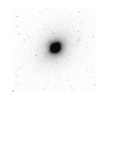
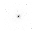
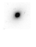
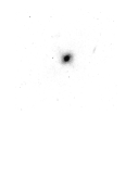
D

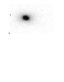
E

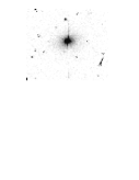
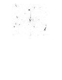
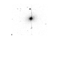
F

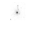
GH

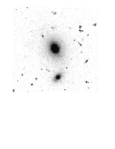
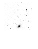
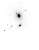
I

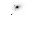
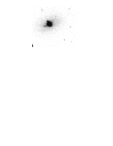
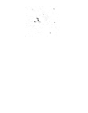
Figure 2: WFPC2 images and 2D fit residuals for the galaxies with measured kinematics: A,D, E, F, G, I. From the left to the right we display the F606W image, the F606W residual, the F814W image and the F814W residual. The images (and their sizes) are the ones used for the 2D fits, see Table 1. Galaxies A, D show a residual in the innermost pixels which is in agreement with the deviation from the $r^{1/4}\,$law in the luminosity profile. The bad column in the centre of E is clearly evident in the residual. F shows a peculiar pot handle structure just to the upper left of the bad column.

B

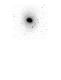
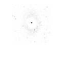
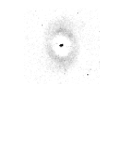
O

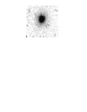
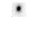
P

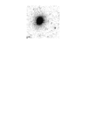
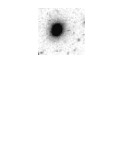
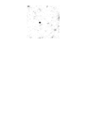
Q

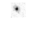
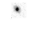
Figure 3: WFPC2 images and 2D fit residuals for the galaxies without measured kinematics: B,O,P,Q. In the residual of B a spiral pattern is recognizable.

3.2.3 Results

All galaxies are well fitted by the $r^{1/4}\,$law (de Vaucouleurs 1948) with the exception of galaxy B which shows face-on spiral-like residuals and might be an early-type spiral.

Figure 4: Comparison of photometric parameters from the isophotal profile fit (x-axis) with those from one of the 2D fits (the least $\chi^{2}$, y-axis). Subscripts 6 and 8 indicate filters F606W and F814W.

Standard magnitudes are obtained from the data following the Holtzman et al. [Holtzman et al. 1995] calibration. In Figure 4 we plot the photometric parameters obtained from one of the 2D fits (the least $\chi^{2}$) versus those given by the isophotal profile fit. The results are in very good mutual agreement, even though the procedures differ in some important details, e.g., the isophotal profile fit is in magnitudes and allows for $pa$ and $e$ variation, while the 2D fits are in counts and have fixed $pa$ and $e$. As final value of the parameters we use the average of the three results; the photometric parameters are shown in Tables 3 and 4. Integrated luminosities are those of the best-fitting $r^{1/4}$ law.

Table 3: Photometric parameters through filter F606W. Errors (see Section 3.4) do not include sky-subtraction contributions, which we estimate to be 0.5 per cent on $r_{\textrm{e}}$, 0.05 mag $\textrm{arcsec}^{-2}$ on SB${}_{\textrm{e}}$ and 0.02 mag on m (see text for details).

galaxy	$r_{\textrm{e}}$	$\delta r_{\textrm{e}}$	SB${}_{\textrm{e}}$	$\delta\textrm{SB}_{\textrm{e}}$	m	$\delta\textrm{m}$
A	1.65	0.13	20.64	0.13	17.57	0.12
B	0.588	0.038	19.73	0.11	18.90	0.05
D	0.793	0.042	20.99	0.09	19.5	0.03
E	0.794	0.071	21.60	0.13	20.12	0.06
F	1.145	0.017	22.56	$<0.01$	20.27	0.03
G	1.589	0.064	21.81	0.07	18.81	0.01
I	0.636	0.046	20.92	0.13	19.92	0.04
O	0.795	0.011	23.15	0.05	21.65	0.02
P	0.526	0.029	22.20	0.11	21.66	0.01
Q	0.612	0.018	23.20	0.06	22.27	0.02

Table 4: Photometric parameters through filter F814W (same as Table 2).

galaxy	$r_{\textrm{e}}$	$\delta r_{\textrm{e}}$	SB${}_{\textrm{e}}$	$\delta\textrm{SB}_{\textrm{e}}$	m	$\delta\textrm{m}$
A	1.99	0.15	19.92	0.19	16.44	0.13
B	0.548	0.014	18.58	0.05	17.89	0.04
D	0.645	0.058	19.29	0.16	18.27	0.04
E	0.872	0.080	20.31	0.12	18.64	0.07
F	1.29	0.12	21.33	0.11	18.81	0.10
G	1.419	0.075	20.29	0.09	17.53	0.02
I	0.606	0.051	19.47	0.15	18.58	0.03
O	0.654	0.007	21.02	0.05	19.94	0.02
P	0.502	0.018	20.48	0.08	19.98	$<0.01$
Q	0.547	0.053	21.14	0.17	20.48	0.03

3.3 A cross-check with the growth curve technique

The growth curve technique is a standard procedure for nearby samples. Two problems of this technique are: i) the statistical dependence between different aperture magnitudes, e.g. in the presence of light coming from a nearby galaxy or of diffuse background sources, the systematic error affects the flux within all the apertures; ii) the sensitivity to sky-subtraction errors. We measured the photometric parameters by fitting the growth curve of an $r^{1/4}$ profile to the aperture magnitudes and the results were in reasonably good agreement with the other two methods.

3.4 Error analysis

We define as internal error of the parameters the standard deviation of the results of the two 2D fits and the isophotal profile fit. Since photon shot noise is negligible in our context, the main source of error not included in the internal error is the uncertainty due to sky subtraction (0.5 per cent on $r_{\textrm{e}}$, 0.02 mag on m, 0.05 mag $\textrm{arcsec}^{-2}$ on SB${}_{\textrm{e}}$). We estimated this uncertainty by measuring how the photometric parameters changed with the sky level, and we added it quadratically to the internal error, so as to obtain the total error; more precisely we used the variation of the photometric parameters when the sky is shifted by one standard deviation, calculated as the scatter of the sky levels measured in different areas (a typical value is 2%). The photometric parameters $r_{\textrm{e}}$ and $\langle I\rangle_{\textrm{ e}}$ are correlated, as can be seen from the errors calculated directly and reported in Table 5. The particular combinations of effective radius and surface brightness are chosen because they enter the definition of the $\kappa$ space (Bender, Burstein & Faber 1992). Also the error on the colour ($m_{\textrm{\small F606W}}-m_{\textrm{\small F814W}}$) is different from the sum of errors on the single filter magnitudes (see Table 5) since the errors in the two filters are correlated: it generally happens that when one method (e.g. 2D $\chi^{2}$) gives a lower magnitude than another (e.g. profile fits), the same thing is repeated in both filters.

Table 5: Photometric parameters II. Errors are shown as examples of the correlation of the photometric uncertainties. The quantity $colour$ is defined as $m_{\textrm{\small F606W}}-m_{\textrm{\small F814W}}$.

galaxy	colour	$\delta$colour	$\delta\langle I\rangle_{\textrm{e}}^{2}r_{\textrm{e}}^{-1}/\langle I\rangle_{\textrm{e}}^{2}r_{\textrm{e}}^{-1}$	$\delta\langle I\rangle_{\textrm{e}}r_{\textrm{e}}/\langle I\rangle_{\textrm{e}}r_{\textrm{e}}$
A	1.127	0.012	0.23	0.089
B	1.015	0.012	0.24	0.047
D	1.226	0.018	0.19	0.027
E	1.486	0.013	0.29	0.034
F	1.463	0.068	0.025	0.011
G	1.273	0.007	0.15	0.028
I	1.333	0.005	0.28	0.044
O	1.705	0.006	0.091	0.028
P	1.678	0.013	0.26	0.045
Q	1.789	0.051	0.15	0.031

4 Spectroscopy

The spectroscopic observing run took place in the period April 18-22 1996 at the 3.6-m ESO telescope. Long slit ($1\aas@@fstack{\prime\prime}5$ slit width) spectroscopy was obtained with the EFOSC spectrograph, with the Orange 150 grism in the spectral range between approximately 5200 and 7000 Å  (512$\times$512 CCD, with pixel size 30 $\mu m$ equivalent to about $0\aas@@fstack{\prime\prime}57$). The slit length of about $180\arcsec$ projects to only about 320 pixels on the CCD. For each target we obtained multiple exposures. The estimated seeing, measured with R-band acquisition images, was $0\aas@@fstack{\prime\prime}8$ FWHM. Table 6 gives the basic observation log.

Table 6: Spectroscopic data: number of observations (nexp), total exposures times (texp), and average signal-to-noise ratio per pixel (S/N).

galaxy	nexp	texp (s)	S/N
A	4	7200	65
B	4	7200	40
D	4	12000	22
E	5	13200	17
F	5	13200	12
G	3	10800	35
I	3	10800	22
LM	2	4800	-
N	2	4800	-
O	10	36000	7
P	10	36000	6
Q	10	36000	-

The slit positions were carefully chosen to include as many objects (two or three at a time) as possible. Every night we obtained an exposure with the He-Ar lamp at zenith; before and after every galaxy spectrum we took a He lamp spectrum as a check of the dispersion relation shifts. We observed two spectrophotometric standard white dwarfs in order to perform relative-flux calibration of the spectra. The identification of our targets as normal, non star-forming, ellipticals was confirmed by the absence of emission lines in their spectra.

4.1 Reduction

A superbias file was obtained by averaging about a hundred bias images and was subtracted from the data. Dome flatfield exposures were used to produce a flatfield along the wavelength direction (CCD columns). The slit function was obtained from sky frames and was found to be independent of wavelength. Dark current subtraction was done by producing a dark frame from the average of 8 darks 1 hour long. Since this mean dark did not contain structures, we only subtracted the mean value.

Throughout the reduction and analysis we have avoided (non-linear) rebinnings. To this end, we did the reduction before wavelength calibration. The extraction of the spectra was a crucial point of the reduction process, given the faintness of the signals. Averaging too many rows would have meant too much noise, using only the central row would have meant losing important signal. As we could not simply extract a fixed pixel width (along the spatial direction) because of optical distorsions, we used a code developed by Møller & Kjærgaard (1992) to obtain a one-dimensional spectrum, extracted with optimal signal-to-noise weighting. The code also removes cosmic rays, identified as pixels five standard deviations away from the expected signal. All spectra were carefully inspected by eye before and after extraction to check the proper cosmic ray removal.

Given the faint signal of the spectra, we took special care during sky subtraction. For each galaxy we extracted two sets of columns, to the left and to the right of the galaxy. The columns were selected to be as close as possible to the galaxy to limit optical distorsion problems. Columns of one set were combined neglecting the highest and lowest pixels to remove cosmic rays. The result was eye-inspected and then the two spectra obtained were averaged to obtain a high signal-to-noise sky spectrum. This procedure allowed us to check the optical distorsion by comparing the emission lines between the left and the right spectra. The sky spectra obtained had broader lines than the single column ones, because we combined spectra wavelength-shifted by optical distorsion. Sky contribution was subtracted during spectrum extraction by deconvolving the artificial additional width. The resulting one-dimensional spectra were combined to obtain the final galactic spectrum, after verifying that the relative shifts of the positions along the y-axis of the emission lines were negligible. The reduced spectra are shown in Figure 5. The average signal-to-noise ratio per pixel of the spectra is listed in Table 6. The average signal-to-noise ratio ranges from 65 per pixel for the brightest galaxy (A) to 12 per pixel for the faintest galaxy for which we obtained a velocity dispersion (F); the estimated error is accordingly larger for F than for A. For comparison, Davies et al. (1987) in their low redshift study, with a total signal-to-noise ratio equivalent to 5$\cdot 10^{5}$ photons, estimate the random error to be about 10 %. The analysis in Section 6 is done both with the entire sample and excluding the two galaxies E and F with the lowest signal-to-noise spectra among those with measured velocity dispersion.

4.2 Wavelength calibration and measurement of the instrumental resolution

We found the dispersion relation for each He-Ar lamp using the midas gui/long software. The different calibrations were all within the errors. We used short He lamp images to check that shifts between single exposures were negligible. The He-Ar lamps were also used to measure the instrumental resolution: the line shapes were fitted with Gaussian functions to obtain line widths as a function of CCD pixel number, and, via dispersion relation, of wavelength. The FWHM is independent of $\lambda$ within the measurement scatter and it was determined to be:

$$\Delta\lambda=(8.39\pm 0.26)\textrm{\AA},$$ (2)

Translated into velocities it corresponds to a kinematic resolution ranging from 206 to 155 km $\textrm{s}^{-1}$  from the blue to the red. The 3 % error is due to the scatter in the measurement (see also Section 4.4). The instrumental resolution measurement is very important for the kinematic fit, as we discuss in Section 4.3. Therefore we carefully examined all lines, to avoid ghost lines which were found and which would have affected the measurement. We checked the resolution by measuring the width of the sky lines and the results were consistent with the ones found with the He-Ar lamp (8.11$\pm$0.39 Å).

For comparison, the instrumental resolution of the Lick/IDS spectrograph was between 8-10 Å  at shorter wavelengths (see e.g. Dalle Ore et al., 1991). The velocity dispersions we find are larger than half the instrumental resolution, which is commonly considered as a limit (see e.g. Dressler 1979; Kormendy 1982; Bender, 1990). It has been noticed that when the velocity dispersion becomes of the order of the kinematic resolution and the signal-to-noise is low a systematic error may be introduced (see e.g. Jørgensen, Franx & Kjærgaard, 1995). In order to study this effect we broadened some stellar templates to 150, 200, 250, 300 km $\textrm{s}^{-1}$and we added noise, thus producing artificial galaxies with S/N per pixel ranging between 10 and 60. The artificial galaxies were then fitted with the same stellar templates to measure how well the original velocity dispersions were recovered. The largest velocity dispersions were recovered within few percents (2–4 %) down to S/N=10, while the smaller one (150 km $\textrm{s}^{-1}$) resulted systematically underestimated by $\sim 10$% at S/N 10. No systematic trends were noticed above S/N=15. This bias is negligible to our measurement, as galaxies E and I, the only with measured velocity dispersion below 200 km $\textrm{s}^{-1}$(see Table 7), have high enough S/N (see Table 6), while F, the only with S/N below 15 has $\sigma\approx 200$ km $\textrm{s}^{-1}$.

Figure 5: Wavelength (in Å) calibrated spectra of the galaxies with measured velocity dispersion. The shaded spectral regions were affected by strong sky-emission lines. These regions have not been used in the kinematic fit. The standard deviation per pixel is also shown (lower curves). The arrows identify some of the main absorption features, such as Ca H (3968.5 Å) and K (3933.7 Å), the G band (4304.4 Å), Mg_b (5175.4 Å) and Na D (5892.5 Å).

4.3 Kinematics

In order to derive a robust measurement of the kinematics of our sample of galaxies we used two different and independent codes: i) the Gauss-Hermite Fourier Fitting Software [Franx, Illingworth & Heckman 1989, van der Marel & Franx 1993], hereafter GHFF, and ii) the Fourier Quotient [Sargent et al. 1977], hereafter FQ, in the version modified by Rose (Dressler, 1979) and used e.g. by Stiavelli, Møller & Zeilinger (1993). The results of the two methods are mutually consistent, within the estimated errors. However, the GHFF, allows a reliable estimate of the errors (see, e.g., Rix & White, 1992, and our discussion below) while the version of the FQ we used does not; moreover methods like the GHFF are known to be less sensitive to template mismatches than the FQ (see e.g. Bender 1990, and our discussion below). Furthermore the GHFF provides more insight in the fitting procedure, because the continuum subtraction, the tapering, and the filtering of both observed and template spectrum can be checked step by step. Finally it provides a quality parameter (the $\chi^{2}$) and the residual spectrum. Therefore we shall consider the values obtained with the FQ only as a check of the values obtained with the GHFF. We report the complete results obtained with both codes (Tables 7 and 8 for the GHFF, Table 9 for the FQ). The discussion of the FP properties in Sections 6 and 7 is based on the GHFF method, but the FQ method leads to the same conclusions.

4.3.1 Template spectrum

We used star spectra from the Jacoby et al. [Jacoby et al. 1984] library as starting bricks for the template construction. We simulated the measured experimental resolution, taking into account the non-negligible width of the original Jacoby spectra (4.5 Å  FWHM), by convolving the redshifted template spectra with a gaussian of width $\sigma_{t}^{2}=8.39^{2}-(4.5(1+$z$))^{2}$, where $z$ is the galaxy redshift. The choice of the correct spectral class for the template is critical in order to avoid systematic errors. Therefore, we decided to fit the galactic spectra with each of the spectral types from F0 to K7 to be sure to include all the most relevant spectral types. By setting some fit quality criteria (see the following section) we selected a set of “good” spectral types. The range of variation of the central velocity dispersion within the “good” spectral types provides a check of the robustness of the result, and at the same time an estimate of the systematic error possibly induced by residual template mismatches. We avoided the alternate approach of using synthetic galaxy spectra because of its heavy model dependence on the underlying stellar population.

4.3.2 The Gauss-Hermite Fourier Fitting Software(GHFF) fit

The GHFF, developed by R. P. van der Marel & M. Franx (Franx, Illingworth & Heckman, 1989; van der Marel & Franx, 1993) models the broadening function $B$ as the first terms of a Gauss-Hermite series, thus allowing one to derive a better estimate of the velocity dispersion in case of non-Gaussian broadening. The advantages and caveats of this approach are discussed in detail in van der Marel & Franx (1993). In order to achieve a meaningful estimate of the first non-Gaussian terms however, very high signal-to-noise ratio is required [Franx, Illingworth & Heckman 1989, Bender et al. 1994] and generally the studies on the Fundamental Plane with this software fit only the Gaussian component (see e.g. Jørgensen, Franx & Kjærgaard, 1995). Therefore we used the code in Gaussian-fitting mode.

The GHFF code provides the redshift ($z_{\textrm{ghff}}$ ), the line strength ratio ($\gamma_{\textrm{ghff}}$ ) and the velocity dispersion ($\sigma_{\textrm{ghff}}$ ). The fit gives also an error value for the parameters that we will call $\delta v_{\textrm{ghff}}$, $\delta$$\gamma_{\textrm{ghff}}$ , $\delta\sigma_{\textrm{ghff}}$.

Generally, the templates within the spectral types G0-K2 provided the best fit, as could be judged by looking at the $\chi^{2}$, the residuals and the broadened template, but no template was clearly a better approximation than the rest. In order to better understand the systematic trends, we created some “artificial galaxies” by broadening the templates and adding noise to reproduce a signal-to-noise ratio of about 12 per pixel. The GHFF with the templates in the range G0-K2 was able to recover the correct velocity dispersion, while generally the F stars gave lower sigmas and the K3-7 higher ones. The scatter in the values obtained with different noise patterns was comparable with the formal error of the fit when the same star was used both as “galaxy” and template, but was higher even in case of small mismatching. For example a “galaxy” produced and fitted with a G5 spectrum gave on average 96 % the correct value, with 15 % average formal error and a measured scatter of 17 %; using a G2 star as template we obtained equally 96 % of the correct value, with 22 % scatter and 17 % average formal error; with a G6 the same figures were 104 %, 21 % and 19 %. Therefore we decided to keep only the G0-K2 interval, where no systematic trend was noticed.

We defined the scatter of the velocity dispersion of the “good” templates to be the estimate of the systematic error due to residual mismatches. In order to obtain results comparable to the FQ ones, we selected the good fits with criteria applicable also to the FQ (that in the version we have does not provide the $\chi^{2}$). We used the information provided by the code as an indicator of the quality of the fit. Specifically, we used the line strength ratio $\gamma_{\textrm{ghff}}$ as an estimator of the mean ratio of the abundances of the absorbers (i.e., roughly speaking, the metallicity) and $\delta$$\sigma_{\textrm{ghff}}$ as a measure of the mismatch in the shape (primarily due to differences in the spectral type). A fit is considered acceptable if it satisfies the three conditions: i) 0.5 $<$ $\gamma_{\textrm{ghff}}$ $<$ 1.5, ii) $\sigma_{\textrm{gh}}>0$ and iii) $\delta$$\sigma_{\textrm{ghff}}$ $<$$\sigma_{\textrm{ghff}}$ . As final value we adopt the average of all acceptable results weighted on the fit formal errors.

We checked what templates were rejected by this “$\chi^{2}$ blind” algorithm, and the criteria were very effective in selecting the best $\chi^{2}$ and the best matching templates. The GHFF compared to the FQ produced generally a larger number of fits within the quality criteria and a lower scatter as a function of template, thus confirming to be less sensitive to template mismatches. As a further check we also considered a simple average of the five best $\chi^{2}$ and the changes were much smaller than the error bars. The average values are listed in Table 7. The fit formal errors listed refer to the template which gave the least $\chi^{2}$.

We have omitted galaxy B in our kinematic discussion since its kinematic fit does not satisfy our quality criteria and indicates a very small velocity dispersion, below our resolution limit and consistent with the morphological appearance as a face-on early spiral (see Figure 3).

Table 7: Kinematic results from the GHFF fit I. For each galaxy we list the average central velocity dispersion ($\sigma_{\textrm{ghff}}$ ) together with the random error ($\delta$ $\sigma_{\textrm{ghff}}$ ) and the systematic error ($\Delta$ $\sigma_{\textrm{ghff}}$ ). The random error is the fit formal uncertainty for the best-fitting template, while $\Delta$ $\sigma_{\textrm{ghff}}$ is the scatter of the values obtained with the “good” templates (see text).

gal	$\sigma_{\textrm{ghff}}$	$\delta\sigma_{\textrm{ghff}}$	$\Delta$$\sigma_{\textrm{ghff}}$
A	232	11	28
D	271	24	16
E	175	28	28
F	195	41	74
G	226	15	25
I	166	21	29

Table 8: Kinematic results from the GHFF fit II. Same as Table 7 for the redshifts ($z_{\textrm{ghff}}$ ) and line strength ratios ($\gamma_{\textrm{ghff}}$ ).

gal	$z_{\textrm{ghff}}$	$\delta$ $z_{\textrm{ghff}}$	$\Delta$ $z_{\textrm{ghff}}$	$\gamma_{\textrm{ghff}}$	$\delta$ $\gamma_{\textrm{ghff}}$	$\Delta$ $\gamma_{\textrm{ghff}}$
A	0.1462	3$\cdot 10^{-5}$	3$\cdot 10^{-4}$	0.90	0.02	0.14
D	0.3844	5$\cdot 10^{-5}$	1$\cdot 10^{-4}$	0.80	0.03	0.04
E	0.2936	6$\cdot 10^{-5}$	1$\cdot 10^{-4}$	0.91	0.04	0.14
F	0.2933	1$\cdot 10^{-4}$	1$\cdot 10^{-4}$	0.95	0.10	0.19
G	0.2942	4$\cdot 10^{-5}$	1$\cdot 10^{-4}$	0.93	0.03	0.16
I	0.2924	4$\cdot 10^{-5}$	1$\cdot 10^{-4}$	0.84	0.04	0.16

4.3.3 Fourier Quotient(FQ) fit

The basic idea of the FQ is the hypothesis that one can describe a galaxy spectrum G as the convolution $\textrm{G}=\textrm{B}\circ\textrm{S}$ of an average star template spectrum S with a broadening function B. The broadening function is purely kinematic, while the template spectrum includes the broadening due to the instrumental resolution. The template spectrum has to be a good approximation of the galaxy spectrum especially in its absorption features because FQ works on the spectra after subtraction of the continuum. Selecting the best template is critical to the measurement since, as shown, e.g., by Bender [Bender 1990], FQ is very sensitive to the spectral type of the star used as a template. To perform the kinematic fit with the FQ we needed spectra free of their continuum component. The continuum was subtracted out by interpolating between regions with no spectral features.

The version of the FQ code available to us requires a template and a galaxy spectrum linearly rebinned in wavelength and then it rebins them in $\log\lambda$. We modified it to avoid the extra rebinning. The new version requires the one-dimensional galaxy spectrum as a function of the CCD pixel number and the dispersion relation given as polynomial coefficients; the rebinning is done directly in $\log{\lambda}$. The spectral regions affected by the strongest sky emission lines were masked out.

Free parameters in the fit are the redshift ($z_{\textrm{fq}}$ ), the width ($\sigma_{\textrm{fq}}$ ), and a normalising factor ($\gamma_{\textrm{fq}}$ , the line strength). The fit gives also a formal error value for the parameters that we will call $\delta v_{\textrm{fq}}$, $\delta$$\gamma_{\textrm{fq}}$ , $\delta\sigma_{\textrm{fq}}$.

A detailed study of the results shows no correlations between fit parameters and errors. The only general trend is that best results are obtained for templates of spectral type G, and they become worse towards the edges of the range we considered, F0 and K7 (for the complete results see Treu 1997), consistently with the findings of the GHFF. Generally, the F star templates gave systematically lower velocity dispersion, while the K3-7 templates gave systematically higher values (see also the discussion in the GHFF section). In Table 9 we list the average velocity dispersion, line strength ratio and redshift, together with the scatter in the results between different templates as for the GHFF.

Consistently with what is found with the GHFF, the velocity dispersion derived for B was below our resolution limit.

Table 9: Kinematic results from the FQ fit. For each galaxy we list the average central velocity dispersion, redshift and line strength ratio ($\sigma_{\textrm{fq}}$ ,$z_{\textrm{fq}}$ , $\gamma_{\textrm{fq}}$ ) together with the systematic error ($\Delta$ $\sigma_{\textrm{fq}}$ , $\Delta$ $z_{\textrm{fq}}$ , $\Delta$ $\gamma_{\textrm{fq}}$ ), that is the scatter of the values obtained with the “good” templates (see text).

gal	$\sigma_{\textrm{fq}}$	$\Delta$$\sigma_{\textrm{fq}}$	$z_{\textrm{fq}}$	$\Delta$$z_{\textrm{fq}}$	$\gamma_{\textrm{fq}}$	$\Delta$$\gamma_{\textrm{fq}}$
A	208	39	0.1462	1$\cdot 10^{-4}$	0.92	0.16
D	252	13	0.3844	1$\cdot 10^{-4}$	0.84	0.14
E	211	10	0.2935	2$\cdot 10^{-4}$	0.67	0.10
F	233	74	0.2934	2$\cdot 10^{-4}$	0.61	0.01
G	216	55	0.2924	1$\cdot 10^{-4}$	0.56	0.03
I	214	39	0.2918	2$\cdot 10^{-4}$	0.65	0.10

4.4 Error analysis

The errors on $\sigma$, $\gamma$, $z$ are a combination of a systematic component due to template errors and mismatch, and a random component due to the limited signal. For the systematic error we adopt the standard deviation $\Delta\sigma$ of the sample of the acceptable $\sigma$ values (see Tables 7 and 9). For the random error, we adopt the formal error given by the GHFF fit with the best-fitting template, although it is probably an overestimate because it includes possible residual template mismatches. The random and systematic errors for the line strength ratio ($\gamma$) and the redshift ($z$), defined in the same way, are listed in Tables 9 (FQ) and 8 (GHFF).

The uncertainty in the measurement of the instrumental resolution introduces a systematic error in the measurement of the velocity dispersion that is in our case negligible. For example, considering A, the galaxy with the highest signal-to-noise spectrum, the random error is estimated by us to be 5 %, the systematics due to template mismatches 12 %, and therefore a further 3 %, to be added in quadrature, does not change the total error significantly. As a double check we repeated the fits with templates with different resolution ($\delta\sigma_{t}$ equivalent to 0.26 Å) and the results changed as expected:

$$\delta\sigma=\delta\sigma_{t}\left(\frac{\sigma_{t}}{\sigma}\right).$$ (3)

For galaxy I we obtained the larger difference (7 km $\textrm{s}^{-1}$), still negligible with respect to the other sources of error.

The spectrum of galaxy D includes the lines Ca H and K. While widely used to perform such measurements (e.g. Dressler 1979), these lines has been reported to induce a slight overestimate of the velocity dispersion (Kormendy, 1982, estimates it to be between 5 and 20 %; see also Kormendy and Illingworth, 1982). They suggest the problem may be caused by the intrinsic width of the lines or by the steepness of the continuum in that spectral region. However, Dressler (1984), suggest that they may be best suited for measurement of large velocity dispersion for faint objects, such as D. For these reasons we performed the kinematic fit also exluding the region of Ca H and K and we found a velocity dispersion 10 % higher in this case, a variation of the order of the estimated errors. In the analysis presented in this paper we shall consider the results from the entire spectrum, for its higher signal-to-noise ratio. Nevertheless, when a larger sample of these objects will be available we plan to better address this issue by studying systematic variations induced by Ca H and K on the sample.

Similarly the spectrum of A includes the region of NaD, which may be affected by interstellar absorption even in ellpitical galaxies (e.g. Dressler, 1984). We repeated the analysis exluding the NaD region and found that this resulted in a 3% increase in the velocity dispersion, again within the estimated errors.

The error on $z$ is caused by uncertainties in the wavelength calibration (the dominant source), in the fit results and in the absolute motion of the template stars, for the Jacoby et al. [Jacoby et al. 1984] spectra were not corrected for peculiar motions (estimated to be of order 0.0001 by the authors). The total error adds up to about 0.0005. In the cases with insufficient signal, the redshift has been measured by identifying the main spectral features, with a total estimated error of $\approx 0.005$. These redshifts were then been checked via superimposition of redshifted templates. The listed error corresponds to $\sim 10$ pixel in the studied spectral range.

4.5 Relative flux calibration

The instrumental throughput is not constant as a function of wavelength. In order to obtain a good relative flux calibration for our spectra, we observed two spectrophotometric standard white dwarfs through our instrumental setup for a total of five exposures. By comparison with the spectra taken from the midas libraries, we obtained the response function separately for each exposure, using midas gui/long and the values of galactic extinction from Burstein & Heiles [Burstein & Heiles 1982]. The results were all within two percent and we adopted their average function to correct the spectra for the instrumental sensitivity.

5 Photometric and kinematic corrections

The spectroscopic and photometric results described so far require a number of corrections. Photometry should be corrected for galactic extinction (Subsection 5.1), while WFPC2 magnitudes should be transformed to standard restframe magnitudes (Subsection 5.2) and $\sigma_{\textrm{ghff}}$ should be corrected into a standard central velocity dispersion $\sigma$ (Subsection 5.3).

5.1 Galactic extinction

For galactic extinction, we used E(B-V) values from the Burstein & Heiles [Burstein & Heiles 1982] maps, and the relations $A_{\textrm{\small F606W}}=2.907\,\textrm{E(B-V)}$ and $A_{\textrm{\small F814W}}=1.902\,\textrm{E(B-V)}$, calculated by Romaniello [Romaniello 1997]. The extinction coefficients obtained for the various fields are given in Table 10.

Table 10: Galactic extinction coefficients.

field	E(B-V)	$A_{\textrm{F606W}}$	$A_{\textrm{F814W}}$
u5405	0.18-0.21	0.57	0.37
ur610	0.03-0.06	0.13	0.09
urz00	0.06-0.09	0.22	0.14
ust00	0	0	0
ut800	0.03-0.06	0.13	0.09

5.2 An improved way to calculate K-correction

The photometric parameters measured through WFPC2 filters have different physical meaning depending on the galaxy redshift. The common technique to obtain standard magnitudes is to introduce the so-called K-correction,

$$\textrm{K}\equiv-2.5\log\left[\frac{\int F_{\lambda}(\lambda)S_{o}(\lambda)d\lambda}{\int F_{\lambda}(\lambda)S_{o}(\lambda(1+z))d\lambda}\right],$$ (4)

where $F_{\lambda}$ is the spectral flux density of the galaxy and $S_{o}$ is the response function of the instrumental setup used during the observations. To calculate the K-correction at intermediate redshift, knowledge of a large spectral range is required. In order to reduce the required spectral range and to minimise the correction, it is convenient to calculate the restframe absolute magnitudes ($M_{\textrm{w}}$) in different filters from the observational ones ($m_{\textrm{o}}$):

$$M_{\textrm{w}}\equiv\Delta m_{\textrm{wo}}(z;F_{\lambda})+m_{\textrm{o}}-DM(z;\Omega,\Omega_{\Lambda}),$$ (5)

where

$$\Delta m_{\textrm{wo}}\equiv -2.5\log\Big{[}\frac{\int F_{\lambda}(\lambda)S_{\textrm{w}}(\lambda)d\lambda}{\int F_{\lambda}^{st}(\lambda)S_{\textrm{w}}(\lambda)d\lambda}\Big{]}$$ (6)

$$+2.5\log\Big{[}\frac{\int F_{\lambda}(\lambda)S_{\textrm{o}}(\lambda(1+z))d\lambda}{\int F_{\lambda}^{st}(\lambda)S_{\textrm{o}}(\lambda)d\lambda}\Big{]},$$

$DM(z;\Omega,\Omega_{\Lambda})$ is the bolometric distance modulus, and $F_{\lambda}^{st}$ is the spectral flux density of a standard star. For each redshift, we calculated corrections from F606W to Johnson B ($\Delta m_{\textrm{\small BF606W}}$) and from F814W to Johnson V ($\Delta m_{\textrm{\small VF814W}}$).

To perform this calculation we chose the following, purely empirical, approach. For each galaxy we selected from the synthetic library of Bruzual & Charlot (1993; GISSEL96 version) the spectrum which best approximates the galactic spectrum under consideration in the observed spectral range. Assuming that the selected spectrum provides a good description of the spectral energy distribution of our galaxy also outside the observed wavelength range, we used it to compute $\Delta m_{\textrm{wo}}$. This method also provided us with an error estimate based on the range $\Delta m_{\textrm{wo}}$ obtained from all the spectra not significantly different from the observed one; the typical error on the K-correction is $\approx 0.05$ mag. Since we were particularly interested in the continuum shape, which is the main contribution to large-passband fluxes, we needed flux calibrated spectra. The so-called age-metallicity degeneracy [Worthey 1994] with respect to the continuum shape is not a significant concern, because we were only choosing the best phenomenological approximation. In Table 11 we list the computed $\Delta m_{\textrm{wo}}$ values. As a cross-check we compared the WFPC2 colours of our galaxies with the WFPC2 colours “measured” on the redshifted synthetic spectra. The colours from the best approximation spectrum were all within 0.05 magnitudes from the observed one.

Table 11: Photometric corrections.

galaxy	$z$	$\Delta m$	$\Delta m$
		B F606W	V F814W
A	0.146	1.11	1.12
B	0.146	1.01	1.04
D	0.384	0.44	0.86
E	0.294	0.68	1.00
F	0.293	0.68	0.99
G	0.294	0.63	0.92
I	0.292	0.65	0.94
O	0.647	-0.28	0.65
P	0.550	-0.05	0.74

For the galaxies B, O, P with insufficent signal-to-noise ratio, the redshift was found by identifying the strongest spectral features. The redshift of P is somewhat less certain because the signal-to-noise ratio is particularly low.

5.3 Reduction to a standard central velocity dispersion

In Section 4.3.3 $\sigma_{\textrm{ghff}}$ was defined as the broadening of the projected spectrum integrated over the solid angle subtended by the CCD. The velocity dispersion in elliptical galaxies varies with distance from the center. Usually, the velocity dispersion is defined as the kinematic broadening of a spectrum integrated over a reference solid angle. The choice of a standard reference solid angle makes it possible to compare values obtained in different studies. Previously used reference solid angles are, e. g., a fixed angular size at a fixed distance or a fraction of the effective radius (Jørgensen, Franx & Kjærgaard 1996; hereafter JFK96). The latter choice is to be preferred because it is related to an intrinsic length scale of the galaxy and does not depend on cosmological parameters. Following JFK96, we correct all measurements to a circular aperture of $r_{\textrm{e}}/4$. To calculate the correction we need to model the large-scale kinematic profile of elliptical galaxies. A power law:

$$\sigma(r)\propto\left(\frac{r}{r_{e}}\right)^{d},$$ (7)

is generally a good description of the kinematic profile (see, e.g., the radially extended profiles in Carollo & Danziger 1994a, 1994b, Bertin et al. 1994 with $-0.1<d<0$).

We assume that

$$\sigma^{2}({\mathcal{A}})\simeq\int_{\mathcal{A}}2\pi rdr\sigma^{2}(r)DV(r),$$ (8)

where $r$ is the projected angle variable, $\mathcal{A}$ is the projection on the focal plane of the solid angle subtended by the instrument and $DV(r)$ is the $r^{1/4}$ law, appropriately normalised. Under these assumptions

$$\sigma^{2}=\sigma^{2}_{\textrm{ghff}}\frac{\int_{0}^{1/4}dxx\sigma^{2}(xr_{\textrm{e}})DV(xr_{\textrm{e}})}{\int_{\mathcal{A}}drr\sigma^{2}(r)DV(r)}\equiv\sigma^{2}_{\textrm{ghff}}{\mathcal{B}}^{2}(d).$$ (9)

The correcting factors were computed by taking into account the number of pixels used during each spectrum extraction and are summarised in Table 12. Given the lack of information about the kinematic profiles, the correcting factors is taken to be ${\mathcal{B}}\equiv[{\mathcal{B}}(-0.1)+{\mathcal{B}}(0)]/2$, with an error estimate $\delta{\mathcal{B}}\equiv[{\mathcal{B}}(-0.1)-{\mathcal{B}}(0)]/2\sqrt{3}$ ($\approx$5%).

Table 12: Kinematic correcting factors $\mathcal{B}$ with standard deviations $\delta\mathcal{B}$ (see text) and final central velocity dispersion $\sigma$ in km $\textrm{s}^{-1}$.

galaxy	$\sigma_{\textrm{ghff}}$	$\mathcal{B}$	$\delta\mathcal{B}$	$\sigma$
A	232	1.07	0.04	248
D	271	1.14	0.08	309
E	175	1.10	0.06	192
F	195	1.08	0.05	211
G	226	1.09	0.05	246
I	166	1.11	0.06	184

5.4 Effective radii

The radii $R_{\textrm{eV}}$ and $R_{\textrm{eB}}$ are calculated for the central rest wavelength of each filter by linear interpolation/extrapolation in wavelength between the measured radii in the WFPC2 filters F606W and F814W at their observed central wavelengths. We take the central wavelengths of B, V, F606W and F814W to be 4400, 5500, 5935, and 7921 Å, respectively, resulting in the following explicit formulae for the angular sizes:

$$r_{\textrm{e}{\sc B}}= \big{\{}r_{\textrm{e}{\sc F606W}}[7921-(1+z)4400]$$ (10)

$$+r_{\textrm{e}{\sc F814W}}[(1+z)4400-5935]\big{\}}/1986$$

$$r_{\textrm{e}{\sc V}}= \big{\{}r_{\textrm{e}{\sc F606W}}[7921-(1+z)5500]$$ (11)

$$+r_{\textrm{e}{\sc F814W}}[(1+z)5500-5935]\big{\}}/1986\,.$$

The typical correction is of order of 3%.

6 Results

We now consider the astrophysical implications of our measurements in terms of the changes in scaling laws as a function of redshift. We emphasize that our sample, although small (only six galaxies with a reliable measurement of the velocity dispersion), is unique in that it focuses on field galaxies. Therefore, we will first consider our sample by itself (Subsection 6.1), and then proceed to compare with cluster galaxy measurements from the literature (Subsection 6.2).

6.1 Results from our sample: Scaling laws for field galaxies at intermediate redshifts

The input data for the galaxies in our sample are presented in Table 12 for the central velocity dispersion and in Table 13 for the photometry. Absolute magnitudes and metric sizes in Table 13 are computed using $H_{0}$=50 $h_{50}$ km $\textrm{s}^{-1}$$\textrm{Mpc}^{-1}$, $\Omega=1$, $\Omega_{\Lambda}=0$.

Table 13: Final corrected photometric values. Effective radii are expressed in $h_{50}^{-1}$kpc. B and V refer to the corresponding Johnson passbands. Quantities are computed using $\Omega=1$, $\Omega_{\Lambda}=0$.

galaxy	$R_{\textrm{eB}}$	SB${}_{\textrm{eB}}$	$M_{\textrm{B}}$	$R_{\textrm{eV}}$	SB${}_{\textrm{eV}}$	$M_{\textrm{V}}$
A	5.02	21.03	-21.23	5.73	20.37	-22.30
B	2.02	20.02	-20.00	1.94	18.95	-20.94
D	4.93	19.89	-22.16	4.22	18.65	-22.94
E	4.30	20.60	-21.13	4.60	19.83	-22.09
F	6.18	21.57	-20.97	6.76	20.85	-21.92
G	9.02	20.75	-22.5	8.39	19.72	-23.29
I	3.52	19.89	-21.35	3.40	18.93	-22.20
O	5.61	20.70	-21.83	4.58	19.50	-22.61
P	3.58	20.29	-21.21	3.43	19.32	-22.09

We consider two scaling laws: the FP (Eq. 1) and the Kormendy relation [Kormendy 1977]

$$SB_{\textrm{e}}=a_{1}\log R_{e}+a_{2}.$$ (12)

The latter is useful for our purposes because it does not involve internal kinematics, and thus it can be followed to higher redshifts ($z=0.647$ for our sample), although it has a larger intrinsic scatter than the FP and its coefficients are much more sensitive to sample selection biases (see e.g., Capaccioli, Caon & D’Onofrio 1992).

Because of the small number of points in our sample, we do not try to rederive the parameters $\alpha$ and $\beta$ for the FP independently, but we compare our sample of field ellipticals with the local relations, adopting their slopes. In Figures 6 and 7 we compare our galaxies with a sample of Coma ellipticals in Johnson V (Lucey at el. 1991, hereafter L91) and with a recent determination of the FP in Johnson B, $\alpha=1.25,\beta=0.32,\gamma=-8.895$, (B98). The mean offset $\Delta\gamma$ (defined as the mean of $\log R_{e}+\log h_{50}-\alpha\log\sigma-\beta{\textrm{SB}}_{\textrm{e}}-\gamma$ over the data points) is 0.10 with respect to the L91 sample (using the slopes given in L91, i.e. $\alpha=1.23$ and $\beta=0.328$) and 0.07 in Johnson B. We also compared our data i) to the 7 Samurai sample [Davies et al. 1987] obtaining $\Delta\gamma$=0.08 and 0.07, respectively in Johnson B and V and ii) to the FP in Gunn $r$ (JFK96), finding $\Delta\gamma\approx 0.03$ with respect to the Coma zero point, even if the colour corrections increase in this case the uncertainty. The rms scatter of our points is 0.16 in $\log R_{e}$ giving a standard deviation of the mean value of about 0.07 in $\Delta\gamma$. Considering other smaller sources of error such as the peculiar velocity of Coma and the colour transformations we can estimate the uncertainty on $\gamma$ to be $\approx 0.1$. The offset found can be interpreted as a result of the evolution of the mean $M/L$ ratio, $\Delta\log M/L\approx 0.1$. In other words, our field galaxies are more luminous than a local elliptical with the same effective radius and $\sigma$ (dimension and mass), consistently with the expected evolution of stellar populations, and in agreement with the results found by Bender et al. (1996), Ziegler & Bender (1997), Kelson et al. (1997), Schade, Barrientos & López-Cruz (1997) and van Dokkum et al. (1998), for the cluster environment.

If we exclude from the analysis the two galaxies E and F with lower signal-to-noise spectra, the mean offset becomes 0.15 with respect to the L91 sample, 0.11 to B98, 0.13 and 0.12 to the 7 Samurai B and V and 0.12 to JFK96. The scatter is practically unchanged (0.16). The change in the offset is not negligible, but is not statistically significant. More data are needed to extend this preliminary study to larger sample in order to overcome small number fluctuations and to measure the offset and scatter with smaller errors. Moreover when a larger sample will be available, it will be possible to measure the offset in smaller redshift bins, thus providing homogeneous subsamples.

Clusters provide a homogeneous environment for the formation of ellipticals. In contrast, there is no a priori reason to believe that randomly selected field galaxies have formed at the same epoch, and any differences in the formation redshift will be amplified with look-back time. Therefore, one might have expected to find a larger scatter for our field relation (if any relation was to be found at all) than in the cluster FP. The scatter we find for our data points (0.16 in $\log R_{e}$, using the local slopes) is in fact larger than the scatter found by, e.g., L91 (0.075). Part of this scatter can be explained because we are considering a small sample of galaxies at different redshifts (and therefore different $\gamma$; from a geometric point of view, the plane is thicker because is the superimposition of parallel planes). It is not clear however whether there is a residual scatter, and a larger sample is required to investigate the intrinsic variations of the formation and evolutionary history for galaxies not in rich clusters.

6.2 Comparison with other results: The evolution of the Fundamental Plane

Obviously, a larger sample of field galaxies is necessary to assess whether they truly obey an FP-like relation and whether, and how much, their properties vary with redshift. However, a significant body of data is now available on ellipticals at intermediate redshifts, mostly from clusters, and it is instructive to look at our sample in the context of the cluster data as well.

We consider here a total of 25 ellipticals from the papers of van Dokkum and Franx (1996, 4 objects), Kelson et al. (1997, 15 objects), and from our sample (6 objects). The first consideration is that these galaxies, much like ours, fit reasonably well with the zero-redshift relations (see Figure 6). The zero point determined from all these galaxies using the L91 slopes is $-8.60$ (Figure 6), very similar to the value obtained with our six field galaxies alone.

Figure 6: The intermediate-redshift (filled) points plotted against the L91 (Lucey et al. 1991; empty pentagons) Coma cluster sample. The filled points are from this paper (large squares), from van Dokkum and Franx 1996 (triangles), and from Kelson et al. 1997 (small squares and pentagons). All surface brightnesses are in Johnson V. The line corresponds to the FP relation of L91. The rms scatter in $\log R_{e}$ is 0.14. The mean offset of the field ellipticals is 0.10 $\log R_{e}$, of the cluster sample is 0.17

Figure 7: The field intermediate-redshift galaxies parameters in Johnson B are shown as filled squares. The solid line is the FP relation given by Bender et al. 1998. The mean offset is 0.07 in $\log\textrm{R}_{\textrm{e}}$. The rms scatter in $\log\textrm{R}_{\textrm{e}}$ is 0.15.

Figure 8: The intermediate-redshift points plotted against their own best-fitting FP relation. The points are from this paper (large squares), from van Dokkum and Franx 1996 (open triangles), and from Kelson et al. 1997 (open squares and pentagons). The rms scatter in $\log R_{e}$ is 0.10.

With this sample, it is also possible to determine the FP slopes $\alpha$ and $\beta$ independently of the low-redshift measurements. The results depend on the method used for the minimisation ($\alpha$ especially, while $\beta$ is better determined). Using the technique described in JFK96, which equally weights the three FP parameters, we obtain $\alpha=0.91$ and $\beta=0.307$ (Figure 8). We estimate the errors to be $\sigma_{\alpha}\approx 0.15$ and $\sigma_{\beta}\approx 0.02$. This choice of the slopes reduces the scatter in $\log~{}R_{e}$ from 0.13 (with respect to the local relation) to about 0.10. The relation $\alpha-10\beta+2=0$ (see Section 1) still holds within the errors. If the reasoning is carried out with the assumption of the single parameter $\eta$ ($L\propto M^{\eta}$), this would lead to $\Delta\eta\approx-0.2$. If confirmed with better statistics, this variation might imply a differential passive evolution as a function of mass, i.e. a mass-dependent formation redshift.

In Figure 9 we show the Kormendy relation between SB${}_{\textrm{e}}$ and $R_{\textrm{e}}$ for nine galaxies in our field sample (up to z=0.647) plus the 25 other intermediate redshift cluster ellipticals. The intermediate redshift data are compared in the figure with the L91 sample of Coma ellipticals. An average offset of $-0.52$ magnitudes is found between the intermediate redshift cluster and field sample and the local Coma sample. The intermediate redshift galaxies are therefore on average brighter (at the same $R_{\textrm{e}}$), consistently with what is found using the FP. In order to determine the slope $a_{1}$, a sample with well-controlled selection biases is required. The intermediate redshift sample was not chosen to this aim and therefore we do not attempt to derive the value of $a_{1}$.

More data and carefully selected subsamples are needed to assess if the field Kormendy relation at intermediate redshift differs significantly from the cluster one.

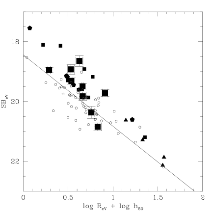
Figure 9: Surface brightness (SB${}_{\textrm{eV}}$) vs. effective radius (R${}_{\textrm{e}}$) for the same sample as in Figure 6 (filled symbols); the large squares are our data, the small squares and the pentagons are the galaxies from CL1358+62 and MS2053-04 (Kelson et al. 1997), and the triangles are the four ellipticals of CL0024 (van Dokkum & Franx 1996). The data of a sample of Coma ellipticals (Lucey et al. 1991) are shown as empty pentagons for comparison, and their best-fit Kormendy relation is overplotted. The mean average offset is $\approx-0.5$ magnitudes. Three galaxies are also shown (B, O, P) for which we have measured photometry and redshift but no central velocity dispersion.

7 Summary

With the instrumental setup and the procedure described Sections 3, 4 and 5, we have measured the Fundamental Plane parameters of intermediate redshift field elliptical galaxies. As an important part of the data-reduction procedure we have carried out accurate K-corrections and spectroscopic aperture corrections. Given the importance of the template spectrum choice for the kinematic fit, we have decided to make use of a wide set of spectra, checking how the results vary with the spectral type, as described in Section 4, obtaining at the same time an estimate of the systematic error produced by the choice of the template spectrum.

While the number of galaxies studied here is too small to draw firm conclusions on the properties of field ellipticals at intermediate redshift, the preliminary evidence suggests that:

1. Our six field ellipticals at redshift $z\sim 0.3$, are in agreement with the local FP relation, with a variation of the zero point ($\Delta\gamma\approx 0.1$), and a scatter of 0.16 in $\log R_{\textrm{e}}$. This means that the stellar populations of our sample of field galaxies are brighter than the local ellipticals, with the same size and mass. This data fit into a scenario in which our galaxies, at a look-back time of $\approx 4$–$5$ Gyrs, are evolving passively. The small sample and the sample selection criteria do not allow any more general conclusion.

2. The FP obtained from our data and the cluster ellipticals at intermediate redshift [van Dokkum & Franx 1996, Kelson et al. 1997] is well defined with a scatter of 0.13 in $\log R_{e}$ with respect to the local relation. The full intermediate redshift sample is large enough to perform the fit the FP coefficients independently. Using the fitting technique used by JFK96, we find $\alpha=0.91$ and $\beta=0.307$, and the scatter is reduced to 0.10. By interpreting the Fundamental Plane as a result of homology, the virial theorem and the existence of a relation $L\propto M^{\eta}$ [van Albada et al. 1995], different slopes at different redshift imply a variation of $\eta$ with time, i.e., a mass-dependent evolution. The good agreement between the field and cluster galaxies suggests that there are no significant differences in the history of the two environments. More data are needed to perform separate fit to the two subsamples.

3. The Kormendy relation between SB${}_{\textrm{e}}$ and $R_{\textrm{e}}$ for all the intermediate redshift data shows an offset of $\approx-0.5$ magnitudes in surface brightness with respect to the Coma ellipticals (L91), in agreement with what is found using the FP. Even though caution is needed, due to possible sample selection biases, the variation of the Kormendy relation suggests that the evolution found via the Fundamental Plane, extends to galaxies at higher redshift. Carefully selected samples of field and cluster intermediate redshift are needed to study the the Kormendy relation in greater detail and to investigate the possible differences between the two environments.

Further discussion on the evolution of elliptical galaxies will be given in a follow-up paper (Paper II; Stiavelli et al. 1999) with the help of information on the line strengths.

8 Acknowledgments

Tommaso Treu’s work at Space Telescope Science Institute (STScI) was financially supported by the STScI Summer and Graduate Student Programs, the Scuola Normale Superiore (Pisa), the Italian Space Agency (ASI), and by STScI DDRF grant 82216. We thank an anonymous referee for several valuable comments which significantly improved the presentation of the kinematic measurement. The use of Gauss-Hermite Fourier Fitting Software developed by R. P. van der Marel and M. Franx is gratefully acknowledged.

References

- [Bender 1990] Bender R., 1990, A&A, 229, 441
- [Bender et al. 1992] Bender R., Burstein D., Faber S. M., 1992, ApJ, 399, 462
- [Bender et al. 1994] Bender R., Saglia R. P., Gerhard, O. E., 1994, MNRAS, 269, 785
- [Bender et al. 1996] Bender R., Ziegler B., Bruzual G., 1996, ApJ, 463, L51
- [Bender et al. 1998] Bender R., Saglia R. P., Ziegler B., Belloni P., Greggio L., Hopp U., Bruzual G., 1998, ApJ, 493, 529
- [Bertin et al. 1994] Bertin G., Bertola F., Danziger J., Dejonghe H., Sadler E., Saglia R. P., 1994, A&A, 292, 381
- [Bruzual & Charlot 1993] Bruzual A. G., Charlot S., 1993, ApJ, 405, 538
- [Burstein & Heiles 1982] Burstein D., Heiles C., 1982, AJ, 87, 1165
- [Capaccioli et al. 1992] Capaccioli M., Caon N., D’Onofrio M., 1992, MNRAS, 259, 323
- [Carollo & Danziger 1994a] Carollo C. M., Danziger I. J., 1994a, MNRAS, 270, 523
- [Carollo & Danziger 1994b] Carollo C. M., Danziger I. J., 1994b, MNRAS, 270, 743
- [Carollo et al. 1997] Carollo C. M., Franx M., Illingworth G. D., Forbes D. A., 1997, ApJ, 481, 710
- [de Carvalho & Djorgovski 1992] de Carvalho R. R., Djorgovski S., 1992, ApJ, 389, L49
- [Dalle Ore et al. 1991] Dalle Ore C., Faber S.M., Jesus J., Stoughton R., 1991, ApJ, 366, 38
- [Davies et al. 1987] Davies R. L., Burstein D., Dressler A., Faber S. M., Lynden-Bell D., Terlevich R. J., Wegner G., 1987, ApJS, 64, 581
- [de Vaucouleurs 1948] de Vaucouleurs G., 1948, Ann. Astrophys., 11, 247
- [Djorgovski & Davis 1987] Djorgovski S., Davis M., 1987, ApJ, 313, 59
- [Dressler 1979] Dressler A., 1979, ApJ, 231, 659
- [Dressler 1984] Dressler A., 1984, ApJ, 286, 97
- [Dressler et al. 1987] Dressler A., Lynden-Bell D., Burstein D., Davies R. L., Faber S. M., Terlevich R. J., Wegner G., 1987, ApJ, 313, 42
- [Faber et al. 1987 1987] Faber S. M., Dressler A., Davies R.L., Burstein D., Lynden-Bell D., 1987, Faber S.M. ed., in “Nearly Normal Galaxies”, Springer, New York, p.175
- [Franx, Illingworth & Heckman 1989] Franx M., Illingworth G. D., Heckman T., 1989, ApJ, 344, 613
- [Griffiths et al. 1994] Griffiths E. et al. 1994, ApJ, 435, L19
- [Holtzman et al. 1995] Holtzman J. A., Burrows C. J., Casertano S., Hester J. J., Trauger J. T., Watson A. M., Worthey G. 1995, PASP, 107
- [Jacoby et al. 1984] Jacoby G. H., Hunter D. A., Christian C. A., 1984, ApJS, 56, 257
- [Jørgensen et al. 1995] Jørgensen I., Franx M., Kjærgaard P., 1995, MNRAS, 276, 1341
- [Jørgensen et al. 1996] Jørgensen I., Franx M., Kjærgaard P., 1996, MNRAS, 280, 167
- [Kelson et al. 1997] Kelson D. D., van Dokkum P. G., Franx M., Illingworth G. D., Fabricant D., 1997, ApJ, 478, L13
- [Kormendy 1977] Kormendy J., 1977, ApJ, 218, 333
- [Kormendy 1982] Kormendy J., 1982, in “Morphology and dynamics of galaxies”, Saas-Fee lessons p. 115
- [Kormendy & Illingworth 1982] Kormendy J., Illingworth G., ApJ, 1982, 256, 460
- [Krist 1994] Krist J., 1994, The Tiny Tim User’s Manual, version 4.0. STScI, Baltimore
- [Lilly et al. 1995] Lilly S., Le Fevre O., Crampton D., Hammer F., Tresse L., 1995, ApJ, 455, 50
- [Lucey et al. 1991] Lucey J. R., Guzmán R., Carter D., Terlevich R.J., 1991, MNRAS, 253, 584
- [Møller et al. 1995] Møller P., Stiavelli M., Zeilinger W. W., 1995, MNRAS, 276, 979
- [Møller & Kjærgaard 1992] Møller P., Kjærgaard P., 1992, A&A, 258, 234
- [Pahre et al. 1995] Pahre M. A., Djorgovski S.G., De Carvalho R.R., 1995, AAS, 187, #110.08
- [Postman et al. 1996] Postman M. et al., 1996, AJ, 111, 615
- [Press et al. 1992] Press W. H., Teukolsky S. A., Vetterling W. T., Flannery B. P., 1992, Numerical Recipes in Fortran; The Art of Scientific Computing, Cambridge University Press, Cambridge
- [Rix & White 1992] Rix H.-W., White S. D. M., 1992, MNRAS, 254, 389
- [Romaniello 1997] Romaniello M., 1997, private communication
- [Sargent et al. 1977] Sargent W. L. W., Schechter P. L., Boksenberg A., Shortridge K., 1977, ApJ, 212, 326
- [Schade et al. 1997] Schade D., Barrientos L. F., López-Cruz O., 1997, ApJ, 477, L17
- [Stiavelli et al. 1993] Stiavelli M., Møller P., Zeilinger W. W., 1993, A&A, 277, 421
- [Stiavelli et al. 1999] Stiavelli M. et al., 1999, in preparation
- [Treu 1997] Treu T., 1997, Tesi di Laurea, Università di Pisa
- [van Albada et al. 1995] van Albada T. S., Bertin G., Stiavelli M., 1995, MNRAS, 276, 1255
- [van der Marel & Franx 1993] van der Marel R. P., Franx M., 1993, ApJ, 407, 525
- [van Dokkum & Franx 1996] van Dokkum P., Franx M., 1996, MNRAS, 281, 985
- [van Dokkum et al. 1998] van Dokkum P., Franx M., Kelson D., Illingworth, G. D., 1998, ApJ, 504, L17
- [Williams et al. 1996] Williams R. E. et al. , 1996, AJ, 112, 1355
- [Worthey 1994] Worthey G., 1994, ApJS, 95, 107
- [Ziegler & Bender 1997] Ziegler B. L., Bender R., 1997, MNRAS, 291, 527