The May 1989 outburst of the Soft X-ray Transient GS 2023+338 (V404 Cyg)

Abstract

We re-analyze archival Ginga data of the soft X-ray transient source GS 2023+338 covering the beginning of its May 1989 outburst. The source showed a number of rather unusual features: very high and apparently saturated luminosity, dramatic flux and spectral variability (often on $\sim 1\,$sec time scale), generally very hard spectrum, with no obvious soft thermal component characteristic for soft/high state.

We describe the spectrum obtained at the maximum of flux and we demonstrate that it is very different from spectra of other soft X-ray transients at similar luminosity. We confirm previous suggestions that the dramatic variability was due to heavy and strongly variable photo–electric absorption. We also demonstrate that for a short time the source’s spectrum did look like a typical soft/high state spectrum but that this coincided with very heavy absorption.

1 Introduction

Low mass X–ray binaries, where a stellar mass black hole or neutron star accretes matter from its Roche Lobe filling companion, are generally transient systems. The mass accretion rate is low enough for the accretion disc to be unstable, leading to long quiescence periods followed by dramatic outbursts (e.g. King et al. 1997a; King, Kolb & Szuszkiewicz 1997b). For the black hole systems, the outburst often shows a rapid rise from a very faint quiescent state, reaching luminosities close to the Eddington limit in a course of a few days. The outburst then declines roughly exponentially, with a characteristic time scale of 30–40 days in both the X–ray and optical flux (e.g. Chen, Schrader & Livio 1997). During the decline the X–ray spectra and variability go through a sequence of well defined states. For luminosities close to the Eddington limit, $L_{\rm Edd}$, the spectrum has both a strong soft component from the accretion disc and a strong power law tail (the very high state). At lower luminosities the hard tail decreases and steepens, so the spectrum is dominated by the soft component (the high state). There is then a dramatic transition, where the soft component decreases substantially in temperature and luminosity, and the spectrum is instead dominated by a hard power law tail (the low state) (see e.g. Tanaka & Lewin 1995; van der Klis 1995; Tanaka & Shibazaki 1996).

GS 2023+338 broke with this pattern in several ways. Firstly, it never clearly showed the very high or high state spectrum even though its luminosity was close to the Eddington limit. Secondly, it showed dramatic flux and spectral variability, part of which can be attributed to a heavy and strongly variable photo–electric absorption (Tanaka & Lewin 1995; Oosterbroek et al. 1997). Thirdly, its optical spectrum was unlike that from any other transient system, with strong, broad lines from H, HeI and HeII: normally these lines are rather weak (Casares et al. 1991).

In this paper we analyze in detail archival Ginga data of GS 2023+338 covering the beginning of its outburst, 23–30 May 1989, attempting to deconvolve the primary spectrum from effects of subsequent reprocessing (absorption, Compton reflection, line fluorescence). The spectrum at the peak luminosity is very different to that seen in more canonical transient systems such as Nova Muscae 1991. We postulate that this spectrum represents super Eddington accretion rates (Inoue 1993), and speculate that this and many of the other peculiar properties of GS 2023+338 are due to the wide separation of the binary, as suggested for GRO J1655–40 (Hynes et al. 1998). The accumulating accretion disc is then very large, so that when the disc instability is triggered there is much more mass in the quiescent disc than in a more typical transient. The accretion can then be super Eddington, giving rise to some form of strong mass outflow which manifests itself as heavy photo–electric absorption, and produces the intense optical line emission. This absorption shrouds the source as the accretion rate declines below Eddington, masking its transition to the standard very high spectrum expected at these luminosities. As the outflow expands with time, the absorption becomes less extreme. Eventually, there are times when the intrinsic source spectrum is not obscured, but by this point the mass accretion rate has declined so that the source is in the low/hard state.

2 Data reduction and background subtraction

Data were extracted from the UK Ginga data archive at Leicester University and reduced in the usual manner. Background subtraction poses a problem for a source as bright and hard as GS 2023+338 since the background monitors (most importantly the Surplus above Upper Discriminator, or SUD) are contaminated by counts from the source. We have used the same method as described in Życki, Done & Smith (1999; hereafter Paper I) to recover the uncontaminated SUD values and then we used the ’universal’ background subtraction method (Hayashida et al. 1989) to estimate and subtract the background. We assume 0.5 per cent systematic errors in the data unless stated otherwise.

Figure 1: Ginga light–curve (count rate in 1–30 keV; 2 sec time bins) on 30th May, when the source’s flux reached its maximum and apparently saturated as well as showed dramatic variability. The count rate was corrected for background, dead-time and aspect. Beginning of good data, $t_{0}$, is 4:31:13. Data for the unabsorbed spectrum (Section 4; Figure 3; Table 1), and for the absorbed one shown in Figure 7 were extracted from time interval $i-1$. Spectra from time intervals $i-4$ and $i-5$ are analyzed in Section 6. They are consistent with soft/high state spectra of SXT, when corrected for absorption.

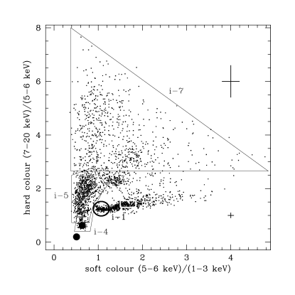
Figure 2: Colour–colour plot for data obtained on 30th May. Time bin is 1 second. The circle marks the region where data for the unabsorbed spectrum were extracted from (Section 4), while the rectangle marks similar region for the absorbed spectrum shown in Figure 7. Contours labeled $i-4$ and $i-5$ mark approximate regions where the soft state data were extracted from (cf. Figure 1; Section 6). Very rapid and chaotic variability was observed during time interval $i-7$, most likely due to photo-electric absorption (Section 5). For comparison, the two big dots show position of Nova Muscae 1991 on January 11 and January 16 (see Section 4.4, Figure 5). The crosses show typical error bars on the colours: the bigger one is for $i-7$, the smaller one for earlier observations.

3 Models

We use a variety of models for spectral description. For the soft component we generally use the multi-temperature blackbody model (Mitsuda et al. 1984). For simple estimates we use the simple version implemented as diskbb in XSPEC. This however does not include the colour temperature correction (e.g. Shimura & Takahara 1995), or the torque-free boundary condition term in the expression for temperature, $1-\sqrt{6R_{\rm g}/r}$ (assuming Newtonian dynamics; Shakura & Sunyaev 1973), where $R_{\rm g}\equiv GM/c^{2}$. We implemented these corrections in a model called diskspec (see also Gierliński et al. 1998). The main parameter can be chosen to be either the temperature at the inner disc radius or the ratio of mass accretion rate and the mass of the central object.

Table 1: Model fitting of the May 30. unabsorbed spectrum.

parameter	units	0	A	B	C
$N_{\rm H}$	$10^{22}\,{\rm cm^{-2}}$	3.7	$0.50^{+0.24}$	$0.50^{+0.13}$	$0.50^{+0.22}$
$kT_{\rm soft}$	keV	0.23	$0.270\pm 0.015$	$0.322\pm 0.015$	$0.281\pm 0.013$
$D_{\rm in}$	$R_{\rm g}$	370	$71^{+15}_{-12}$	$41\pm 8$	$62^{+13}_{-10}$
$\Gamma$		1.57	$1.03\pm 0.04$	$1.690^{+0.023}_{-0.011}\,{}^{a\,b}$	$1.700^{+0.013}_{-0.011}\,{}^{a\,b}$
$E_{c}$	keV	60	$19.6^{+1.2}_{-1.0}$	–	–
$kT_{\rm e}$	keV	–	–	$9.2^{+0.4}_{-0.2}\,{}^{b}$	$9.6^{+0.7}_{-0.5}\,{}^{b}$
$\tau_{\rm es}$		–	–	–	$6.49\pm 0.07\,^{b}$
$T_{0}$	keV	–	–	$0.83\pm 0.03$	$1.44\pm 0.09$
$\Omega_{\rm r}$		–	–	$0.13^{+0.05}_{-0.03}$	$0.17^{+0.16}_{-0.05}$
$\xi$	erg/cm s	–	–	$(2.5^{+7.5}_{-2.0})\times 10^{3}$	$(6^{+18}_{-4})\times 10^{3}$
$R_{\rm in}$	$R_{\rm g}$	–	–	$6^{+1.1}$	$6^{+2}$
$E_{\rm edge}$	keV	–	$7.70\pm 0.13$	–	–
$\tau_{\rm edge}$		–	$1.19\pm 0.13$	–	–
EW	eV	–	$80^{+13}_{-20}$	$67\pm 16$	$70\pm 17$
$\chi^{2}/$dof		555/32	23.5/29	37.3/27	25.7/27

Model 0: absorption*(disc blackbody + cutoff power law)

Model A: absorption*smeared edge*( disc blackbody + cutoff power law + gaussian)

Model B: absorption*(disc blackbody + comptonized blackbody (thComp) + relrepr + gaussian)

Model C: absorption*(disc blackbody + comptonized disc blackbody (thComp) + relrepr +gaussian)

$N_{\rm H}$ – hydrogen column density. Its hard lower limit (interstellar value) is assumed 0.5.
$D_{\rm in}$ – inner disc radius computed from the amplitude of the diskbb model
$kT_{\rm e}$, $\tau_{\rm es}$ – electron temperature and optical depth of the comptonizing cloud
$T_{0}$ – temperature of the seed photon input spectrum for comptonization
$E_{c}$ – e-folding energy in the cutoff power law model
$\Omega_{\rm r},\ \xi$ – amplitude and ionization parameter of the reprocessed component
$R_{\rm in}$ – inner disc radius determining the level of relativistic smearing
EW – equivalent width of the additional gaussian line
${}^{a}\,$ Asymptotic value of $\Gamma$ in the ST80 solution.
${}^{b}\,$ $\Gamma$, $kT_{\rm e}$ and $\tau_{\rm es}$ are of course not independent.
Parameters’ uncertainties are 90 per cent confidence limits for one interesting parameter i.e. $\Delta\chi^{2}=2.71$.

We use an analytic thermal comptonization model to describe the hard component: thComp, based on solution of the Kompaneets equation (Lightman & Zdziarski 1987). For accurate modelling of inverse Compton spectra we also use a Monte Carlo simulation code. It is based on standard methods of simulations of the inverse Compton process as described in detail by Pozdnyakov, Sobol & Sunyaev (1983) and Górecki & Wilczewski (1984) (see Appendix A).

The X–ray reprocessed component is modelled using the angle-dependent Green’s functions of Magdziarz & Zdziarski (1995) convolved with a given continuum model to produce the reflected continuum, with photo–electric opacities calculated by a simple photo-ionization code described in Done et al. (1992). For the iron fluorescent/recombination K$\alpha$ line we used the Monte Carlo code of Życki & Czerny (1994). We constructed Green’s functions for the line emission (i.e. emission for a monochromatic irradiation flux), as functions of ionization and iron abundance, which can be folded with a given continuum model, to compute total line profile, which is then added to the reflected continuum. Parameters of the model are: the amplitude of the total reprocessed component, defined as the solid angle of the reprocessor as seen from the X–ray source, $\Omega$, normalized to $2\pi$, $\Omega_{\rm r}\equiv\Omega/2\pi$ and the ionization parameter, $\xi\equiv 4\pi F_{\rm X}/n$, where $F_{\rm X}$ is the illuminating flux in the 5 eV – 20 keV band and $n$ is the electron number density. We assume cosmic abundances of Morrison & McCammon (1983) with the possibility of a variable iron abundance in the reprocessor. For more model details see Paper I.

The total reprocessed spectrum can then be convolved with the XSPEC diskline model (Fabian et al. 1989; modified to include light bending in Schwarzschild metric) to simulate the relativistic smearing. The main parameter here is the inner radius of the disc, $R_{\rm in}$, assuming a given form of the irradiation emissivity, for which we adopt $F_{\rm irr}(r)\propto r^{-3}$ (see Paper I). The outer disc radius is fixed at $10^{4}\,R_{\rm g}$. This is smaller than the expected outer radius of the disc in GS 2023+338 ($\sim 10^{5}\,R_{\rm g}$; see Section 7.2), but with our assumed $F_{\rm irr}(r)$ the fractional contribution from the ring $10^{4}$–$10^{5}\,R_{\rm g}$ would be negligible, $\approx 5\times 10^{-4}$. The total model will be referred to as relrepr.

Strong photo–electric absorption is modelled by either the simple formula $F\propto\exp(-\tau_{\rm eff})$ where $\tau_{\rm eff}=\sqrt{\tau_{\rm abs}(\tau_{\rm abs}+\tau_{\rm es})}$ (Rybicki & Lightman 1979; called thabs) or by a proper Monte Carlo transmission code for spherical geometry.

We fix the inclination of the source at $i=56^{\circ}$ and assume the mass of the black hole is $12\,{\rm M}_{\odot}$ (Shahbaz et al. 1994). We assume the interstellar $N_{\rm H}=5\times 10^{21}\,{\rm cm^{-2}}$, corresponding to $A_{V}=3$ (Chen et al. 1997; Shahbaz et al. 1994).

The spectral analysis was performed using XSPEC ver. 10 (Arnaud 1996) into which all the non-standard models mentioned above were implemented as local models.

4 The unabsorbed spectrum

On the 30th of May Ginga observed GS 2023+338 in a very bright state (see Fig. 1). The observed source flux reached $6.5\times 10^{-7}$ erg/s/cm² (1 – 40 keV; corresponding to $L_{\rm X}\approx 10^{39}{\rm erg\ s}^{-1}$ at $d=3.5$ kpc) and it apparently saturated at this level. For about 200 sec after the beginning of observation the source spectrum was very stable (Fig. 2) and it did not show any strong photo–electric absorption, so we used the 200 sec average spectrum for detailed analysis.

4.1 Phenomenological description

Generally, the data can be described (Table 1) as a sum of a soft component and a hard cutoff power law component ($\Gamma\approx 1.0$) with e-folding energy of $E_{\rm c}\approx 20\,$keV (i.e. the cutoff is obviously visible in the Ginga band). Superimposed on this are spectral features near 6–10 keV. These features can be phenomenologically modelled by a narrow gaussian at 6.4 keV (EW=77 eV) and the smeared edge (Ebisawa 1991) with $E\approx 7.7\,$keV and $\tau\approx 1.2$ (Model A in Table 1. The presence of the spectral features is highly significant; the best fit model using only two continuum components gives $\chi^{2}=555/32\,$dof (Model 0 in Table 1).

The soft component can be described equally well by both simple blackbody and disc blackbody model. This is due to the fact that only the Wien cutoff is visible in Ginga band. Assuming the model which would give the lowest bolometric correction i.e. a blackbody spectrum and assuming further that at that time there was no photo-electric absorption in excess of the interstellar value, the derived temperature is $kT_{\rm soft}=0.21\,$keV and the normalization of the component corresponds to the emitting area of $\approx 3\times 10^{6}\,{\rm km^{2}}\approx(90\,R_{\rm g})^{2}$. Extrapolated to lower energies, this component then contributes significantly to the total energy budget, with a total bolometric flux of $10^{-6}$ ergs cm^-2 s^-1. Thus the lowest possible luminosity is around the Eddington limit, but it is likely to be rather higher since the soft spectrum must be broader than a single blackbody and the absorption may be rather higher than the (poorly known) interstellar value of $5\times 10^{21}$ cm^-2.

Figure 3: Source spectrum on 30 May, 4:31:13 – 4:34:33 (200 sec), when the flux apparently saturated at very high level (Figure 1, part of time interval $i-1$). The spectrum can be described as optically thick comptonization of a disc blackbody seed spectrum of temperature $kT_{0}\approx 1.4\,$keV, electron temperature $kT_{\rm e}\approx 10\,$keV and $\tau_{\rm es}\approx 6$, with a corresponding reprocessed component (model C in Table 1). An additional soft component is also required: its temperature is rather low: $kT\approx 0.28\,$keV and its amplitude corresponds to inner radius of the emitting disc $\sim 60\,R_{\rm g}$ (for the diskbb model). Counts in the first channel are much above the model contribution suggesting more complicated modelling is necessary. This channel was ignored in spectral fitting.

4.2 Analytical comptonization models

A cutoff power law is not necessarily a good approximation to a comptonized spectrum. We first use the thComp model as an analytic description of the spectrum, including its self–consistently calculated reprocessed spectrum. We also include a separate Fe K$\alpha$ line from fluorescence from distant material. The presence of this was inferred by Oosterbroek et al. (1996) from timing analysis of the May 30th data. Since it is from distant material we fix its energy at 6.4 keV, and assume that it is narrow. We also include a narrow K$\beta$ line at 7.05 keV, tied to 11 per cent of the intensity of the narrow K$\alpha$ line. The best fit thComp model has $\chi^{2}=37.3/27\,$dof, with low electron temperature, $kT_{\rm e}=9.2\pm 0.4\,$keV, rather large optical depth, $\tau_{\rm es}=6.73\pm 0.07$, but requires that the seed photon blackbody temperature is very much higher than that of the observed soft flux, with $T_{0}=0.83\pm 0.04\,$keV. Fixing the seed photons to the temperature of the observed soft excess gives a very much poorer fit as it is unable to reproduce the curvature seen in the hard spectrum at low energies. This best fit model also requires a strongly ionized and smeared reprocessed component, with amplitude $\Omega_{\rm r}\approx 0.13$ (Model B in Table 1)

A significantly better fit can be obtained assuming a broader spectral distribution of the seed photons for comptonization. We have constructed a version of the thComp model in which the input soft photon spectrum is a disc blackbody, rather than a simple blackbody. This model (model C in Table 1), with its corresponding reprocessed component, can now adequately describe the data, with best fit $\chi^{2}=25.7/27\,$dof (i.e. $\Delta\chi^{2}=11.6$ compared to previous case). The comptonizing cloud is rather similar to that derived previously. It is optically thick, $\tau_{\rm es}=6.49\pm 0.07$ and has temperature of $kT_{\rm e}=9.6^{+0.7}_{-0.5}\,$keV. The amplitude of the reprocessed component is much smaller than 1, $\Omega_{\rm r}=0.17^{+0.16}_{-0.05}$, but the reflector properties are nevertheless well constrained. It has to be strongly ionized ($\xi\approx 6000$, so H-like iron ions dominate) and strongly smeared, $R_{\rm in}=6\,R_{\rm g}$. The narrow gaussian at 6.4 keV is still required, its equivalent width is $\sim 70\,$eV. The best fit model spectrum is plotted in Figure 3.

An almost equally good fit ($\chi^{2}=29/27$) can be obtained by replacing the gaussian lines by an unsmeared, neutral reflected spectrum, so it is not possible to distinguish from the spectrum whether the distant material inferred from the timing analysis (Oosterbroek et al. 1996) is optically thick or thin for electron scattering.

Hard lower limit on $N_{\rm H}$ equal to the likely interstellar value of $5\times 10^{21}\,{\rm cm^{-2}}$ was imposed in the above fits. Allowing $N_{\rm H}$ to be a free parameter in model C we actually find that the best fit value is 0, although the fit is now better by only $\Delta\chi^{2}=2.6$ (F-test significance $\approx 90$ per cent). This may indicate possible complexity of the soft component with further evidence for it coming from the observed excess of counts in the first channel (Figure 3). We note however that the excess cannot be solely the result of (unlikely) changes of $N_{\rm H}$ during the integration interval, since the excess remains (although reduced) even if $N_{\rm H}$ is fixed at 0.

4.3 Monte Carlo comptonization models

The analytical solutions for comptonization Green’s functions of Sunyaev & Titarchuk (1980), Lightman & Zdziarski (1987) and Titarchuk (1994) are not accurate when the seed photon energy is close to the plasma temperature, even in the diffusion approximation. Discrepancies also appear close to the plasma temperature (irrespectively of the seed photons energy) as the models are usually not able to correctly reproduce the shape of the high energy cutoff/Wien peak (see e.g. Fig. 2 in Titarchuk 1994). Since in our case the considered energy range is close to both the seed photons energy and plasma temperature, we can expect differences between analytic and simulated spectra.

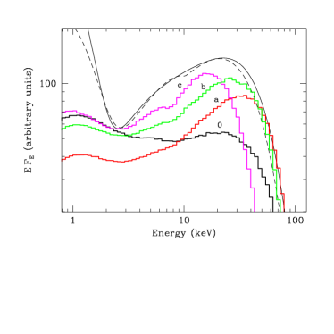
Figure 4: Comptonization spectra in the geometry where the source of seed photons is external to the comptonizing cloud cannot explain the unabsorbed spectrum of GS 2023+338. Solid and dashed curves are best fit models C and 0 (Table 1), respectively. The seed photons spectrum was assumed a disc blackbody of temperature $T_{0}=0.28\,$keV, as observed. Spectrum 0 is for $kT_{\rm e}=11\,$keV and $\tau_{\rm es}=6$, i.e. the same parameters as model C with central source, but with the external illumination the spectrum is much softer. Spectra a, b and c are for $kT_{\rm e}=11,\ 9,\ 5$ keV and $\tau_{\rm es}=8,\ 9,\ 15$, respectively, and are normalized so that they do not exceed the observed spectrum.

However, we demonstrate in Appendix A that for these parameters it is possible to approximate ’exact’ spectra (obtained by Monte Carlo simulations) to better than 1 per cent by the analytical models. The results obtained in previous section are therefore vindicated even though we are not able to do proper fitting of Monte Carlo spectra to the data. The spectral curvature observed in the hard component is not an artifact of the deficiencies of analytic comptonization models. The Monte Carlo spectra also require that the seed photons are at much higher temperatures than those from the observed soft excess.

The analytic and Monte Carlo models compared here both assume that the seed photons are distributed within the comptonizing cloud. However, this is not the case if the hard X–rays form a central source, surrounded by the accretion disc (see e.g. the review by Poutanen 1998 for observational pointers to such a geometry). We computed Monte Carlo spectra assuming a central, spherical plasma cloud of radial optical thickness $\tau_{\rm es}$ and electron temperature $kT_{\rm e}$, surrounded by a geometrically thin disc. The disc is a source of soft photons with a multi-temperature (disc) blackbody spectral distribution parameterized by the temperature at the inner edge, $T_{0}$. These soft photons then form both the observed soft excess spectrum and act as the external illuminating seed photons for the comptonizing cloud. Figure 4 shows examples of inverse Compton spectra obtained in such a geometry. It is not possible to generate a hard and broad enough spectrum in such a geometry, given the constraints on the electron temperature from the observed high energy roll-over and the temperature of the observed soft component. To produce a sufficiently hard spectrum, the optical depth of the cloud has to be large enough for the comptonized spectrum to resemble a Wien peak, which is then rather narrower than the observed spectrum.

Thus it seems inescapable that the comptonized spectrum seen is not produced by scattering the observed soft photons, but rather has as its seed photons a rather higher temperature component which cannot be seen directly (probably because it is embedded in the optically thick comptonizing cloud).

4.4 Comparison with Nova Muscae 1991

The spectral and timing behaviour of GS 2023+338 were quite different from those of Nova Muscae 1991 at the peak of its outburst. Takizawa et al. (1997) examined Ginga data of Nova Muscae 1991 covering first month of its outburst, when the source luminosity was above $\sim 0.5L_{\rm Edd}$. We computed positions of the peak spectrum of GS 2023+338 on their colour–colour and colour–count rate diagrams (their Figure 9bc). The positions are well outside their diagrams, in the directions indicating that the spectrum of GS 2023+338 is much harder than any of the spectra of Nova Muscae below $\sim 10\,$keV, but it is softer than those above this energy. We illustrate this point in Figure 5, where we plot the spectra of both objects: two spectra of Nova Muscae are plotted: one obtained on 11 Jan ($L\approx 0.5L_{\rm Edd}$) and the other on 16 Jan, which has $L\approx L_{\rm Edd}$ (number 1 and 6 in Takizawa et al. 1997; where the outburst of Nova Muscae was first detected on 8 Jan). The latter spectrum has similar luminosity to the peak spectrum of GS 2023+338, yet is very different in shape. For Nova Muscae the soft component is much hotter ($T_{0}=0.87\pm 0.03\,$keV) and dominates the luminosity, while the power law is very soft, $\Gamma=2.76^{+0.08}_{-0.22}$. Even on Jan 11, where the spectrum of Nova Muscae has a strong hard component, its spectrum is much softer than that seen in GS 2023+338 at its peak luminosity. The peak GS 2023+338 spectrum looks similar to the low state spectra seen in both Nova Muscae, GS 2023+338, and other GBH at $L\approx 0.05L_{\rm Edd}$ except for its roll-over at $\sim 20$ keV, and much stronger soft component.

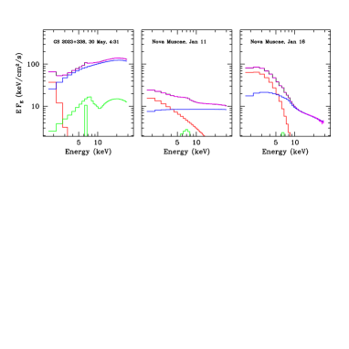
Figure 5: Comparison of energy spectra of GS 2023+338 and Nova Muscae 1991 at peaks of their outbursts. The spectra (Jan 16 of Nova Muscae and the GS 2023+338 one) are very different even though sources’ luminosities (in Eddington units) are very similar and very close to 1. On Jan 11, when $L\approx 0.5\,L_{\rm Edd}$, the soft component cannot be described by a (disc) blackbody – an additional power law tail is required. The strength of the soft component was comparable to that of the hard component. Further increase in $\dot{m}$ results in weakening of the hard component (its slope increases), and strengthening of the soft component which now can be described by the disc blackbody model.

The power spectral density (PSD) of GS 2023+338 during the first 200 s of the $i-1$ interval (excluding the dramatic intensity drop; Figure 6) has intermediate properties between PSDs seen for the two high luminosity spectra of Nova Muscae shown in Figure 5 (cf. Figure 2 in Takizawa et al. 1997, panels 1 and 6). Its shape is close to a power law, which in Nova Muscae seems to correlate with energy spectra being dominated by a thermal component. Its amplitude is however larger, comparable to the amplitude of the (flat-topped) PSD obtained when the energy spectra show strong comptonized power law. This PSD is nothing like that obtained for GBH low state spectra, where the normalized variability amplitude is much larger, at $\sim 0.1$ at 1 Hz. So even though the energy spectrum bears a (rather small) resemblance to the low state spectrum, its variability behaviour clearly shows that it is very different.

Figure 6: Comparison of power spectra of Nova Muscae 1991 and GS 2023+338 at peaks of their outbursts. The same data as for energy spectra (Figure 5) are used. Only data between 1–5 keV are used for the 16. Jan PSD of Nova Muscae.

Both the spectrum and PSD of GS 2023+338 at its peak luminosity look very different from any known spectral state of GBH.

4.5 Discussion

The spectrum and variability of GS 2023+338 at its peak luminosity show that this is very different from any known GBH spectral state. The soft component is at a very low temperature $\sim 0.3$ keV – much lower than expected for a disc which extends down to 3 Schwarzschild radii, accreting at close to (or more probably somewhat above) Eddington limit. The hard component looks like a comptonized spectrum where the electrons have a fairly low temperature since the high energy roll-over can clearly be seen. The parameters of the comptonizing cloud are then fairly well constrained. It has to be optically thick, $\tau=5-6$, with electron temperature $\leq 10$ keV. These electrons scatter an internal source of soft seed photons whose spectral distribution is broader than a blackbody, with maximum temperature $\geq 1$ keV. These are not the same as the much lower temperature ($\sim 0.3$ keV) observed soft excess.

If the seed photons are from the accretion disc then the comptonizing cloud is probably an optically thick corona overlying the accretion disc. This then leads us to a picture where the inner disc is covered by the optically thick comptonizing layers. A rather large extent of the cloud is suggested by simple energetic arguments: since the comptonized spectrum carries $\sim 50$ per cent of the total luminosity, its radius can be expected to be $\sim 25\,R_{\rm g}$, if pure radial stratification of the flow is assumed. We see the normal disc spectrum only from larger radii, which is why the observed soft excess temperature is so much smaller than the $\sim 1$ keV expected from a $12{\rm M}_{\odot}$ black hole accreting at Eddington rates.

The only problem with this picture is that the detected reprocessed spectrum is strongly smeared, to the extent expected if it were reflecting from a disc which extended all the way down to $6R_{\rm g}$. However, the constraints from relativistic smearing can be alleviated if an additional comptonization of the reprocessed component is postulated. Introducing purely phenomenological extension of our model, where the reprocessed component is additionally comptonized in a plasma of temperature $kT_{\rm r}$ and optical depth $\tau_{\rm r}$ (using the Green’s function of Titarchuk 1994 in disc geometry), we obtain a good fit, with $\chi^{2}=19.3/25\,$dof, and the additional plasma parameters $kT_{\rm r}\sim 3.7$keV and $\tau_{\rm r}\sim 2.5$. The reflection amplitude is now $f\sim 0.7$ and the inner disc radius is now unconstrained.

We note that our implementation of the additional comptonization does not correspond to the effect recently emphasized by Ross, Fabian & Young (1998). They point out that the reflected X-rays below $\sim 10$ keV will be comptonized when diffusing through strongly ionized outer layers of the reflecting disc, an effect that is not accounted for in relrepr model (more accurately, this additional comptonization is included in the line profile computations but not in the continuum). While this effect can also be important in our case, as the reflector is indeed strongly ionized, we impose the additional comptonization on the entire reprocessed component, thus changing its overall shape, rather than only below 10 keV.

5 Spectra influenced by strong photo–electric absorption

5.1 The initial variability

After the steady 200 seconds, the flux from GS 2023+338 dropped dramatically. Is this intrinsic variability, or is it caused solely by photo–electric absorption? As a first example we show a 6–seconds averaged spectrum beginning at $t=t_{0}+329\,$s (Figure 1, 2). The spectrum is plotted in Figure 7, together with the unabsorbed spectrum discussed in Section 4. Plainly they are rather similar at the highest energies, but with a factor of $\sim 3-10$ deficit of counts below 15 keV in the later spectrum. This deficit is far too gradual a function of energy to be caused by complete covering by neutral material, so we first use partial covering by heavy absorption, thabs, on a good description of the unabsorbed spectrum (model C in Section 4: disc blackbody and the thComp comptonization model with consistent reprocessing). All the unabsorbed spectral parameters are frozen, except for its overall normalization. This gives a very poor fit to the data, with $\chi^{2}=2028/36$, but including an additional neutral absorber gives a much improved fit with $\chi^{2}=634/35$, where the absorption parameters are: complete covering with $N_{\rm H}\sim 1.6\times 10^{22}$ cm^-2, and partial covering with $N_{\rm H}\sim 3\times 10^{24}$ cm^-2 of 65 per cent of the source. However, the fit underestimates the spectrum in the iron line region and at energies beyond 10 keV. Allowing the additional gaussians to be free gives $\chi^{2}=130/34$, while including the amount of reflection in the fit gives $\chi^{2}=77/33$, for an reflected fraction of $\Omega_{\rm r}\sim 0.7$ and line EW of $\sim 290$ eV (compare with $\Omega_{\rm r}\sim 0.17$ and EW $\sim 70$ eV in the unabsorbed spectrum). The complex neutral absorption then has $N_{\rm H}\sim 10^{22}$ cm^-2 for complete covering and $N_{\rm H}\sim 2\times 10^{24}$ cm^-2 covering 65 per of the source.

Figure 7: Source spectrum (upper panel) on 30 May, 4:36:42 – 4:36:48, ($\Delta t=6$ sec; 329 sec after the beginning of our data), when the flux dropped by a factor of 3 after an initial, very stable level (cf. the light-curve in Figure 1). The spectrum can be described as strongly absorbed spectrum used for the first 200 sec (Figure 3; Section 4). The hydrogen column density is $N_{\rm H}\approx 3.5\times 10^{24}\,{\rm cm^{-2}}$, ionization parameter of the absorber $\xi_{\rm abs}\sim 100$ and the covering fraction $\sim 0.62$. The uppermost dashed curve shows the unabsorbed hard component. Lower panel shows the ratio of data to best fit model. The fit is formally unacceptable, $\chi^{2}=79/33\,$dof, but the residuals do not exceed 5 per cent. They suggest that the absorption cannot be modelled in a single–zone approximation used here.

The apparent changes to the reflection and line emission can be caused by our use of thabs to describe the very heavy absorption. At such high columns, Compton down-scattering can distort the shape of the absorbed spectrum. We replace the analytic approximation by our Monte Carlo transfer code to model the heavy partial absorption. With only the line emission allowed to be free we obtain $\chi^{2}=90/34$, with absorption parameters $N_{\rm H}\sim 1.4\times 10^{22}$ cm^-2, and partial covering with $N_{\rm H}\sim 3\times 10^{24}$ cm^-2 of 62 per cent of the source. For this model, the normalization of the underlying spectrum is less than 5 per cent different to that of the unabsorbed spectrum except that the addition (narrow gaussian) iron line intensity has increased by a factor of $\sim 3$.

The fit can be improved somewhat by allowing the heavy partial absorber to be ionized. This is the best fit spectrum shown in Figure 7. The column density is $N_{\rm H}=3.5\times 10^{24}\,{\rm cm^{-2}}$ i.e. $\tau_{\rm es}\approx 2.8$, $\xi_{\rm abs}\sim 100$ and the covering fraction $\sim 0.6$. However, even this gives $\chi^{2}\sim 79/33$, i.e. the fit is formally unacceptable with residuals at the 5 per cent level. The fit cannot be improved by small changes to the parameters of the primary (comptonized) spectrum or the soft component.

Thus even though the overall spectrum is fairly well explained by the absorption hypothesis, the presence of significant residuals points towards complexity of the absorber. Since the data are an average over a long enough time for the absorber to change, a model involving a range of column densities may be required, rather than a single–zone approximation used here.

5.2 All variability

We use the colour–colour diagram as a guide to the variability. On May 30th the source showed dramatic spectral variability (Figure 2), and this continued during the first month of the decline from outburst (Figure 8). The unobscured spectra are easy to spot on such diagrams, since they fall at the leftmost end of a distinct horizontal track in the colour–colour plots (see also Oosterbroek et al. 1997). The unusual spectrum seen at the unobscured peak outburst luminosity of GS 2023+338 is not the same as the unobscured spectra seen several days later (see Paper I). The unobscured spectra at the end of the absorption track from June 3rd onwards are fairly typical low/hard state spectra (see Paper I), and have inferred luminosities of $\leq 5$ per cent of $L_{\rm Edd}$. Hence there must be some intrinsic spectral and intensity variability as well as the photo–electric absorption.

We will not attempt to construct a full time history of the absorber but will limit our efforts to identifying the spectral components present when the source was in various locations on the colour–colour diagram. Because of the dramatic variability (often on 1 sec time scale), the time intervals over which we summed the spectra are a compromise between requirements of a stable position on the colour–colour diagram and photon statistics. We generally assume that the intrinsic spectrum consists of three components: a soft thermal component which may or may not contribute the seed photons for Compton upscattering to make the hard power law, the comptonized power law and its corresponding reprocessed component. The absorbing material, as well as distorting the intrinsic spectrum, may produce fluorescent line emission, or a reprocessed component of its own.

In the May 30th $i-1$ interval we have shown that the spectral and intensity variability is consistent with complex, heavy absorption. The $i-2$ interval shows similar behaviour to the $i-1$ interval on the colour–colour plot (Figure 2), with strong variability in the soft colour but little change in the hard colour. Thus it seems likely that most of the variability during this interval is also caused by a changing column of the heavy absorption which covers 60–70 per cent of the source, while the intrinsic spectrum remains more or less constant. The variability in the $i-3$ interval is apparently different, starting off in a very low intensity state which is much harder at high energies (approximate position in the diagram $[1.4,2.5]$), which then rises to $[2,3]$, and then rejoins the $i-1$ and $i-2$ absorption track at $\sim[3,1.5]$. However, even here the spectrum is roughly consistent with that of the peak luminosity state (in both shape and intensity), with the heavy absorption changing from a covering fraction of $\geq 90$ per cent at the start to $\sim 70$ per cent as seen in the $i-1$ and $i-2$ intervals at the end.

However, the $i-4$ spectrum is completely different. It cannot be fit by any form of absorption of the peak luminosity spectrum. There is a distinct hard tail, showing that there is indeed some heavy photo–electric absorption, but the low energy spectrum is much softer than that of the peak spectrum (as shown by it having a smaller hardness ratio at low energies). The intrinsic spectrum has changed! We can model this spectrum using a soft component whose temperature is now $\sim 1$ keV. The hard X–ray spectrum is then compatible with these being the seed photons for Compton upscattering, forming a fairly steep power law with $\Gamma\sim 2$, and where the rollover from the electron temperature is not detectable. This is then partially covered by heavy photo–electric absorption. We will discuss the nature of the intrinsic spectrum in more detail in the next section. Here we will merely note its resemblance to the classic high state spectrum (high temperature, steep power law component). The total bolometric unobscured luminosity is then derived to be $\sim 7\times 10^{-8}$ ergs cm^-2, equivalent to $0.07L_{\rm Edd}$.

None of the data taken after this time show a significant high energy rollover, and all have a hard component which can be described by comptonization of the observed soft photons. We use this interval as the starting point (data taken after May 30th 06:30), and plot the colour–colour diagram for all the data up to June 5th (see Figure 8). We have extracted spectra from a number of regions on the colour–colour diagram, and modelled them to try and deconvolve the intrinsic spectrum from the effects of absorption.

During $i-4$ and $i-5$ the source changes mainly in hard colour, making a vertical track (track A) in the colour–colour diagram (Figure 8). This track continues in $i-6$ and $i-7$, but here the spectral variability becomes faster and more chaotic, and includes changes in soft colour as well. Good fits are obtained to spectra i–h–g along track A with a model in which the soft diskbb component has little absorption, while the hard component (Compton scattered power law tail) is more strongly absorbed. In addition, this hard power law illuminates cool, neutral material, giving a reflected spectrum which is even more strongly absorbed, and whose normalisation is strongly enhanced with respect to the observed hard component. Motion from the bottom of track ’A’ to the top corresponds to increasing the enhancement of this reflected component from about a factor 7 at spectrum i to about a factor 100 at spectrum g. The soft spectrum is consistent with remaining fairly constant throughout this track (see Oosterbroek et al. 1997), while the hard component shows the normal broad band variability (see below).

Figure 8: The colour–colour diagram (cf. Figure 2) and examples of spectra influenced by heavy photo–absorption. Solid squares are the source’s positions on May 30th, 6:30–10:00 (i.e. only part of the May 30th data is represented here); small open circles: June 3rd – 5th. The labelled circles mark approximate locations where the spectra were extracted. The spectra are assumed to consist of a soft component modelled as a disc blackbody, absorbed primary power law and its corresponding (but independently absorbed) reprocessed component, together with gaussian lines at 6.4 keV and 7.05 keV (Fe fluorescence), as labelled. Track ’A’ is consistent with both the power law and the reprocessed component being absorbed below $\sim 4$ keV. Movement downwards along the track corresponds to gradual disappearance of the reprocessed component. Horizontal movement corresponds to changes of the normalization of the primary power law. Track ’B’ begins with unabsorbed, low state spectra (position: 1.5, 1.2) and increasing soft colour corresponds to stronger absorption, influencing the primary power law and its reprocessed component.

The total unobscured luminosity at the top of track A is then $\sim 0.5L_{\rm Edd}$ so the inferred luminosity increases by a factor $\sim 10$ from the bottom to top of track A. Yet it seems rather unlikely that this change is actually intrinsic, since the soft component shows very little change in temperature or normalization. It is more likely that the source remains fairly constant at $0.5L_{\rm Edd}$, but that some (variable) amount of the source is completely obscured by optically thick material, and that we see only the intrinsic source spectrum via scattering.

The scattering origin for the observed soft component would be in accord with its small normalization, which is only $\sim 1$ per cent of that expected, if the component indeed is a disc emission from $6\,R_{\rm g}$ onwards. We note here the strong constraints on the scattering scenario for the hard component coming from its observed broad band variability. The high amplitude of the PSD of the hard component ($E>5\,$keV) during the $i-5$ interval (Figure 9) means that the scatterer could not have been located farther than $\sim 0.1$ lsec $\sim 10^{3}\,R_{\rm g}$ (see also next Section).

One geometrical scenario in which to understand these results is that there is a thick disc which blocks our direct view of the source, so that we see only the scattered fraction of the intrinsic radiation. The obscuring wall is axi–symmetric, so there is a strong reflected component of the intrinsic (rather than scattered) emission from the opposite wall. As the disc subsides then we see progressively more of the reflector, so the strength of the hard component increases, giving the variability seen as track A. Eventually the optically thick material goes below our line of sight, allowing the intrinsic hard spectrum to be seen. Differing amounts of fairly heavy absorption on this intrinsic hard spectrum then cause the variability in soft and hard colour defined by spectra g–f–e, but the intrinsic spectrum is consistent with remaining approximately the same in both shape and intensity.

Thus despite the dramatic spectral and intensity variability, the data on May 30th are compatible with very little intrinsic variability. At the start of the observation the source was accreting at (super) Eddington luminosities, with a spectrum unlike any of the known (sub Eddington) spectral states. It then declined by only a factor of $\sim 2$, and made a state transition to the high (or very high) state, and remained at this level for the rest of the observation. All the rest of the variability seen is connected to the absorption.

After the May 30th observation the next data were not taken until 48 hours later, mid-morning of June 1st. These were taken with satellite pointing position which was offset by $\sim 0.8^{\circ}$ from the source, so cannot be used for detailed spectral analysis. However, on the colour–colour plot they span the region around spectrum d. The next good data are taken 12 hours later, on the early morning of June 2nd, where the source spectrum again looks very similar to that of spectrum d. At first sight this looks like a continuation of the g–f–e track, but fitting of the data shows distinct differences. Firstly the overall intensity is rather lower, with the hard component being a factor 10 weaker than in spectrum e. The soft emission is also at much lower temperatures. These, together with the good data taken on June 3-5th form a distinct track in Figure 8 along spectra d–c–b–a (track B) which is not simply connected to track A. Again there must have been some intrinsic spectral change, since the unabsorbed spectra at the end of this track show a classic low state spectral form (Paper I).

Track B can be reproduced by cold partial covering of the Jun 3rd unabsorbed low state spectrum, fixing all the parameters to be the same as in the unabsorbed data (see Paper I). In this model the overall normalization of the June 3rd spectrum (which gives a total bolometric flux of $\sim 4\times 10^{-8}$ ergs cm^-2 s^-1 or $0.04L_{\rm Edd}$) changes by less than 25 per cent while the partial covering absorption parameters change from $3\rightarrow 7\rightarrow 12\times 10^{22}$ cm^-2 covering $\sim 92$ per cent of the source going from spectra a$\rightarrow$b$\rightarrow$c. This confirms the suggestion by Oosterbroek et al. (1997) that the track corresponds roughly to increasing $N_{\rm H}$. We have however used here a much more realistic intrinsic spectrum – the unabsorbed spectrum of the June 3rd data set (Paper I).

The turning point of track ’B’ corresponds to the absorption column of $\approx 1.5\times 10^{23}\,{\rm cm^{-2}}$. Further increasing $N_{\rm H}$ leads to a decrease of the soft colour since it decreases the counts in the 3–5 keV band, whilst the counts in the 1–3 keV band – determined by the soft component – are constant. Thus spectrum d can be fit into the above pattern, with a column of $\sim 31\times 10^{22}$ covering 92 per cent of the source.

6 Has the source ever made a transition to a soft state?

As we point out in Section 5 some of the spectra during May 30th observation show a thermal component of temperature $\sim 0.8\,$keV (for diskbb model) and power law tails with $\Gamma\sim 2$, typical for high/soft states of GBH. To further characterize the source in those time periods we examined more closely some of the energy spectra as well as the source variability.

Figure 9: Power spectra of X-ray emission obtained on two occasions: panel (a) shows PSD on 30th May (time interval $i-5$, 07:26 to 07:48; see Figure 1), panel (b) shows PSD on 20th June when the source was in the usual low/hard state (Paper I). Labels in panel a show energy bands in keV. The thin dotted line represents PSD from panel b for direct comparison. On 30th May the $1-3$ keV component did not vary on time-scales shorter than $\sim 100$ sec, but the amplitude of variability increased with energy. In all three spectra an enhanced variability on time-scales longer than $\sim 100$ sec was observed. This can be attributed to variable photo-electric absorption. On 20th June (panel b) the variability was independent of energy.

6.1 Timing and variability

Power spectra of GS 2023+338 were already examined by Oosterbroek et al. (1997). Their Fig. 8 (panel 1A) shows PSD on May 30 exhibiting strongly reduced power above $\sim 1$ sec, similarly to what is usually observed in high state (van der Klis 1995). In Figure 9a we plot PSD for data obtained between 07:26 and 07:48 ($i-5$; see Figure 1), separately for three energy bands: $1-3\,$keV, $3-5$ keV and $5-30\,$keV. The $1-3$ keV band variability is consistent with pure Poisson noise on time-scales $\delta t\la 100$ sec whilst the harder X-rays are highly variable with the amplitude of variability increasing with energy up to $\approx 5$ keV. For comparison Figure 9b shows PSD for data taken on 20th June (cf. Miyamoto et al. 1992), when the source was in the usual low/hard state (Paper I). Here the amplitude of variability does not depend on energy.

This analysis confirms that the energy spectrum consists of two components, a constant, soft component, and a strongly variable hard component, in accord with spectral decomposition shown in Figure 10.

A characteristic feature of the PSD is the increase of power for $\delta t>100$ sec. Since even the soft component varies on that time-scale, the increase is most likely due to slowly variable absorption.

The PSD of the hard component (5 – 20 keV) on May 30th is rather steeper than that on 20 June for $\delta t\la 10$ sec (frequency $f\ga 0.1$ Hz). The loss of power could be due to reflection/scattering in an extended medium whose presence is suggested both by the energy spectra analyzed in the next section and by the previously discussed increase of PSD on long time-scales. Alternatively, it could be an intrinsic feature of the primary emission. If so, however, then the steepening of PSD in putative soft state would be opposite to what is shown by e.g. Cyg X-1 (van der Klis 1995 and Cui et al. 1997).

6.2 Energy spectra

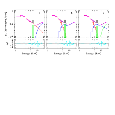
Figure 10: Examples of spectral modelling of the $i-4$ spectrum, when the source was heavily absorbed. Model a is purely phenomenological, comprising two power law spectra absorbed by two (partial) absorbers and an overall absorption. Model b consists of an unabsorbed disc blackbody with $kT\approx 1$ keV, and a power law ($\Gamma\approx 2$) with two absorbers ($N_{\rm H,1}\approx 24$, $f_{1}=1$; $N_{\rm H,2}\approx 300$, $f_{2}=0.86$). Model c has similar disc blackbody, a power law with $\Gamma=2.3$ absorbed by $N_{\rm H}=27$ and $f=1$, and an (enhanced) reprocessed component absorbed by $N_{\rm H}=180$ and $f=1$ (all values of $N_{\rm H}$ are given in units of $10^{22}\,{\rm cm^{-2}}$). Additional narrow gaussian lines at 6.4 and 7.05 keV are included to account for fluorescence in the absorbers. Values of $\chi^{2}$ are, respectively: $21.2/22\,$dof, $20.6/23\,$dof and $17.4/22\,$dof. Only models b and c are compatible with PSD shown in Figure 9a, i.e. the variability increasing with energy up to $\sim 5\,$keV. Parameters of those models are typical for high/soft state of SXT.

We have extracted two spectra of GS 2023+338 from time intervals: $i-4$ at 6:43:45 – 6:47:20 and $i-5$ at 7:26:45 – 7:49:00 (see light-curve in Figure 1, and position on the colour–colour diagram, Figure 2). First, we tested the hypothesis that the spectra can be described assuming (possibly non-uniform) absorption acting on a typical hard state spectrum. To this end we assumed the June 3rd (see Table 2 in Paper I) spectrum and allowed the three components (disc blackbody, power law and reflection) to be absorbed. This model fails in both cases even though we allowed the three absorbers to be different. The best fits have $\chi^{2}=1998/22\,{\rm dof}$ and $\chi^{2}=571/22\,{\rm dof}$. Adding to the model two narrow gaussians at 6.4 and 7.05 keV (to account for iron fluorescence from the absorber) improves the fits significantly but they are still unacceptable: $\chi^{2}=1220/21\,{\rm dof}$ and $\chi^{2}=56.3/21\,{\rm dof}$.

Table 2: Model fitting of the soft state spectra.

data	$kT_{\rm soft}$ (keV)	photon index	$N_{\rm H,1}\,{\rm cm^{-2}}$	$\Omega_{\rm r}$	$\xi$	$N_{\rm H,2}$	EW (eV)	$\chi^{2}/$dof
$i-4$	$1.07^{+0.04}_{-0.11}$	$2.24\pm 0.16$	$(25^{+5}_{-8})\times 10^{22}$	$7.4^{+2.2}_{-1.1}$	$100^{+400}_{-100}$	$(180^{+30}_{-20})\times 10^{22}$	$430^{+70}_{-110}$	17.4/21
$i-5$	$0.98^{+0.03}_{-0.06}$	$1.90^{+0.13}_{-0.11}$	$(24\pm 5)\times 10^{22}$	$6.3^{+1.0}_{-0.8}$	$25^{+40}_{-24.8}$	$(130^{+27}_{-20})\times 10^{22}$	$375^{+75}_{-60}$	15.8/21

Model: abs*( disc blackbody + abs1*(power law) + abs2*(relrepr ) + gaussian + gaussian)

The simplest phenomenological description of the two spectra consists of two power law components with different absorbing columns, $N_{\rm H}$, and covering fractions, $f$, with the two narrow gaussian lines and an overall absorption. One power law is rather soft, $\Gamma\sim 3$ and it is absorbed by a column of $N_{\rm H}\sim(6-8)\times 10^{23}\,{\rm cm^{-2}}$ and $f=0.65-0.9$. The other is harder, $\Gamma\sim 1.2$ while $N_{\rm H}\sim 2\times 10^{24}\,{\rm cm^{-2}}$ and $f=1$.

In an attempt to construct a more realistic model we assumed an unabsorbed disc blackbody as the soft component and an absorbed power law, but such a model fails to describe the data. Better fits are obtained when a second, partial absorption is applied to the power law: $\chi^{2}=20.5/22\,$dof for $i-4$ and $\chi^{2}=27.8/22\,$dof for $i-5$, with the second absorbing column $\sim 3\times 10^{24}\,{\rm cm^{-2}}$. The fit to $i-5$ data can be further improved if the second absorber acts on a different power law component. One realistic candidate for the second power law is the reprocessed component whose presence is also in line with our previous results. Replacing the power law with the (non-smeared) reprocessed component we obtain good fits with $\chi^{2}=17.4/21\,{\rm dof}$ for $i-4$ and $\chi^{2}=15.8/21\,$dof for $i-5$.

The model parameters are well constrained: the temperature of the soft component is fairly high, $T_{0}\sim 1\,$keV, whilst the power law index is $\sim 2$. Both values are indeed as expected in typical high/soft state spectra of GBH. The spectra are plotted in Figure 10 and fit results shown in Table 2.

6.3 Discussion

Based solely on properties of the $i-4$ and $i-5$ spectra it is impossible to determine whether the constancy of the soft component is its intrinsic property or it results from the component (or a fraction of it) being scattered off some extended scatterer towards the observer. The lack of variability is intrinsic if the hard component is scattered as well – as the overall evolution seems to suggest – since the scattering preserved the variability characteristics of the hard component. An intrinsically weak variability then supports the spectral identification of the soft component as the thermal disc emission since this is known to be weakly variable (van der Klis 1995).

The intrinsic luminosity of the soft component is $\approx 9\times 10^{38}\,{\rm erg\,cm^{-2}\,s^{-1}}\approx 0.6\,L_{\rm Edd}$ ($d=3.5\,$kpc), assuming that it indeed is a disc emission from $6\,R_{\rm g}$ onwards. Effective temperature expected at the inner disc edge is then $\approx 1.1\,$keV (Frank, King & Raine 1992), in surprisingly good agreement with the best fit value (fitting the diskspec model with the colour temperature correction 1.5).

The energy spectrum of GS 2023+338 during the $i-4\rightarrow i-7$ time intervals is thus compatible with typical high/soft state spectra of GBH. However, the strong, broad band noise variability of the hard component is not. Examining more closely the Ginga data of Nova Muscae 1991 (see Section 4.4) we find that in the typical high/soft state the hard component ($E>5\,$keV) shows almost no variability, similarly to the soft component (note that in the Ginga data, counts are dominated by channels at 3–5 keV, so the usually plotted – summed over all energies – PSDs are dominated by the soft component). Perhaps a weak intrinsic variability is enhanced by absorption, as suggested by the fact that the PSD amplitude of the soft component was larger later, in $i-7$ than in $i-4$ and $i-5$.

7 Discussion and Conclusions

7.1 Intrinsic X–ray Spectral Evolution

Much of the evolution of the X–ray spectrum is hidden beneath a veil of complex, heavy absorption, and it is not generally possible to uniquely recover the intrinsic spectrum. Most of the dramatic spectral and intensity variability seen on May 30 is connected with the evolution of the complex absorption rather than with the X–ray source itself. The apparent saturation of the X–ray luminosity at $\sim 10^{5}$ counts sec^-1 (see e.g. Figure 1) is not due to the source dramatically flaring and then hitting the Eddington limit, but instead can be explained by the source staying fairly constant while our direct line of sight to it is covered (and uncovered) by very optically thick material.

The absorption variability is such that there are occasional glimpses of the unobscured source. One such time is at the start of the observation on May 30. Here the observed luminosity is at least 0.6 of the Eddington limit (integrating the derived spectrum to get the bolometric luminosity gives the model dependent number of $\geq 1.6\times L_{\rm Edd}$), and the spectral shape is not at all like that seen from other transient systems (at any luminosity!). At these high accretion rates we might expect to see a strong soft component from the inner accretion disc at around $\sim 1$ keV, yet the observed strong soft emission is at temperatures around $0.2$ keV, much lower than expected. The hard X–ray spectrum is not a power law. Instead it has a distinct roll-over, indicating relatively low electron temperatures, $\sim 10$ keV, in the hard X–ray emitting plasma. The curvature of this spectrum is rather difficult to match unless the seed photons for this comptonized spectrum are at temperatures of $\sim 1$ keV. Thus it seems most likely that the missing accretion disc photons are hidden under the optically thick comptonizing cloud which produces the hard X–ray spectrum. Slim disc models (including the advection of trapped radiation) of super-Eddington rates may point towards the formation of such a hot central region (Beloborodov 1998). These extreme luminosities are probably accompanied by a strong wind driven from the disc, which is perhaps the origin of some of the dramatic absorption variability.

The source then makes a transition to the standard very high or high state spectrum, with the expected strong soft component at $\sim 1$ keV. This transition probably takes place between the $i-3$ and $i-4$ time intervals (see Figure 1), perhaps connected to the source luminosity decreasing from $\sim 1.5\times L_{\rm Edd}$ to slightly below $L_{\rm Edd}$. All the May 30th spectra are consistent with an intrinsic bolometric luminosity close to $L_{\rm Edd}$, although this is highly model dependent due to the obscuration of the source.

The source was not observed on May 31, and no good data exist for the observation on June 1st. This is somewhat unfortunate, since on June 2nd the data are consistent with the source having an intrinsic luminosity of $\sim 0.04-0.05\,L_{\rm Edd}$, and show the standard low/hard spectrum. Somewhere in the two missing days the intrinsic source luminosity decreased by a factor of 10–20! The source then decreases by about a factor of 2 from June 2nd to July 6th, consistent with a standard e–folding decay timescale of 30–40 days.

In summary, all of the oddities of GS 2023+338 may perhaps be explained by the source accreting at super-Eddington rates. This would give the unusual spectrum seen at the start of May 30th, and power a strong outflowing wind which caused dramatic absorption variability. As the source declined below Eddington luminosity it showed the standard high state spectrum. It may have further declined steadily (although rapidly) through the high state spectrum to the low/hard state on May 31st–June 1st, or there may have been a more dramatic event, perhaps linked to the observed transient radio emission, in which there was complete disruption of the inner disc. Perhaps this signaled a huge ejection of the accreting matter, so that the accretion rate onto the central object was much reduced, and adding to the complex absorption.

7.2 Disc Evolution

The most promising explanation of SXT outbursts seems to be the classical disc instability model, modified to include the effects of X-ray irradiation (e.g. Cannizzo 1993, van Paradijs 1996, King & Ritter 1998). The quiescent disc builds up from matter accreted from the companion star until the outburst is triggered. The disc switches into the hot, ionized state, and has the familiar Shakura–Sunyaev structure. The outer disc temperature eventually drops below the H ionization temperature, and a cooling wave propagates inwards, switching the disc back into quiescence. Without X–ray irradiation the outburst lightcurves are the classic drawf nova lightcurves, with a linear decline after outburst. However, if X–ray irradiation is strong enough to keep the outer disc ionised then the cooling wave is supressed. Most of the disc mass can then accreted before the cooling wave can form, giving an exponential decay (King & Ritter 1998, King 1998). The prevalence of exponential decays in SXT X–ray lightcurves point to the importance of irradiation in these systems (Shahbaz, Charles & King 1998).

GS 2023+338 shows a fast rise, followed by an exponential X–ray decay. The fast rise suggests that the outburst is triggered towards the outer edge of the disc (Smak 1984, Cannizzo 1998), so that all of the disc takes part in the initial heating wave. The exponential decay means that we might expect that irradiation (probably indirect via scattering in a corona: Dubus et al. 1999) is important so that most of the disc stays in the outburst state, and so is accreted. Integrating the observed X-ray lightcurve gives an estimate of the accreted mass $\Delta M_{\rm X}\sim 6\times 10^{25}\,$g, assuming a radiative efficiency of 10 per cent. This matches very well with estimates of the mass transferred from the companion star during the inter-outburst time interval $\Delta M_{\rm c}\approx 2\times 10^{26}$g, adopting $\Delta t\approx 32\,$years; (Chen et al. 1997) and the mass transfer rate from the companion star $\dot{M}_{\rm c}\approx 10^{17}\,{\rm g\,s^{-1}}$ (King, Kolb & Burdieri 1996).

However, this disc mass is orders of magnitude smaller than the disc mass that would be built up under the assumption that the outburst is triggered by the surface density of the quiescent disc reaching its critical value everywhere. The orbital period of GS 2023+338 is 6.5 days, so the disc can extend out to radii of $R_{\rm out}\simeq 1.36R_{\rm circ}\approx 0.7R_{\rm tidal}\approx 1.2\times 10^{12}$ cm (Shahbaz et al. 1998). This predicts a huge disc mass of $M_{\rm disc}\sim\rho R_{\rm out}^{3}/3\sim 2\times 10^{28}$ g ($\rho\sim 3\times 10^{-8}\,{\rm g\,cm^{-3}}$; King & Ritter 1998). Plainly this shows that the outburst is triggered long before this maximum disc mass is built up. A similar result is found for the other well studied large disc system, GRO J1655-40 (Shahbaz et al. 1998). This is in marked contrast the to short period (small disc) SXT’s, where the disc mass derived from the maximum quiescenct disc calculations is (roughly) equal to the mass inferred from the X–ray luminosity (Shahbaz et al. 1998), and to the integrated mass transfer rate from the companion star (Menou et al. 1999). Perhaps a clue to resolving the problem is that the region where the disc solution is unstable in GS 2023+338 is quite distant from $R_{\rm out}$. Solving the vertical disc structure equations (using the code recently described in Różańska et al. 1999), we find that the solution is unstable where $T_{\rm eff}=(5-7)\times 10^{3}\,$K (see also e.g. Hameury et al. 1998). This gives $R_{\rm unst}=(5-8)\times 10^{10}\,$cm, i.e. the ring is centered at $\approx 0.05\,R_{\rm out}$. In Nova Muscae 1991 ($P_{\rm orb}=10.5\,$h) $R_{\rm unst}$ is rather closer to $R_{\rm out}$: $R_{\rm unst}=(2-3)\times 10^{10}\,{\rm cm}=(0.2-0.3)R_{\rm out}$. Perhaps the disc beyond a few $R_{\rm unst}$ never builds up to full quiescence, but instead stays on the steady state, cool branch. Whatever the reason, it seems that there are serious deficiencies in our understanding of the structure of large discs.

Appendix A Differences between Monte Carlo and analytic solutions of the comptonization problem and their influence of modelling the reprocessed spectra

Figure 11: Comparison of the best analytical (Titarchuk 1994) and Monte Carlo solutions of comptonization Green’s functions. Panel (a): $kT_{0}=0.1\,$keV, $kT_{\rm e}=100\,$keV, $\tau=1$; (b): $kT_{0}=0.3\,$keV, $kT_{\rm e}=100\,$keV, $\tau=0.4$; (c): $kT_{0}=1\,$keV, $kT_{\rm e}=10\,$keV, $\tau=6$. Upper panels show the Green’s functions, lower ones their ratio (normalized to 1 at 2 keV). The comptonizing cloud is assumed to be spherical, and seed photons spatial distribution follows $\propto\sin(\tau)/\tau$. Errors on Monte Carlo spectra are standard deviations of 6 averaged spectra, each using $2\times 10^{6}$ (a), $4\times 10^{6}$ (b) and $10^{6}$ (c) photons.

Figure 12: Results of fitting ’fake’ data created from Monte Carlo comptonization spectra by two analytical comptonization models: thComp and comptt. Parameters of the Monte Carlo spectra are the same as in Figure 11 except for the seed photons spectrum which is a blackbody here. As can be seen, the Monte Carlo spectra can usually be quite well reproduced by adjusting parameters in the analytical models.

Analytical approximation to comptonization problem are usually not accurate at energies close to the seed photons or plasma temperatures (e.g. Skibo et al. 1995). We have therefore investigated whether the differences between “accurate” spectra, computed using a Monte Carlo code, and analytical approximations (which we normally use in data fitting) may influence our conclusions regarding the reprocessed component, in particular the inferred ionization and the level of relativistic smearing.

Our Monte Carlo comptonization code is written following closely the description given by Pozdnyakov, Sobol & Sunyaev (1983) and Górecki & Wilczewski (1984). One modification we have made is to replace the analytical approximations to $F(x)\equiv(2\pi r_{0}^{2})^{-1}\,\int_{0}^{x}\,y\sigma(y)\,dy$ (where $\sigma(x)$ is the scattering cross-section as function of photon energy) and its inverse function (see Eq. A8 and A13–A15 in Górecki & Wilczewski 1984) by values computed numerically and then interpolated.

To demonstrate the (in)accuracy of analytical solutions of the comptonization problem we first show in Figure 11 the Green’s functions for three cases: a $kT_{\rm e}=100\,$keV, $\tau_{\rm es}=1$, $kT_{0}=0.1\,$keV (typical low/hard state spectra of GBH), b $kT_{\rm e}=100\,$keV, $\tau_{\rm es}=0.4$, $kT_{0}=0.3\,$keV (high/soft state of Nova Muscae 1991; Życki, Done & Smith 1998) and c $kT_{\rm e}=10\,$keV, $\tau_{\rm es}=6$, $kT_{0}=1\,$keV (peak spectrum of GS 2023+338; Section 4). In all cases the comptonizing cloud is a uniform sphere, with sources’ distribution given by $\propto\sin(\tau)/\tau$ (Sunyaev & Titarchuk 1980). The analytical model is that of Titarchuk (1994) which we found best agrees with the Monte Carlo spectra for given $kT_{\rm e}$ and $\tau$ in the broad range of parameters we are considering.

The most certain way of testing possible influences would obviously be to fit the data by a Monte Carlo model and compare the results with those obtained with analytical approximations. This being impossible in practice, we adopted following procedure: we created fake ’data’ from comptonization spectra computed using our Monte Carlo code. The Ginga response matrix (for summed top and mid layers; Turner et al. 1989) was used to create the data and their statistical quality is similar to our real data. We then attempted to fit the analytical models to the data in the 2-30 keV range. We assume the same parameters as for the Green’s functions except for the seed photons spectrum for which we now assume a blackbody.

Figure 12 shows results of fitting two analytical models: thComp and comptt to the fake data. In the cases a and b we fixed the plasma temperature in the models to the value used in Monte Carlo simulations since using data only up to 30 keV does not allow $kT_{\rm e}$ to be constrained. The best fit optical depth is then $\approx 1.2$ in case a and 0.5-0.7 in case b. As can be seen, residuals up to 4 per cent can still be present. High temperature, optically thin spectra are most difficult to reproduce as the analytical models usually assume a diffusion approximation for photon escape. Fitting the data corresponding to low/hard state gives much better results, with residuals not exceeding 2 per cent. We note remarkably good fit of the thComp model to Monte Carlo spectrum characteristic to GS 20223+338 at its peak (panel c), with the model parameters within $\sim 10$ per cent of the original values. The reason for the bad fit of the comptt model in this case seems to be that the seed photons spectrum is taken as the Wien spectrum rather than a blackbody used originally.

The residuals observed in the above fits may indeed have some influence on results of modelling the reprocessing. To asses the influence, we attempted to improve the fits by adding a reprocessed component to thComp model. Results of fitting real data by models containing reprocessing could be affected, if indeed such a composite spectrum was able to mimic the complexity of ’real’ comptonization. This does not however seem to be the case. For low/hard state spectra we found that the reprocessed component (with $\xi$ fixed at 0, as for typical real data) cannot improve the fit, i.e. the difference between Monte Carlo and analytical comptonization cannot be ’filled in’ by a reprocessed component. For high/soft state we indeed see that an ionized and smeared reprocessing, with amplitude $\Omega_{\rm r}\approx 0.05$ can reduce some of the residuals. We thus added such a component to our basic model of reprocessing and we repeated fits to high state spectrum of Nova Muscae 1991, obtained on 18th May (Życki et al. 1998). The resulting $\chi^{2}$ contours in the $\Omega_{\rm r}$–$R_{\rm in}$ plane is shifted by $\sim 0.06$ towards smaller values but its overall shape remains unchanged. We thus conclude that the small differences between Monte Carlo and analytical models of comptonization are not able to change conclusions regarding properties of the X–ray reprocessed component in our spectra.

We finally note that the above discussion is relevant only if a single value of electron temperature is assumed. In more realistic models, where accretion flow dynamics as well as radiative transfer are considered, a range of temperatures can be expected. This will inevitably change the details of the spectrum and the above discussion.

References

- [] Arnaud K. A. 1996, in Astronomical Data Analysis Software and Systems V, eds. Jacoby G. and Barnes J., ASP Conf. Series volume 101, p. 17
- [] Beloborodov A. M. 1998, MNRAS, 297, 739
- [] Cannizzo J. K. 1993, in Accretion Disks in Compact Stellar Systems, ed. J. C. Wheeler (Singapore: World Scientific), p. 6
- [] Cannizzo J. K. 1998, ApJ, 494, 366
- [] Casares J., Charles P. A., Jones D. H. P., Rutten R. G., Callanan P. J. 1991, MNRAS, 250, 712
- [] Chen W., Shrader C. R., Livio M. 1997, ApJ, 491, 312
- [] Cui W., Zhang S. N., Focke W., Swank J. H. 1997, ApJ, 484, 383
- [] Done, C., Mulchaey, J. S., Mushotzky, R. F., Arnaud, K. A. 1992, ApJ, 395, 275
- [] Dubus G., Lasota J.-P., Hameury J.-M., Charles P. 1999, MNRAS, 303, 139
- [] Ebisawa K., 1991, PhD thesis, Univ. of Tokyo
- [] Fabian A. C., Rees M. J., Stella L., White, N. E. 1989, MNRAS, 238, 729
- [] Frank J., King A. R., Raine D. 1992, Accretion Power in Astrophysics (Cambridge:Cambridge Univ. Pres)
- [] Gierliński M., Zdziarski A. A., Poutanen J., Coppi P., Ebisawa K., Johnson W. N. 1998, MNRAS, submitted
- [] Górecki A., Wilczewski W. 1984, Acta Astron., 34, 1
- [] Hameury J.-M., Menou K., Dubus G., Lasota J.-P., Huré J.-M. 1998, MNRAS, 298, 1048
- [] Hayashida K., Inoue H., Koyama K., Awaki H., Takano S., 1989, PASJ, 41, 373
- [] Hynes R. I. et al. 1998, MNRAS, 300, 64
- [] Inoue H. 1993, in Accretion Disks in Compact Stellar Systems, ed. J. C. Wheeler
- [] King A. R. 1998, MNRAS, 296, L45
- [] King A. R., Frank J., Kolb U., Ritter H. 1997a, ApJ, 484, 844
- [] King A. R., Kolb U., Burdieri L, 1996, ApJ, 464, L127
- [] King A. R., Kolb U., Szuszkiewicz E., 1997b, ApJ, 488, 89
- [] King A. R., Ritter H. 1998, MNRAS, 293, L42
- [] Lightman A. P., Zdziarski A. A. 1987, ApJ, 319, 643
- [] Magdziarz P., Zdziarski A. A., 1995, MNRAS, 273, 837
- [] Menou K., Narayan R., Lasota J.-P. 1999, ApJ, 513, 811
- [] Mitsuda K. et al., 1984, PASJ, 36, 741
- [] Miyamoto S., Kitamoto S., Iga S., Negoro H., Terada K. 1992, ApJ, 391, L21
- [] Morrison R., McCammon D., 1983, ApJ, 270, 119
- [] Oosterbroek T. et al. 1996, A&A, 309, 781
- [] Oosterbroek T. et al. 1997, A&A, 321, 776
- [] Poutanen J., 1998, in Abramowicz M. A., Björnsson G., Pringle J. E., eds, Theory of Black Hole Accretion Discs, CUP, Cambridge, in press, (astro-ph/9805025)
- [] Pozdnyakov L. A., Sobol I. M., Sunyaev R. A. 1983, Ap. Space Phys. Rev., 2, 189
- [] Ross R. R., Fabian A. C., Young A. J. 1998, MNRAS, in press
- [] Różańska A., Czerny B., Życki P., Pojmański G. 1999, MNRAS, in press
- [] Rybicki G. B., Lightman A. P. 1979, Radiative Processes in Astrophysics. John Wiley & Sons, New York
- [] Shahbaz T., Ringwald F. A., Bunn J. C., Naylor T., Charles P. A., Casares J., 1994, MNRAS, 271, L10
- [] Shahbaz T., Charles P. A., King A. R. 1998, MNRAS, 301, 382
- [] Shakura N. I., Sunyaev R. A. 1973, A&A, 24, 337
- [] Shimura T., Takahara F. 1995, ApJ, 445, 780
- [] Skibo J. G., Dermer C. D., Ramaty R., McKinley J. M. 1995, ApJ, 446, 86
- [] Smak J. I. 1984, Acta Astron., 34, 161
- [] Sunyaev R. A., Titarchuk L. N. 1980, A&A, 86, 121
- [] Titarchuk L. 1994, ApJ, 434, 570
- [] Takizawa M. et al. 1997, ApJ, 489, 272
- [] Tanaka Y., Lewin W. H. G. 1995, in X–Ray Binaries, ed. W. H. G. Lewin, J. van Paradijs & E. van den Heuvel (Cambridge: Cambridge Univ. Press), 126
- [] Tanaka Y., Shibazaki N. 1996, ARA&A, 34, 607
- [] Turner M. et al. 1989, PASJ, 41, 345
- [] van Paradijs J. 1996, ApJ, 464, L139
- [] van der Klis M. 1995, in X–Ray Binaries, ed. W. H. G. Lewin, J. van Paradijs & E. van den Heuvel (Cambridge: Cambridge Univ. Press), 252
- [] Życki P. T., Czerny B., 1994, MNRAS, 266, 653
- [] Życki P. T., Done C., Smith D. A. 1998, ApJ, 496, L25
- [] Życki P. T., Done C., Smith D. A. 1999, MNRAS, 305, 231 (Paper I)