A Study of the $B-V$ Colour Temperature Relation

Abstract

We attempt to construct a $B-V$ colour temperature relation for stars in the least model dependent way employing the best modern data. The fit we obtained with the form $T_{\rm eff}=T_{\rm eff}((B-V)_{0},[{\rm Fe/H}],\log g)$ is well constrained and a number of tests show the consistency of the procedures for the fit. Our relation covers from F0 to K5 stars with metallicity [Fe/H]=$-$1.5 to +0.3 for both dwarfs and giants. The residual of the fit is 66 K, which is consistent with what are expected from the quality of the present data. Metallicity and surface gravity effects are well separated from the colour dependence. Dwarfs and giants match well in a single family of fit, differing only in $\log g$. The fit also detects the Galactic extinction correction for nearby stars with the amount $E(B-V)=0.26\pm 0.03$ mag/kpc. Taking the newly obtained relation as a reference we examine a number of $B-V$ colour temperature relations and atmosphere models available in the literature. We show the presence of a systematic error in the colour temperature relation from synthetic calculations of model atmospheres; the systematic error across K0 to K5 dwarfs is 0.04$-$0.05 mag in $B-V$, which means 0.25-0.3 mag in $M_{V}$ for the K star range. We also argue for the error in the temperature scale used in currently popular stellar population synthesis models; synthetic colours from these models are somewhat too blue for aged elliptical galaxies. We derive the colour index of the sun $(B-V)_{\odot}=0.627\pm 0.018$, and discuss that redder colours (e.g., 0.66-0.67) often quoted in the literature are incompatible with the colour-temperature relation for normal stars.

1 Introduction

The determination of the stellar locus in the HR diagram is a subject of the prime importance in astrophysics, as well as it has wide applications. For instance, the determination of the distance scale relies much on the uniqueness of the stellar locus. Such work has often resorts to the knowledge of theoretical isochrones, since the observations alone do not span sufficiently large parameter space. On the other hand, theoretical isochrones, expressed in the colour-magnitude space, may suffer from errors of three origins. The errors may arise from (i) evolution track calculations which depend on opacity, nuclear reaction rate, equation of states and the treatment of convection, (ii) conversion of temperature to colour index (colour-temperature relation), and (iii) conversion of luminosity to magnitude in a specific passband (bolometric corrections). The recent findings of the difference in the distance to open clusters by Hipparcos parallax as compared to the traditional zero age main sequence (ZAMS) fitting (van Leeuwen & Hansen Luiz 1997; van Leeuwen 1999; Mermilliod et al. 1997; Pinsonneault et al. 1998) have tempted us to study the problem of reliability concerning theoretical isochrones. An analysis of Nordström, Andersen & Andersen (1997) indicates that the discrepancy of the isochrones among different authors can be as much as 0.4$-$0.6 mag, although in most practical applications the isochrones are used so that such a large error does not directly affect the results. Their figures also indicate that a dominant part of the errors may arise from the colour-temperature relation, especially when $B-V$ colour is used, as we have also confirmed from our own analysis. The error arising from the bolometric correction is rather small, and the evolution track on the luminosity temperature plane is reasonably converged among authors, in so far as we are concerned with the region far from the turn-off point where convective overshooting may start making a difference.

Another particularly important application of the stellar track is stellar population synthesis of galaxy colours, which play an important role in cosmology (e.g., Tinsley & Gunn 1976; Bruzual & Charlot 1993; Kodama & Arimoto 1997). If colour of giant stars would contain errors as much as $\Delta(B-V)>0.05$, the interpretation of elliptical galaxies could significantly be disturbed.

In this paper we focus on the problem of the colour-temperature ($T_{\rm eff}$) relation. We attempt to construct the relation, which we think the least model dependent, and study what errors are contained in the existing relations. There are a lot of work for the colour-temperature relation. The early authority is the one given by Johnson (1966), and the work to 1980 is summarised by Böhm-Vitense (1980). We also quote several representative examples, which include Code et al. (1976), Blackwell & Shallis (1977), Bessell (1979), Ridgway et al. (1980), Saxner & Hammarbac̈k (1985), Arribas & Martínez-Roger (1988), Tsuji et al (1995) and Di Benedetto & Rabbia (1987). Most recent work includes Flower (1996), Alonso et al. (1996b), Blackwell & Lynas-Gray (1998; hereafter BL98), and Lejeune, Cuisinier & Buser (1998).

The prime difficulty lies in estimating precise temperature. The most direct method employs the measurement of angular diameter of stars using interferometry or lunar occultations. The number of stars which are given accurate angular diameters are increasing (Davis 1998), especially with the advancement of the Michelson interferometry technique, but not yet sufficiently many to explore large parameter space.

One of the methods which are supposed to be accurate and often used in modern literature is the infrared flux method (IRFM), in which $T_{\rm eff}$ is estimated from the measurement of $R=F_{\rm bol}/F_{\lambda}=\sigma T_{\rm eff}^{4}/\psi(\lambda)$ for infrared $\lambda$, where $\psi(\lambda)$ is calculated from model atmospheres (Blackwell & Shallis 1977). This method has been developed to reduce the model dependence using the fact that $F_{\lambda}$ in the near infrared regions is smoothly proportional to $T_{\rm eff}$ and model dependence is fairly small. Alonso, Arribas & Martínez-Roger (1996a,b) and BL98 have given the latest and most extensive work employing this method.

Mégessier (1994) and Alonso et al. (1996a) have examined the error associated with this method. The authors of both papers claim that the derived temperature differs as much as 100K depending on the model atmosphere employed in the work. For example use of ATLAS9 (Kurucz 1993) gives temperature 100K higher than ATLAS8. Similar difference is also reported between MARCS (Gustafsson et al. 1975 and their updates) and ATLAS9.

An important advancement is brought by Di Benedetto (1998; hereafter B98) who found an empirically very tight relationship between $T_{\rm eff}$ and $V-K$ colour, which is calibrated with the direct angular diameter measurement. He has shown that this relationship depends very little on luminosity class and metal abundance. This makes possible to estimate temperature for F-K dwarfs, for which direct measurements of diameters are still lacking. This method would offer the least model-dependent method to deal with a fairly large sample without a direct angular size measurement for each star.

We have examined the accuracy of the B98 temperature, and are convicted that it is perhaps the best method available to us for the time being. B98, however, has not discussed much with $B-V$ colour, which is very sensitive to line blanketing and also to surface gravity, giving a large scatter around the surface brightness colour relation. This is also true with a recent comparative study of Bessell, Castelli & Plez (1998), who extensively compared model atmosphere calculations with empirically estimated $T_{\rm eff}$ for various colour bands, but except for $B-V$. On the other hand, most of the applications of the stellar locus still rely predominantly on $V$ magnitude and $B-V$ colour.

For this reason we attempt to construct a $B-V$ colour temperature relation adopting the $T_{\rm eff}$ data from B98 together with an extensive photometric database compiled by Hauck & Mermilliod (1998), combined with the metallicity and log $g$ data compiled by de Strobel et al. 1997 (hereafter SSFRF) for F0-K7 stars. We also examine the available $B-V$ colour temperature relations, especially those published recently, against what we have constructed in order to find external errors of these works. Further examination is also made for the colour-temperature relation used by theoretical work of stellar evolution, which is often used as a basis to discuss the cosmic distance scale and age, as well as taken as a fiducial for stellar population synthesis for colour of galaxies. As for the required accuracy for the distance work, if our goal is to obtain a 3% accuracy in the distance estimation, one would need to achieve the accuracy of $B-V$ to be 0.01 mag, which in turn is translated to temperature error of 20$-$45 K. In our paper we attempt to document the error budget arising from many components of the input data. This would clarify the limiting factor to the accuracy of the $B-V$ colour temperature relation and tell us what improvement should be done to go further. We shall see that the accuracy that we can achieve is worse than this goal by about a factor of 2$-$3 for each star. When many stars in clusters are averaged, however, the accuracy is of the order of 0.015 mag in $B-V$.

One of our additional aims is to extract the dependence of the $B-V$ colour temperature relation on metallicity, without resorting to theoretical grids, and in particular to examine the accuracy of synthetic results from model atmospheres. As a byproduct this makes possible to estimate colour of the sun from solar analogues (e.g., Taylor 1998; de Strobel 1996 for reviews).

In section 2, we derive the $B-V$ colour temperature relation, after examining the quality and reliability of input data. We also present a table of the estimated error budget. In section 3, an extensive comparison is made with the existing $B-V$ colour temperature relations based on either empirical or theoretical ground. We discuss in section 4 $B-V$ colour of the sun. Metallicity dependence is discussed in section 5. Our conclusion is given in section 6.

2 Construction of the $B-V$ colour temperature relation

2.1 Data

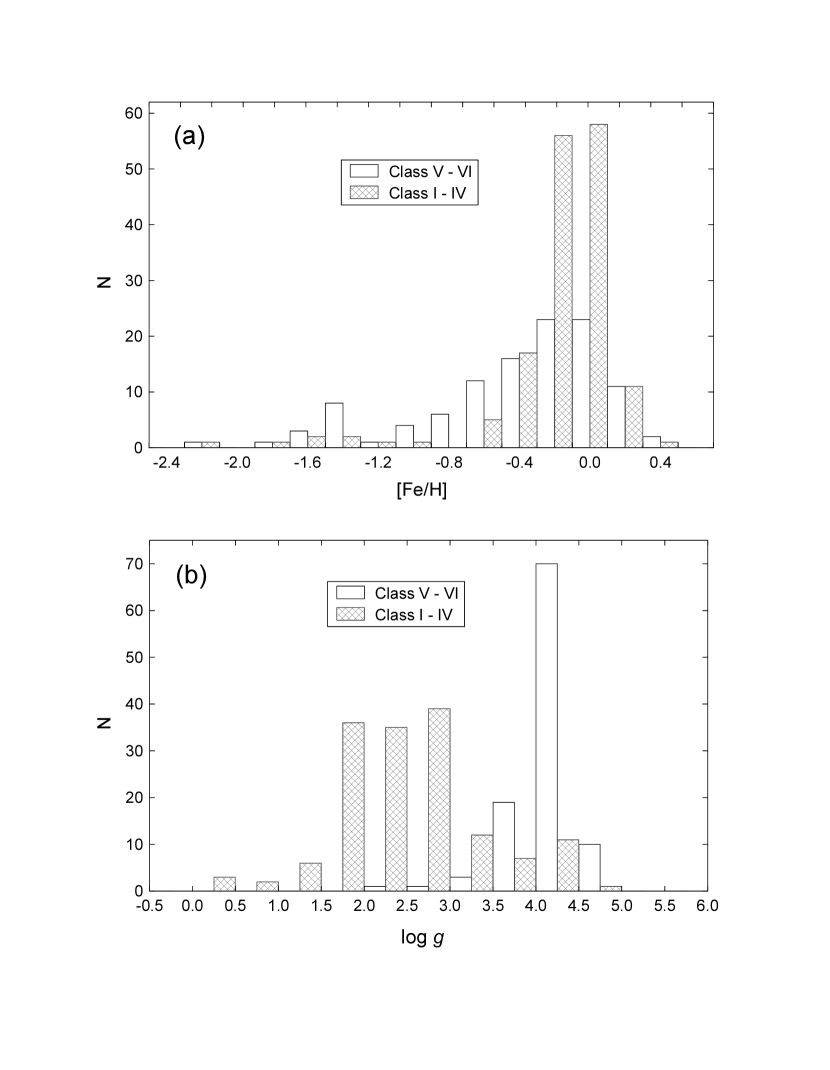
Figure 1: Distribution of (a) [Fe/H] and (b) $\log g$ for the 270 stars used in our analysis.

To derive a relation between $T_{\rm eff}$ and $B-V$ colour, we start with 537 ISO standard stars for which B98 has given accurate estimates of $T_{\rm eff}$. Of those 537 starts, 270 stars are given estimates of [Fe/H] and $\log g$ by SSFRF. Among them about 40% (110 stars) are dwarfs or subdwarfs and 60% (160 stars) are giant stars. For a majority of entries SSFRF gives more than one data for [Fe/H] and $\log g$ for a given star; in such cases we take median values of [Fe/H] and $\log g$. The distributions of the median values of [Fe/H] and $\log g$ are shown in Figs. 1 (a) and (b). The data are distributed widely from [Fe/H] =$-$2.0 to +0.5; only 10% of stars have [Fe/H] $<-1.0$, but we still have a reasonable number of stars to constrain our analysis in this region. The ten percentile for the metal rich side is [Fe/H] $=0.12$. All stars of our sample are given $B-V$ colours (Hauck & Mermilliod 1998) and parallaxes with Hipparcos (ESA 1997).

We give in Table 1 the derivative of $T_{\rm eff}$ against $B-V$ to obtain an idea about the propagation of errors from $T_{\rm eff}$ to $B-V$. The table gives $\Delta T_{\rm eff}$ that causes a change of $\Delta(B-V)$=0.01. For instance, $\Delta T_{\rm eff}=45$K is an allowance for F0 stars (7000K); it is 30 K for G2 stars, and 16K for K5 stars at 4000 K.

2.2 Examination of B98’s temperature estimates

None of the temperature estimates are completely free from the atmosphere model. Spectroscopic determinations of temperature directly rely on the details of the atmosphere model, and IRFM uses the prediction of the atmosphere model in the near infrared region. Even the direct measurement of angular diameters should be supplemented with the atmosphere model, albeit with a minimal extent, in order to estimate the bolometric flux in the invisible regions. The method proposed by B98 basically belongs to this last category. He found a tight correlation between surface brightness and $V-K$ colour (dispersion being 0.03 mag) to estimate angular size $\phi$, and used another tight relationship between the bolometric flux $F_{\rm bol}$ and $V-K$ colour found by BL98 to estimate effective temperature of stars for which the direct measurements are not available for $\phi$ and $F_{\rm bol}$.

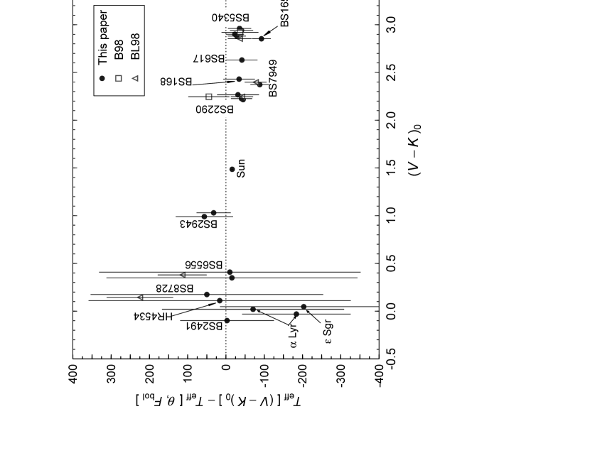
Figure 2: Examination of temperature given by B98. The difference $\Delta T_{\rm eff}=T_{\rm eff}[(V-K)_{0}]-T_{\rm eff}({\rm reference})$ (B98) is plotted as a function of $(V-K)_{0}$. The data points used by B98 for his own examination and temperature given in BL98 are also plotted. The data actually used in our analysis is confined to $(V-K)_{0}\geq 1.0$.

Since it is of crucial importance to examine the accuracy of effective temperature estimated with this method, we plot in Fig. 2 the difference of temperature given by B98 from $V-K$ colours and that obtained directly using

$$T_{\rm eff}^{4}=\frac{4}{\sigma}\phi^{-2}F_{\rm bol},$$ (1)

which is equivalent to the defining equation for effective temperature. Here $\sigma$ is the Stefan-Boltzmann constant. The table given by B98 (Table 3) contains all angular size measurements which could be used for our test (21 stars and the sun). We take the bolometric flux from direct evaluations of several sources, as presented in Table 2. The bolometric flux is an integration of flux from $U$ to $K$ bands with shorter and longer wavelength ranges evaluated with the aid of atmosphere models. The direct integration accounts for 93% of flux at $T$=4500K, and 83% at 7000K (Alonso et al 1995). Therefore, the dependence on model atmosphere is expected to be quite small. It is expected that the error is no more than 2% for the bolometric flux, which means a 0.5% error in $T_{\rm eff}$. We also note that there is an error of this order (1.5%) in the absolute calibration of flux of $\alpha$ Lyr at 5556Å (Hayes 1985). We explicitly document the calibrations employed by the respective authors in Table 2 (ref/norm), but do not dare to adjust to the same scale, since the difference is smaller than errors of other origins. Among 22 stars of B98 direct bolometric flux estimates are available for 16 stars. We take each estimate by different authors as an independent data, so that 32 data points are contained in Fig. 2. The errors attached to our $T_{\rm eff}$ are obtained by a quadrature of the errors for $F_{\rm bol}$ and $\phi$ given by the authors. We also added the data points from a similar test of B98 himself (Table 5 of B98) and from the $T_{\rm eff}$ estimate of BL98 when available.

For stars later than F5 type ($V-K\geq 1.0$), errors in $\phi$ and those in $F_{\rm bol}$ are comparable, and their quadratures ($\delta T_{\rm eff}$) are also comparable to the difference between the B98 estimate and our “true” (reference) temperature ($\Delta T_{\rm eff}({\rm B98})=T_{\rm eff}({\rm B98})-T_{\rm eff}({\rm ref)}$). We see some systematic trend that B98 temperature is slightly lower than the reference temperature by 30$-$40K. We note an excellent agreement between BL98 and B98. For stars earlier than F0 type the angular size measurement yields too large errors to carry out an accurate test. For all stars formal errors exceed the difference between of the two temperature estimates. Except for $\varepsilon$ Sgr and one point for $\alpha$ Lyr, however, B98 temperature agrees very well with our reference within $\approx\pm$ 50K, although error bars are larger. For $\alpha$ Lyr (BS 7001) the two independent flux determinations disagree by 4.8%, which is not explained merely by the different absolute calibrations they take. On the other hand, BL98 tend to give temperature 100-200K higher than ours in this region.

From this test we conclude that B98’s estimate of temperature is correct allowing for errors of 30$-$40K at least for F0-K8 stars, ($V-K=0.7-3.5$). We confine ourselves to the range $T_{\rm eff}<7000$ (F0 or later), for which the error of $T_{\rm eff}$ is small and the result is reliable to a high accuracy.

2.3 Errors of $B-V$

We take the mean values of $B-V$ compiled by Hauck & Mermilliod (1998). 81% of the stars in our sample have a dispersion of less than 0.01 among multiple observations, and 93% of the stars have less than 0.014 mag dispersion. As a conservative estimate we infer the average photometric error to be 0.01 mag, which corresponds to 15-45 K in our $T_{\rm eff}$ range.

Most of stars in our sample are located nearby: 61% of our stars are within 50 pc, 21% lie between 50 pc and 100 pc, and 11% between 100 pc and 150 pc. Therefore, the necessary extinction correction is a minimum amount. Nevertheless, we apply the extinction correction $E(B-V)/d=0.235$ mag/kpc, or $A_{V}/d=0.8$ mag/kpc ($d$ being the distance) with $R=3.4$, taken from Blackwell et al. (1990). We examine the validity of this extinction correction when we obtain a fit of the form $T_{\rm eff}=T_{\rm eff}((B-V)_{0},[{\rm Fe/H]},\log g)$, and confirm that extinction correction is indeed indispensable to obtain a good fit; selective extinction of $E(B-V)/d=0.269$/kpc gives a minimum to the residuals of the fit (see below). Since the adoption of this value hardly modifies the results of the fit, we take 0.235 mag/kpc for our final results and we take the difference of the two values evaluated at 100 pc, i.e., 0.0034 mag, as a representative error from the extinction correction.

2.4 Errors of [Fe/H] and $\log g$ estimates

The scatter of the [Fe/H] values documented in a catalogue of SSFRF is $<0.15$ dex for 80% of our sample, and $<0.2$ dex for 87% of the sample. Our fit given below shows a derivative $\partial T_{\rm eff}/\partial$[Fe/H]$\simeq$ 320 K/dex. Therefore, the error of the [Fe/H] measurement causes 50 K in the determination of $T_{\rm eff}$. The uncertainty of $\log g$ does not cause much errors in $T_{\rm eff}$. The scatter of SSFRF data is about 0.2 in log $g$ units; the derivative of our fit $\partial T_{\rm eff}/\partial\log g=-30$K means the error being about 6 K. We also expect this order of scatter in $\log g$ from a star to a star at a given stellar mass (Andersen 1991).

2.5 Results of the Fit

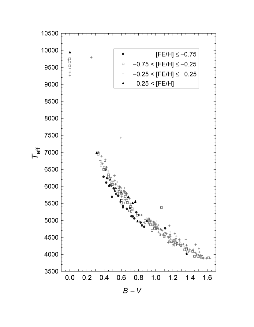
Figure 3: $T_{\rm eff}$ as a function of $B-V$ for the full sample. Different symbols are used to represent metallicity grouped into 4 classes.

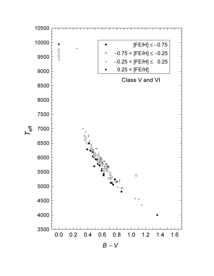
Figure 4: Same as Figure 3, but for dwarfs.

We present in Fig. 3 $T_{\rm eff}$ as a function of unreddened $B-V$ colour for all 283 stars. 13 out of 16 calibrating stars in Table 2 have [Fe/H] and $\log g$ data in SSFRF, and they are also included in the plot. In this figure we classified stars according to metallicity: solid circles are stars with [Fe/H]$\leq-$0.75, open squares for $-0.75<$[Fe/H]$\leq-0.25$, cross symbols for $-0.25<$[Fe/H]$\leq$+0.25, and solid triangles are for [Fe/H]$>$+0.25. The sample covers the range $0.3\leq B-V\leq 1.5$, which is the range of our analysis. In Fig. 4 are selected only dwarfs (and sub-dwarfs). In this sample stars with $B-V>0.9$ are scanty, and we must limit our study to the range between $B-V=0.3$ and 0.9.

In carrying out our fitting, we exclude 17 stars, 10 of them as having $B-V<0.3$, one of them is too distant (700 pc away) and remaining 6 being located more than 4$\sigma$ away from the locus of the fit. Our fitting is made in the following steps. First we fit the samples (full and dwarf samples) simply with $T_{\rm eff}=T_{\rm eff}((B-V)_{0})$ ignoring the [Fe/H] and $\log g$ dependence; we find the rms residual of the fit to be 123K for the full sample and 151 K for the dwarfs. We then carry out a fit with the form

$$\log T_{eff}=c_{0}+c_{1}(B-V)_{0}+c_{2}(B-V)_{0}^{2}+c_{3}(B-V)_{0}^{3}+f_{1}{\rm[Fe/H]}+f_{2}{\rm[Fe/H]}^{2}+g_{1}\log g.$$ (2)

with an equal weight given to all data points. This largely reduces the rms of residuals. We find 66 K (1.1%) for the full sample and 71 K (1.2%) for dwarfs. This rms is somewhat smaller than that of BL98 (80$-$90 K), and smaller by a factor of two than is given by Alonso et al. (1996b) (130 K). In fitting the dwarf sample, we fixed $\log g$ to be constant ($\log g=4.3$) (see below), and $g_{1}$ to the value derived from the fit to the full sample, since the variation of $\log g$ for main sequence stars in this colour range is too small to constrain the fit. The parameters of this fit are given in Table 3. Although we have a strong correlation among coefficients $c_{0}-c_{3}$, and between $f_{1}$ and $f_{2}$, cross correlations are quite small ($<0.1$ when diagonals are normalized to unity) between $c_{i}$ and $f_{j}$. Cross correlations between $c_{i}$ and $g_{1}$, and between $f_{i}$ and $g_{1}$ are also small ($<0.25$ and $<0.15$, respectively). The fit is well constrained expect for a high temperature range $\log T>3.82$: the adoption of variables $T$ or $1/T$ in the right hand of equation (2) does not modify the shape of the curve and the quality of the fit, except at the weakly constrained very end of the high temperature edge where we see a change equivalent to $B-V\leq 0.01$. The parameters for the dwarf sample are consistent with those for the full sample, though the former set has larger errors. The consistency of the two fits means that the two samples are well controlled by simply different $\log g$. Hence, we adopt the fit with the full sample as our best result and use this for further analysis in what follows including that for dwarfs.

We further proceed with our fitting tests. We fit our samples with adding a cross term [Fe/H] $\times$ (B-V)₀. This does not reduces rms residuals at all, but merely increase the error estimate of the parameters (in particular this doubles the error of $f_{1}$), indicating that the cross term is not very well determined. Actually the cross term thus obtained is rather small, and it changes $\partial T_{\rm eff}/\partial$ [Fe/H] only by 14% between $(B-V)=0.4$ and 0.8. So we can drop this term.

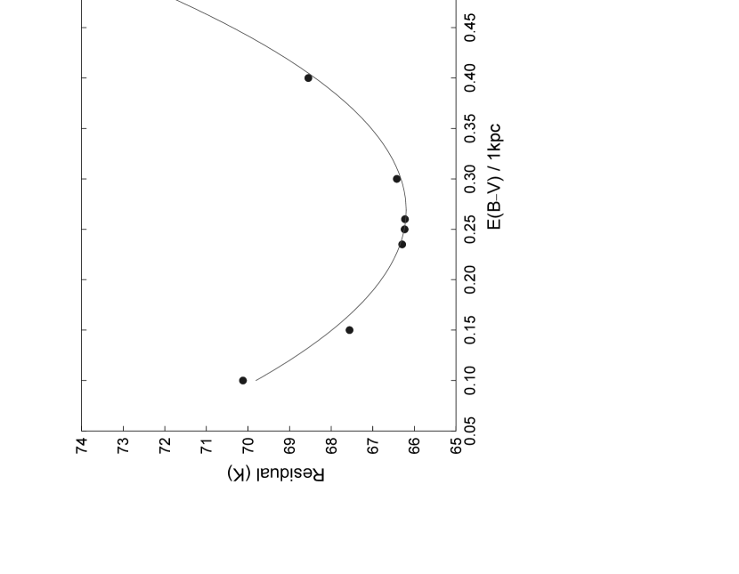
Figure 5: Residual temperature of the fit as a function of the selective extinction per unit distance. The curve is an interpolation.

The next is a fit ignoring extinction corrections. This raises the residual temperature from 66 K to 73 K, indicating the necessity of extinction corrections. The significance is demonstrated in Fig. 5, where we plot the residual rms as a function of the selective extinction per unit distance. We see that the minimum is attained with $E(B-V)=0.269$/kpc, and our adopted value 0.235 increases a residual only less than 0.2 K . We obtain an error of 0.030/kpc for this parameter when this is allowed to vary as a free parameter. This gives not only an excellent confirmation of the selective extinction per distance used in the literature (e.g. Blackwell et al. 1990), but also shows that our fit would differentiate such a small changes in the data, indicating an overall consistency of the fitting procedures.

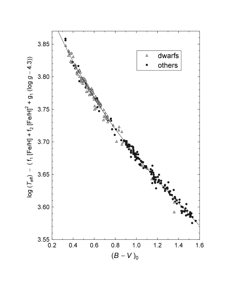
Figure 6: Quality of the fit. The deviation of temperature from the fit is shown for each stars after subtracting expected metallicity contribution and scaled to $\log g=4.3$. Open triangles represent dwarfs and solid circles giants.

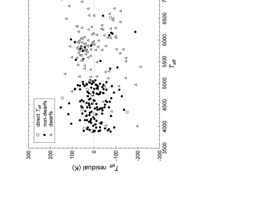
Figure 7: Residual of the fit derived from Fig. 6. Open triangles represent dwarfs and solid circles giants. The stars for which direct temperature measurement are available are plotted with open squares (median value of the data shown in Fig. 2).

The overall quality of our best fit is shown in Fig. 6, where the effective temperature data are corrected for metallicity and surface gravity according to $T_{eff}-(f_{1}{\rm[Fe/H]}+f_{2}{\rm[Fe/H]}^{2}+g_{1}\log g)$, and those points plotted are supposed to give data for [Fe/H]=0 and $\log g$=4.3 as a function of $(B-V)_{0}$. Fig. 7 shows residuals in more detail, where we see that giants and dwarfs are indeed on the same family simply with different $\log g$. This would justify to use the same family of curves for the entire range of our colour space. The data points with squares are stars used for examination of temperature above (we plot only medians when a number of bolometric flux estimates are available).

2.6 Error budget

We have already discussed the source of errors. Our estimate of the size of errors is summarized in Table 4 for F5, G2 and K5 stars. The sources we discussed above all contribute to the dispersion of the final fit. The quadrature of internal error budget amounts to 67$-$77 K, which is consistent with the actual dispersion of the fit 60$-$80 K (global value is 66 K). This means that the error propagation is well controlled in our data processing procedures, and intrinsic scatter of the $(B-V)$ colour temperature relation is substantially smaller than $\approx$40 K.

We note that the error of [Fe/H] and that of $T_{\rm eff}$ are comparable and are the dominant source of errors. Photometry error might compete with this for early type stars, where the curve gets steeper. Errors from other entries are smaller. This dispersion of temperature corresponds to $\delta(B-V)\simeq 0.02$ and increases to 0.03 for low temperature stars. Of course, the locus of the relation is better determined. We anticipate a systematic error up to about 30-40 K in the B98 temperature estimate, and the normalisation error of the bolometric flux, which is used as an external calibrator in our work, of the order of 1.5% (0.37% in temperature), and there may be a systematic trend of metallicity scale on the order of 0.05 dex depending on authors. This makes overall systematic error to be about 45 K (these systematic errors are significantly smaller than the random errors, and are supposed to be already included in the error budget shown in Table 4). This seems to be the best we can achieve with the present data.

3 Comparison of the $B-V/T_{\rm eff}$ relations in the literature

3.1 Dwarfs

We discuss the $B-V$ colour temperature relations ($B-V/T_{\rm eff}$ relations) available in the literature, taking the one we obtained above as a reference. Fig. 8 is a compilation of the colour temperature relations for the main sequence stars with solar metallicity. To draw the locus of our colour temperature relation we assume $\log g=129.34-64.66\log T+8.347(\log T)^{2}$, which is obtained by fitting data of SSFRF for dwarfs used in our analysis. This relation differs from what would be obtained by fitting the data from binary stars (Popper 1980) by an amount of $\Delta\log g\simeq 0.2$ for G stars, but the scatter indicated by the B98 sample (with SSFRF data for $\log g$) and that by the data of Andersen (1991) are somewhat larger than the offset. In any case, the difference caused by the difference of $\log g$ of this amount is small and it changes the resulting temperature by no more than $\approx$ 10 K, or $B-V$ by 0.005.

Now, in order to examine the detail, we display in Fig. 9 the difference of various relations against the one obtained by Lejeune, Cuisinier & Buser (1998; hereafter LCB): $\Delta(B-V)=(B-V)_{0}-(B-V)_{\rm 0,LCB}$. The adoption of their relation as a fiducial zero point is motivated by the fact that their relation covers the widest $B-V$ range, while the range of the relation we obtained is not as wide as theirs. In this figure we have plotted 9 relations, which we are going to discuss in detail: Flower (1996), Alonso et al. (1996b), BL98, Code et al. (1976), Demarque et al. (1985; Yale isochrone), and Bertelli et al. (1994), and the relation derived using ATLAS9 (Kurucz 1993) atmosphere, together with LCB and ours. The Yale isochrone and Bertelli et al. are theoretical estimates based on model atmospheres, and we have computed colours for ATLAS9 using the response functions of Azusienis and Straizys (1969) for the $B$ and $V$ pass bands. Table 4 summarizes briefly the methods adopted by the respective authors. We also plot the position of the sun taking ($T_{\rm eff}=5777\pm 6$ K and $B-V=0.64\pm 0.01$, which we discuss in the next section.

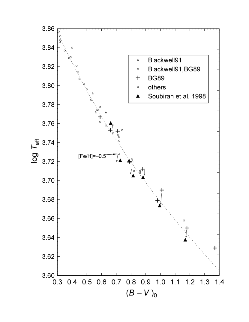
Figure 10: The data points for $B-V$ colour temperature relation used by Flower (1996), overlayed with new determination of the temperature for the same stars (when available), the change indicated by arrows. One point with given metallicity is star largely deviated from solar. The dotted curve is the $B-V$ colour temperature relation given in eq. (2). BG89 stands for Bell & Gustafsson (1989).

It is clear at a glance that LCB and Flower (1996) are largely deviated from the others including our newly obtained $B-V/T_{\rm eff}$ relation. Flower uses temperature information collected from various sources: some from direct measurements of angular diameters, some from IRFMs, and others from spectroscopic analysis. For $\log T_{\rm eff}<3.75$, where a large departure starts, Flower’s data mostly rely on temperature from an IRFM analysis of Bell & Gustafsson (1989). To study a possible problem with Flower’s temperature, we show in Fig. 10 the stars he used. In the range of our interest $B-V>0.65$, we find new temperature determinations by Soubiran, Katz & Cayrel (1998) for 7 stars (indicated by arrows). The new temperature for these stars are significantly lower as we go to redder stars, and they fall on the curve of $B-V/T_{\rm eff}$, we have obtained in this paper. This lends an additional support for our $B-V/T_{\rm eff}$, and at the same time indicates that temperature obtained with the Bell & Gustafsson atmosphere suffers from errors for stars later than the G5 type ($T_{\rm eff}<5500$ K). Flower’s relation reflects this overestimate of temperature for late type stars.

LCB adopts Flower’s $B-V/T_{\rm eff}$ for $T_{\rm eff}>4250$ K (log $T_{\rm eff}>3.63$), so that it is identical with Flower’s for this temperature range. Accordingly, LCB’s $B-V/T_{\rm eff}$ relation inherits the same problem as Flower’s.

BL98 agree with ours for a rather wide range $3.68<\log T_{\rm eff}<3.78$ to within 0.02 mag. Beyond $3.78<\log T_{\rm eff}$ (6000 K) BL98 shows a sudden break and turns away from our curve, giving significantly bluer colour; At log $T_{\rm eff}>3.80$ it is bluer by 0.04 mag than ours. B98 examined his surface brightness against IRFM of BL98 for the main-sequence stars and found that BL98 give angular diameter larger by 4% at log($T_{\rm eff}$)=3.95, while there is no offset between the two at log($T_{\rm eff}$)=3.72. This 4% offset is consistent with BL98’s $B-V$ bluer by 0.03-0.04 mag than ours.

Alonso et al (1996b)’s $B-V/T_{\rm eff}$ relation, which is based on IRFM with ATLAS9 atmosphere supplemented with a calibration against angular diameter measurements, is closely parallel to ours. The agreement between the two is $<0.01$ mag in $B-V$ for 3.75$<$log($T_{\rm eff}$)$<$3.85. The difference gradually increases as temperature decreases, and it becomes 0.03 mag at the end point of Alonso et al., log($T_{\rm eff}$)=3.70.

We have retained in Fig. 9 old Code et al. (1976)’s $B-V/T_{\rm eff}$ relation, which is based on a direct angular size measurement employing intensity interferometry. Their curve smoothly matches with ours with the difference is no more than 0.01 mag in the overlapping range 3.76$<$log($T_{\rm eff}$)$<$3.85.

Our final assessment concerns the theoretical colour temperature relations used by the Yale isochrone (Demarque et al. 1996) and by Bertelli et al. (1994), and the one derived from ATLAS9. The departure from our empirical $B-V/T_{\rm eff}$ relation is significant, and the difference can be 0.04 mag. The discrepancy is even larger with the $B-V/T_{\rm eff}$ relation derived from the Kurucz (1991, unpublished) atmosphere (Bertelli et al. 1994): at log($T_{\rm eff}$)=3.75, it gives 0.05 mag redder than our relation. It is interesting to note that these theoretical $B-V/T_{\rm eff}$ relations give values in agreement with ours at log($T_{\rm eff}$)=3.65. This implies that the theoretical relations, if they are used to connect K5 stars with G5 stars, raise systematic errors of 0.04 to 0.05 mag for relative colours of stars between these two types. When translated into $M_{V}$, this systematic offset amounts to 0.24-0.30 mag for a given $B-V$. We see the same trend with the calculation using ATLAS9 (Kurucz 1993) atmosphere, although it shows larger deviations at both lower and higher temperatures from ours than the curve of Bertelli et al. who used 1991 version of Kurucz’ atmosphere.

3.2 Giants

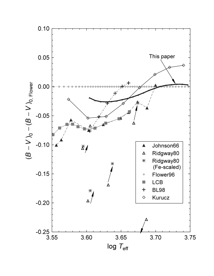
Figure 11: Comparison of the $B-V$ colour temperature relations for giants. The relation of Flower (1996), which covers the widest range, is taken as the zero point. The arrows show the metallicity correction applied to the data points by Ridgway et al. (1980).

A similar analysis is carried out for giants. We have plotted $\Delta(B-V)=(B-V)_{0}-(B-V)_{\rm 0,Flower}$ in Fig. 11, taking this time Flower’s (1996) relation that covers the widest range as the zero point. The figure includes classical work by Johnson (1966) and Ridgway et al. (1980), which have been taken as the standard for long, and recent work by LCB and BL98; a synthetic calculation using theoretical atmosphere of Kurucz (1993) is also included. As for Ridgway et al. (1980)’s data points, we assign $B-V$ colours from Hauck & Mermilliod (1998) for the stars they used. Since the scatter is to large to obtain a sensible fit, however, we instead plot the points of individual stars. We have also indicated the metallicity correction, when [Fe/H] data are available, by arrows using the metallicity gradient given in eq. (2).

It is seen in Fig. 11 that Johnson (1966) and LCB are 0.03$-$0.04 mag bluer than our $B-V/T_{\rm eff}$ relation for a $T=4000-4500$ K range, and Flower (1996) are 0.03$-$0.04 redder in the same range. Unfortunately, our formula does not reliably apply to the temperature lower than 4000 K. BL98 give a $B-V/T_{\rm eff}$ relation with slope somewhat steeper than ours, and the disagreement increases to $>$0.3 mag for $T<4300$ K ($\log T<3.63$). Ridgway et al.’s data are too noisy to make an accurate comparison, but it is likely that their colour temperature relation, when transformed to the $B-V$ colour band, giving too blue colours, say by 0.10$-$0.15 mag for K giants (see also Flower 1996).

A good agreement ($\Delta(B-V)<0.02$ mag) is seen between our curve and Kurucz (1993) for a range 4200 K (the lowest temperature) and 5100 K. Kurucz (1993) gives redder colours only for giants earlier than G type.

4 Colour of the Sun

$B-V$ colour of the sun has been playing an important role as a normalization point for the stellar evolution models, yet observationally an accurate measurement of solar colours is notoriously difficult. Photometric observations yield 0.63 (Stebbins & Kron 1957) to 0.69 (Tüg & Schmidt-Kaler 1982). The method often adopted by observers is to use observations of other stars, and interpolate and translate them to the sun, which typically leads to 0.633$\pm$0.009 or 0.665$\pm$0.003 (Taylor 1998), or look for “solar twins” (de Strobel 1996, for a summary), rather than to work directly with the sun. For this solar analogue method to work properly, it is essential to control the accuracy of temperature and also metallicity of these stars; this is not easy a task, as we have seen in the preceding section.

In Fig. 9 the zero point at $T_{\rm eff}=5777$ K is adjusted to LCB’s value $B-V=0.633$. Our compilation shows that all modern determinations of the $B-V/T_{\rm eff}$ relation give colours equal to or about 0.1 mag bluer than this value. In particular, our newly obtained curve gives $B-V=0.627$. The bluest value is given by Alonso et al. (1996b)’s curve, which yields 0.621. On the other hand, synthetic colors from atmosphere models are significantly redder, 0.65 with the colour-temperature relation of the Yale isochrone, and 0.67 with Kurucz’ atmosphere (Bertelli et al 1994; Bessell, Castelli and Plez 1998).

Many solar analogue analyses in the past gave rather redder colour, such as 0.66 (e.g., Hardrop 1978; Wamstecker 1981). de Strobel (1996) has argued that Hardrop’s sample is significantly metal rich, leading to redder colour. This is also true with, e.g., Wamstecker’s sample. The stars in his sample have either luminosity lower than the sun or metallicity higher than the sun by +0.15 dex. After careful selection de Strobel concluded that $B-V=0.642\pm 0.004$.

Here we re-examine the case with de Strobel (1996)’s analysis in view of our assessment for the temperature estimate. She has given 26 stars on the list of effective-temperature-selected solar analogues. Among those stars 8 stars are given temperature by B98, and BL98’s temperature estimate is available for additional two stars (at the solar temperature, BL98 and B98 agree very well). For 6 stars among these 10 stars, de Strobel has given temperature based on spectroscopic studies much higher than BL98 and B98; the difference amounts to 100-160 K. The average of the offset in the two $T_{\rm eff}$ estimates amounts to 63 K with de Strobel’s temperature higher. The adjustment of temperature can easily modify de Strobel’s estimate of $(B-V)_{\odot}$ into a bluer value by an amount of 0.02 or so.

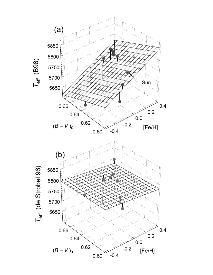
Figure 12: (a) Solar analogue stars of de Strobel (1996) selected on the basis of temperature in $T_{\rm eff}$, $(B-V)_{0}$, [Fe/H] space. Only those stars that have B98 temperature estimates are plotted, and temperature is taken from B98. The plane shows a bilinear fit, and line segment attached to data are distances from the plane. (b) Same as (a) but with the temperature given by de Strobel.

We have tried to find solar colour by fitting the 8 stars with B98 data to the form $T_{\rm eff}=c_{0}+c_{1}(B-V)+f_{1}[{\rm Fe/H}]$ using the B98 temperature data. In spite of a small sample and a small range, the fit is well constrained, yielding $(B-V)_{\odot}=0.61$, with metallicity gradient $\partial T_{\rm eff}/\partial{\rm[Fe/H]}=$ 220 K/dex and temperature gradient of the right order of magnitude, although this temperature-selected sample is clearly too narrow in the temperature range to find the correct gradient (see Fig. 12a). When we replace the B98 temperature with de Strobel’s ([Fe/H] data are not replaced), however, we obtain the temperature basically constant at 5820 K and metallicity gradient with the sign opposite to what we have obtained with the B98 temperature (Fig. 12b). This indicates that the spectroscopic temperature does not agree with the bolometry-surface brightness estimate we used in this paper. This uncertainty in temperature estimations tells us a difficulty of an accurate estimate of solar colour from solar analogues: one must know star’s temperature to an absolute accuracy of $\pm 50$ K and [Fe/H]$<$ 0.1. The former is the accuracy one can barely achievable with the bolometry-surface brightness estimate as we have seen in this paper.

From our $B-V/T_{\rm eff}$ relation we conclude $(B-V)_{\odot}=0.627\pm 0.014\pm 0.012$ with the two errors standing for uncertainty of the estimate of the locus of the relation and possible intrinsic dispersion for the sun around the relation. All modern $B-V/T_{\rm eff}$ relations (other than synthetic) documented in Fig. 9 give $(B-V)_{\odot}$ within this error. We are not able to reconcile our value with a red colour 0.66-0.67, often referred to in the literature. If the sun would really be this red, it is significantly off from normal G2 stars.

Our final remark concerns colour of the sun from spectroscopic synthesis that synthesis calculations using the measured solar spectrum tend to give bluer colours 0.61-0.65 (see Fukugita, Ichikawa & Sekiguchi 1999 for details), and this agrees with the value we have inferred above.

5 Metallicity dependence

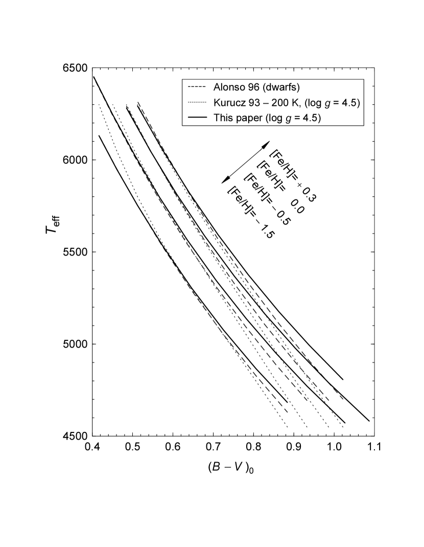
Figure 13: Metallicity dependence of the $B-V$ colour temperature relation for dwarfs. The curves are plotted for [Fe/H]=$-1.5,-0.5,0$ and +0.3. The curves derived from Kurucz atmosphere are shifted downward by 200 K to ease a comparison.

We present the metallicity dependence of our $B-V/T_{\rm eff}$ relation in Fig. 13. Three solid curves represent the relations for [Fe/H]=$-$1.5, $-$0.5, 0 and 0.3 for main sequence. We limit our plot to $0.3<B-V<1.0$, for which our metallicity dependence is well constrained by data. We overlay the curves of Alonso et al. (1996b) and the one we computed with Kurucz (1993) atmosphere, where Kurucz’ temperature is scaled down by 200 K to make figure ease a comparison in the same figure.

With our curve $\partial T_{\rm eff}/\partial{\rm[Fe/H]}=325\pm 20$ K/dex, owing to the absence of a [Fe/H]*$(B-V)$ term as discussed in section 2.5. This means for G2 stars $\partial(B-V)/\partial[{\rm Fe/H}]=0.9$ mag/dex for the portion contributed from the atmosphere. If we adopt the fit where the cross term is taken as a free parameter the partial derivative increases towards bluer side by 50 degree between $B-V=0.8$ and 0.4.

Apparently a good gross agreement is seen between Alonso et al. and ours. A more careful examination, however, shows that metallicity gradient of the former increases from 330 K/dex at $B-V=0.8$ to 480 K/dex at 0.4. We have not seen this large change with our fit, even if we allow for the cross term: our analysis shows that it is at most one third this value.

The family of curves calculated with Kurucz (1993)’s atmosphere is generally shifted by about 200 K to a lower temperature. With shifting by this amount, the curve derived from Kurucz’s atmosphere agrees well with ours for the range $0.5<B-V<0.7$. On the other hand, the metallicity gradient shows a very good agreement with ours: $\partial(B-V)/\partial{\rm[Fe/H]}$ stays between 350$-$370 K/dex in the range $B-V=0.4-0.8$ with the Kurucz atmosphere. The metal dependence is well accounted for with the Kurucz atmosphere for F-K stars.

6 Conclusion

In this paper we have used the modern, least model-dependent determination of effective temperature of stars and the best available data for $B-V$ colours, metallicity and surface gravity in order to derive a $B-V$ colour temperature relation with metallicity and gravity as auxiliary parameters. We have achieved the smallest residual temperature over those available in the literature. The fit we obtained is well constrained and a number of tests assure the quality of data and show a consistency of the data processing procedures. Our relation covers the range from F0 to K5 stars ($T_{\rm eff}=4000-7000$ K) and [Fe/H] from $-$1.5 to +0.3 both for dwarfs and giants. The dispersion of the fit, 66 K, perhaps represents the limit we can achieve with the present quality of data.

The most important limiting factors are temperature determinations and metallicity measurements. This means that we can attain accuracy of 0.02 mag in $B-V$ colours for a given temperature for F0-K0 stars, and slightly worse for later type stars. This is still a significant error, but it is not as large as the disagreement recognized among various isochrone works.

We have examined various $B-V/T_{\rm eff}$ relations available in the literature. Our relation smoothly joins the Code et al. (1976)’s relation given for high temperature stars, and also shows a close match with Alonso et al. (1996b)’s $B-V/T_{\rm eff}$ relation which is based on the IRFM with additional calibrations. BL98 give a relation that agrees reasonably well with ours, but a significant discrepancy is observed for stars earlier than F8 stars. The relations of Flower (1996) and LCB are largely off from ours, as much as 0.1 mag for low temperature stars. Colour becomes significantly redder for G5 or later type stars, if these $B-V/T_{\rm eff}$ relations are used. Our comparison demonstrates that some calibration of temperatures against those obtained from angular diameter measurements consists an essential element for a high accuracy.

We also clarified systematic errors with the colour-temperature relation obtained by synthetic computation using model atmospheres: they deviate significantly from our empirical relation. In particular, the offset changes by 0.04-0.05 in $B-V$ across K0 to K5 stars, which directly induces an error in the slope of the colour-magnitude diagram by this amount. This means that, for instance, if the distance to one open cluster is calibrated with K5 stars and if another is with K0 or some earlier stars, we would be led to an error of 10-15% in distance. This error also makes intermediate age galaxies, which contains G stars as a major source of the bluer component, appreciably redder in stellar population synthesis model of galaxies.

Another implication important for cosmology is that the population synthesis model of Bruzual & Charlot (1993) (see also Charlot, Worthey & Bressan 1996) would give too blue colour for early type galaxies in their late stage of evolution. Typically 5 Gyr after the initial burst, G and K giants start dominating the light from elliptical galaxies, and Bruzual & Charlot take Ridgway et al (1980)’s temperature scale to assign colours to tracks. We have shown that Ridgway et al.’s scale gives typically 0.1 mag bluer at a given temperature for K giants. Therefore, we should make Bruzual & Charlot’s $B-V$ colour prediction redder by this amount. With this revision, the burst model would give $B-V=0.95$ already at 5 Gyr from the burst, rather than 9 Gyr in their original model. This offset also explains the discrepancy, at least in part, between the predictions of Bruzual & Charlot and of Bertelli et al. (1994), the latter, using the Kurucz atmosphere, giving 0.05 magnitude redder than the former.

We have also studied the problem of colour of the sun. Our $B-V/T_{\rm eff}$ relation gives $(B-V)_{\odot}=0.63\pm 0.02$ which agrees with “long wavelength group”, but disagree with “short wavelength group” of solar colour (Taylor 1998). We have emphasized the importance to accurately estimate temperature and metallicity when colour of the sun is inferred from solar analogues. The quality of temperature and metallicity determinations of the presently available sample is probably insufficient to determine colour of the sun within an error of 0.02 mag.

Table 1: Colour temperature relation and derivatives

$B-V$	$T_{\rm eff}$	${\partial T_{eff}\over\partial(B-V)}\times 10^{-2}$
0.3	7078	$-$48
0.4	6621	$-$43
0.5	6214	$-$38
0.6	5852	$-$34
0.7	5532	$-$30
0.8	5248	$-$27
0.9	4996	$-$24
1.0	4770	$-$21
1.1	4567	$-$19
1.2	4382	$-$18
1.3	4209	$-$17
1.4	4044	$-$16
1.5	3882	$-$16

Table 2: Data for the temperature check

BS	LC	$\phi$	$(V-K)_{0}$	$F_{\rm bol}$	ref/norm	$T_{\rm eff}$(ref)	$\Delta T_{\rm eff}$(B98)	$T_{\rm eff}$(BL98)
		(mas)		($10^{-6}$erg cm-2s-1)		(K)	(K)	(K)
2491	V	5.92$\pm$.09	-.099	114.3$\pm$4.4	a/A	9947$\pm$122	$-$3
7001	V	3.24$\pm$.07	$-$.001	30.4$\pm$1.2	a/A	9655$\pm$141	$-$184
7001	V	3.24$\pm$.07	$-$.001	29.0$\pm$2.6	b/B	9542$\pm$237	$-$71
6879	V	1.44$\pm$.06	.047	5.53$\pm$0.22	a/A	9458$\pm$218	$-$203
4534	V	1.33$\pm$.10	.140	3.61$\pm$0.13	a/A	8847$\pm$342	16
8728	V	2.10$\pm$.14	.144	8.80$\pm$0.31	a/A	8797$\pm$303	50	8622$\pm$86
6556	III	1.63$\pm$.13	.379	3.65$\pm$0.13	a/A	8013$\pm$327	$-$16	7883$\pm$63
6556	III	1.63$\pm$.13	.379	3.640$\pm$0.218	b/B	8008$\pm$341	$-$10	7883$\pm$63
2943	IV.5	5.51$\pm$.05	1.010	18.08$\pm$0.76	a/A	6502$\pm$74	56
2943	IV.5	5.51$\pm$.05	1.010	18.35$\pm$0.367	c/C	6526$\pm$44	32
Sun	V	19193E2	1.486	1.370(2)E+12	d/D	5780$\pm$2	$-$16
2990	III	8.04$\pm$.08	2.246	11.82$\pm$0.47	e/E	4840$\pm$54	$-$45	4837$\pm$29
2990	III	8.04$\pm$.08	2.246	11.78$\pm$0.12	f/A+B	4836$\pm$27	$-$41	4837$\pm$29
2990	III	8.04$\pm$.08	2.246	11.69$\pm$0.47	g/F	4827$\pm$54	$-$31	4837$\pm$29
7949	III	4.62$\pm$.04	2.398	3.598$\pm$0.036	f/A+B	4743$\pm$24	$-$88	4732$\pm$28
168	III	5.64$\pm$.05	2.430	5.00$\pm$0.15	h/	4660$\pm$41	$-$34
617	III	6.85$\pm$.06	2.630	6.43$\pm$0.20	h/	4503$\pm$40	$-$42
165	III	4.12$\pm$.04	2.853	2.105$\pm$0.021	f/A+B	4392$\pm$24	$-$93	4335$\pm$30
5340	III	20.95$\pm$.20	2.921	49.21$\pm$0.49	f/A+B	4283$\pm$23	$-$28
5340	III	21.00$\pm$.20	2.921	49.21$\pm$0.49	f/A+B	4278$\pm$23	$-$23
5340	III	20.95$\pm$.20	2.921	49.77$\pm$0.10	g/F	4295$\pm$30	$-$41
5340	III	21.00$\pm$.20	2.921	49.77$\pm$0.10	g/F	4290$\pm$30	$-$35
6705	III	10.13$\pm$.24	3.503	8.408$\pm$0.084	f/A+B	3960$\pm$48	$-$20
6705	III	10.20$\pm$.20	3.503	8.408$\pm$0.084	f/A+B	3946$\pm$40	$-$6
6705	III	10.13$\pm$.24	3.503	8.330$\pm$0.417	b/B	3951$\pm$68	$-$10
6705	III	10.20$\pm$.20	3.503	8.330$\pm$0.417	b/B	3937$\pm$63	3
6705	III	10.13$\pm$.24	3.503	8.59$\pm$0.34	g/F	3981$\pm$61	$-$41
6705	III	10.20$\pm$.20	3.503	8.59$\pm$0.34	g/F	3968$\pm$55	$-$27
1457	III	20.88$\pm$.10	3.704	33.49$\pm$0.335	f/A+B	3897$\pm$13	$-$37
1457	III	21.21$\pm$.21	3.704	33.49$\pm$0.335	f/A+B	3866$\pm$21	$-$7
1457	III	20.88$\pm$.10	3.704	33.82$\pm$1.35	g/F	3906$\pm$40	$-$47
1457	III	21.21$\pm$.21	3.704	33.82$\pm$1.35	g/F	3876$\pm$43	$-$16

References. — (a) Code et al. (1976), (b) Leggett et al. (1986), (c) Alosno et al. (1995), (d) Bahcall & Pinsonneault (1995), (e) Blackwell & Lynas-Grey (1994), (f) Blackwell et al. (1990), (g) Di Benedetto & Rabbia (1987), (h) Faucherre et al. (1983), (A) $3.36\times 10^{-9}$ (erg cm^-2s^-1) at 5556Å   Oke & Schild (1970); (B) $3.39\times 10^{-9}$ (erg cm^-2s^-1) Hayes & Latham (1975) (C) $3.47\times 10^{-9}$ (erg cm^-2s^-1) Tüg, White & Lockwood (1977); (D) ; (E) $3.45\times 10^{-9}$ (erg cm^-2s^-1) Dreiling & Bell (1980); (F) $3.42\times 10^{-9}$ (erg cm^-2s^-1) Hayes (1979)

Table 3: Fit parameters

	full sample	main sequence
range	0.3$<B-V_{0}<$1.5	0.3$<B-V_{0}<$0.9
data points	266	104
$c_{0}$	3.98319 $\pm$ 0.00727	3.97542 $\pm$ 0.01441
$c_{1}$	$-$0.42998 $\pm$ 0.02630	$-$0.40671 $\pm$ 0.06180
$c_{2}$	0.18174 $\pm$ 0.02999	0.16881 $\pm$ 0.08292
$c_{3}$	$-$0.04280 $\pm$ 0.01050	$-$0.04830 $\pm$ 0.03413
$f_{1}$	0.02691 $\pm$ 0.00173	0.02576 $\pm$ 0.00234
$f_{2}$	0.00437 $\pm$ 0.00100	0.00454 $\pm$ 0.00128
$g_{1}$	$-$0.003223 $\pm$ 0.000648	$-$0.003223 (fixed)

Table 4: Summary of estimated errors (dispersion)

source	error	$\Delta T_{\rm eff}$(F5)	$\Delta T_{\rm eff}$(G2)	$\Delta T_{\rm eff}$(K5)
$T$		6500	5800	4500
$\Delta T$		40	40	40
$\Delta(B-V)$	0.01	41	33	18
$\Delta E(B-V)$	0.003	14	11	6
$\Delta{\rm[Fe/H]}$	0.15	50	50	50
$\Delta\log g$	0.2	6	6	6
quadrature sum		77	73	67
$\sigma$ of the fit		80	66	60

Table 5: Literature appeared in Figs. 8 and 9

legend	reference : method : range
Code76	Code et al. 1976 : $\phi$ (interferometry) and $F_{\rm bol}$ : $T_{\rm eff}>5780K$, LC=V
VB85	VandenBerg & Bell 1985 : Bell & Gustafsson 1978 atmosphere
Bertelli94	Bertelli et al. 1994 : Kurucz 1993 atmosphere for $T_{\rm eff}>4000$K
Yale96	Demarque et al. 1996 : model atmosphere
Flower96	Flower 1996 : compilation of $T_{\rm eff}$ : LC=V-III and II
Alonso96	Alonso et al. 1996 : IRFM (Kurucz 1991, 1993) : $0.2<B-V<1.5$, LC=V
LCB	Lejeune et al. 1997 : used Flower 1996 for $T_{\rm eff}>4250$K:
	$\log g$ and [Fe/H] extension with Kurucz atmosphere
BL98	Blackwell & Lynas-Gray 1998 : IRFM (Kurucz 1992): 4000$<T_{\rm eff}<$9000K, LC=V,IV,III

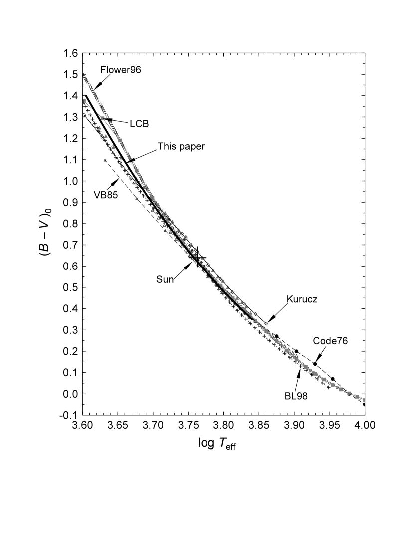
Figure 8: Compilation of $B-V$ colour temperature relations for dwarfs available in the literature, as compared with the one obtained in this paper. The relation is given for the solar abundance.

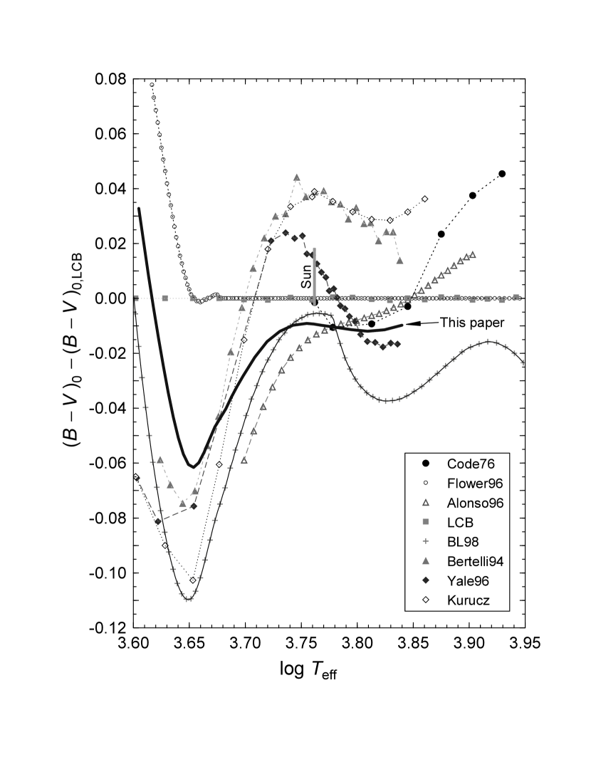
Figure 9: Comparison of $B-V$ colour temperature relations for dwarfs. The difference is plotted for various $B-V$ colour temperature relations, taking the one by LCB, which covers the widest parameter range as the zero point. All relations are plotted at solar metallicity. The position of the sun with $B-V=0.64\pm 0.01$ and $T_{\rm eff}$=5777 K is also shown. For legends see Table 5.

References

- (1)
- (2) Alonso, A., Arribas, S. & Martínez-Roger, C. 1995, A&A, 297, 197
- (3)
- (4) Alonso, A., Arribas, S. & Martínez-Roger, C. 1996a, A&AS, 117, 227
- (5)
- (6) Alonso, A., Arribas, S. & Martínez-Roger, C. 1996b, A&A, 313, 873
- (7)
- (8) Andersen, J. 1991, ARA&A, 3, 91
- (9)
- (10) Arribas, S. & Martínez-Roger, C. 1988 A&A, 206, 63
- (11)
- (12) Azusienis, A. & Straizys, V. 1969, AZ, 13, 316
- (13)
- (14) Bahcall, J. N. & Pinsonneault, M. H. 1995, Rev Mod Phys, 67, 781
- (15)
- (16) Bell, R. A. & Gustafsson, B. 1989, MNRAS, 236, 653
- (17)
- (18) Bertelli, G., Bressan, A., Chiosi, C., Fagotto, F. & Nasi, E. 1994, A&AS, 106, 275
- (19)
- (20) Bessell, M. S. 1979, PASP, 91, 589
- (21)
- (22) Bessell, M. S., Castelli, F. & Plez, B. 1998, A&A, 333, 231
- (23)
- (24) Blackwell, D. E. & Lynas-Gray, A. E. 1994, A&A, 282, 899
- (25)
- (26) Blackwell, D. E. & Lynas-Gray, A. E. 1998, A&AS, 129, 505 (BL98)
- (27)
- (28) Blackwell, D. E., Lynas-Gray, A. E. & Petford, A. D. 1991, A&A, 245, 567
- (29)
- (30) Blackwell, D. E., Petford, A. D., Arribas, S., Haddock, D. J., Selby, M. J. 1990, A&A, 232, 396
- (31)
- (32) Blackwell, D. E. & Shallis, M. J. 1977, MNRAS, 180, 177
- (33)
- (34) Böhm-Vitense, E. 1980, ARA&A, 19, 295
- (35)
- (36) Bruzual A, G. & Charlot, S. 1993, ApJ, 405, 538
- (37)
- (38) Charlot, S., Worthey, G. & Bressan, A. 1996, ApJ, 457, 625
- (39)
- (40) Code, A. D., Davis, J., Bless, R. C. & Hanbury-Brown, R. 1976, ApJ, 203, 417
- (41)
- (42) Davis, J. 1998, in Fundamental Stellar Properties, ed. T. R. Bedding et al. (Dordrecht, Kluwer), p. 31
- (43)
- (44) Demarque, P., Chaboyer, B., Guenther, D., Pinsonneault, M, Pinsonneault, L., & Yi, S. 1996, Yale Isochrones
- (45)
- (46) de Strobel, G. C. 1996, ARA&A, 7, 243
- (47)
- (48) de Strobel, G. C., Soubiran, C., Friel, E. D., Ralite, N. & Francois, P. 1997, A&AS, 124, 299 (SSFRF)
- (49)
- (50) Di Benedetto, G. P. 1998, A&A, 339, 858 (B98)
- (51)
- (52) Di Benedetto, G.P., Rabbia, Y. 1987, A&A, 188, 114
- (53)
- (54) Dreiling, L. A. & Bell, R. A. 1980, ApJ, 241, 736
- (55)
- (56) ESA 1997, The Hipparcos Catalogue ESA SP-1200
- (57)
- (58) Faucherre, M., Bonneau, D., Koechlin, L. and Vakili, F. 1983, A&A, 120, 263
- (59)
- (60) Flower, P. J. 1996, ApJ, 469, 355
- (61)
- (62) Fukugita, M., Ichikawa, T. & Sekiguchi, M. 1999, in preparation
- (63)
- (64) Gustafsson, B., Bell, R. A., Eriksson, K., Nordlund, Å 1975, A&A, 42, 407
- (65)
- (66) Hardrop, J. 1978, A&A, 63, 383
- (67)
- (68) Hauck, B. & Mermilliod, M. 1998, A&AS, 129, 431
- (69)
- (70) Hayes, D. S. & Latham, D. W. 1975, AJ, 197, 593
- (71)
- (72) Hayes, D. S. 1979, Dudley Obs. Reports, No.14, ed. A.G. Davis Phillips (Dudley Observatory, NY), p. 297
- (73)
- (74) Hayes, D. S. 1985, in Calibration of Fundamental Stellar Quantities, IAU Symposium 111, ed. D. S. Hayes et al. (Dordrecht, Reidel), p. 225
- (75)
- (76) Hayes, D. S. and Latham, D. W. 1975, ApJ, 197, 593
- (77)
- (78) Johnson, H. L. 1966, ARA&A, 4, 193
- (79)
- (80) Kodama, T & Arimoto, N. 1997, A&A, 320, 41
- (81)
- (82) Kurucz, R. L. 1993, Atmosphere models CD-ROM
- (83)
- (84) Leggett, S. K. et al. 1986, A&A, 159, 217
- (85)
- (86) Lejeune, T., Cuisinier, F. & Buser, R. 1998, A&AS, 130, 65 (LCB)
- (87)
- (88) Mégessier, C. 1994, A&A, 289, 202
- (89)
- (90) Mermilliod, J. C., Turon, C., Robichon, N., Arenou, F. & Lebreton, Y. 1997, Proceedings of the ESA Symposium ‘Hipparcos - Venice ’97’, (Noordwijk, ESA), p. 689
- (91)
- (92) Nordström, B., Andersen, J. & Andersen, M. I. 1997, A&A, 322, 460
- (93)
- (94) Oke, J. B. and Schild, R. E. 1970, ApJ, 161, 1015
- (95)
- (96) Pinsonneault, M. H., Stauffer, J., Soderblom, D. R., King, J. R. & Hanson, R. B. 1998, ApJ, 504, 170
- (97)
- (98) Popper, D. M. 1980, ARA&A, 18, 115
- (99)
- (100) Ridgway, S. T., Joyce, R. R., White, N. M. & Wing, R. F. 1980, ApJ, 235, 126
- (101)
- (102) Saxner, M. & Harmmarbäck, L. W. 1985, A&A, 151, 372
- (103)
- (104) Soubiran, C., Katz, D., Cayrel, R. 1998, A&AS, 133, 221
- (105)
- (106) Stebbins, J.& Kron, G. E. 1957, ApJ, 126, 266
- (107)
- (108) Taylor, R. J. 1998, in Fundamental Stellar Properties, ed. T. R. Bedding et al. (Dordrecht, Kluwer), p.83
- (109)
- (110) Tinsley, B. M. & Gunn, J. E. 1976, ApJ, 203, 52
- (111)
- (112) Tsuji, T., Ohnaka, K., Aoki, W. & Nakajima, T. 1996, A&A, 308, L29
- (113)
- (114) Tüg, H. & Schmidt-Kaler, T. 1982, A&A, 105, 400
- (115)
- (116) Tüg, H., White, N. M. & Lockwood, G. W. 1977, A&A, 61, 679
- (117)
- (118) VandenBerg, D. A. and Bell, R. A. 1985, ApJS, 61, 531
- (119)
- (120) van Leeuwen, F. 1999, A&A, 341, L71
- (121)
- (122) van Leeuwen F. & Hansen Luiz, C.S. 1997, Proceedings of the ESA Symposium ‘Hipparcos - Venice ’97’ (Noordwjik, ESA) p. 689
- (123)
- (124) Wamstecker, W. 1981, A&A, 97, 329
- (125)