Perturbative analysis in planetary
gravitational lensing

Abstract

The traditional perturbative method is applied to the case of gravitational lensing of planetary systems. A complete and detailed description of the structure of caustics for a system with an arbitrary number of planets can be obtained. I have also found precise analytical expressions for microlensing light curves perturbed by the presence of planets.

1 Introduction

In the last years, the prediction and the observation of many microlensing events are gathering ever more interest in gravitational lensing. The typical light amplification curve for these events, found by Paczynski in 1986, has been observed by several astronomical collaborations in observation campaigns toward the bulge of our galaxy (Udalski et al., 1993a; Alard et al., 1997), the Large Magellanic Cloud and the Small Magellanic Cloud (Alcock et al., 1993; Aubourg et al., 1993), the spiral arms and Andromeda galaxy (Tomaney & Crotts, 1996; Ansari et al., 1997; Melchior et al., 1999). Recently, observations toward globular clusters have even been suggested (Jetzer, Strassle & Wandeler, 1998). Beyond proving the correctness of Paczynski’s predictions, the observation of microlensing events provides a very cunning instrument for the investigation of the halo of our (and/or some other) galaxy.

Together with events strictly following Paczynski’s curve, some events showing deviations from the standard behaviour have been detected. Each of these deviations has found some interpretation (Finite source cut-off (Witt & Mao, 1994; Alcock et al., 1998), blending (Sutherland, 1998), parallax effect (Gould, 1992; Alcock et al., 1995), binary lens (Schneider & Weiss, 1986; Mao & Paczynski, 1991; Udalski et al., 1993b). Indeed, the most intriguing of these deviations is the one induced by a binary (or multiple) lens.

The study of light amplification curves produced by multiple lenses has not yet been performed analytically because of the difficulties in the inversion of the lens application. Anyway, these curves can be obtained numerically by using some inversion algorithm (inverse ray shooting)(Wambsganns, 1997). From the analytical point of view, only the caustics of a general binary lens have been studied in some detail (Witt & Petters, 1993). The lack of analytical results utilizable in microlensing constitutes an irksome obstacle in the complete interpretation of multiple microlensing events.

A particularly interesting case of multiple Schwarzschild lenses is formed when one of the masses is much biggest than others (Mao & Paczynski, 1991; Gould & Loeb, 1992). This is the situation of a typical planetary system where a central star is surrounded by its planets bearing masses thousand or million times smaller. The perturbations on Paczynski’s curve induced by the presence of a (even Earth - like) planet are in principle detectable by collaboration teams exploiting world wide telescopic networks (Peale, 1997; Sackett, 1997). Then microlensing could become a new efficient method for the detection of small planets in extra - solar systems. This justifies the major interest in this field that is growing in the last months. Preliminary calculations on the probability of detection of planets have been made (Gould & Loeb, 1992; Bolatto & Falco, 1994) and great efforts are lavished on the problem of extraction of planetary parameters by approximate models (Gaudi & Gould, 1996). It is easy to imagine how the availability of an analytical expression for light curves could help the researches in this field.

The aim of this work is to describe planetary effects perturbatively, exploiting the very little ratios of the masses of the planets with respect to the star mass (Gould & Loeb in 1992 first pioneered this kind of approach). In section 2 the lens equation and other usual objects are specified for the case of planetary systems. In section 3, by means of perturbative theory, I derive the complete structure of critical curves and caustics of a general (not only binary) planetary system; position of planetary caustics and cusps are also found. In section 4 the problem of the inversion of lens application is faced and resolved; consequently, analytical microlensing light curves for planetary events thus obtained are shown.

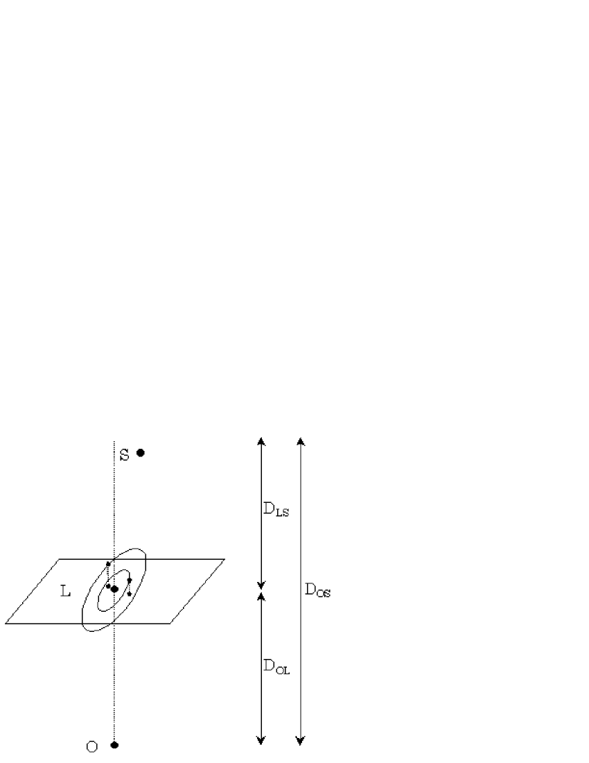
Figure 1: Tipical scheme of planetary lensing.

2 Planetary lensing

A planetary system is nothing but a discrete set of Schwarzschild lenses in a small portion of the space. Fig. 1 shows the typical situation of planetary lensing. The lens plane is defined as a plane orthogonal to the line of sight situated on the barycentre of the lens mass distribution. According to the ordinary theory of lensing (Schneider, Ehlers & Falco, 1992), if the scale of this distribution is much smaller than the distances separating the lens from the source and the observer, then one can deal with the density projected on the lens plane instead of considering the original volume density. This hypothesis is quite verified in real observations where the typical distances are at least of the order of kpc. This consideration can be important in planetary systems where very far planets can eventually have projections enough near to the central star to give perturbations comparable to those of planets placed in more favourable positions. This means that multiple events could be less out of common than one could think (Wambsganns, 1997; Gaudi, Naber & Sackett, 1998). So, it is desirable to preserve the whole planetary system as much as possible before abandoning it for the simplest case of the single planet around the big star. We shall see that the perturbative theory has the considerable advantage of being rather insensitive to the number of planets as regards the difficulty of the problem.

Let’s define the length $R_{E}^{\odot}=\sqrt{\frac{4GM_{\odot}}{c^{2}}\frac{D_{LS}D_{OL}}{D_{OS}}}$. $\mathbf{x}=\left(x_{1};x_{2}\right)$ shall denote the coordinates in the lens plane normalized to $R_{E}^{\odot}$, while $\mathbf{y}=\left(y_{1};y_{2}\right)$ shall be the coordinates in the source plane normalized to $R_{E}^{\odot}\frac{D_{OS}}{D_{OL}}$. $m_{1}$ will be the mass of the central star and $m_{2}$, …, $m_{n}$ will be the masses of the planets. All of these masses are meant to be measured in solar masses. The star will always be placed at the origin, while the projection on the lens plane of the i_th planet will be denoted by $\mathbf{x}_{i}=\left(x_{i1};x_{i2}\right)$. With these notations, the lens equation reads:

$$\mathbf{y}=\mathbf{x}-\frac{m_{1}\mathbf{x}}{\left|\mathbf{x}\right|^{2}}-\sum\limits_{i=2}^{n}\frac{m_{i}\left(\mathbf{x}-\mathbf{x}_{i}\right)}{\left|\mathbf{x}-\mathbf{x}_{i}\right|^{2}}$$ (1)

In (1), the deviation of light rays due to the star has been explicitly separated by those of the planets. Given a source position $\mathbf{y}$, the corresponding $\mathbf{x}$ solving the lens equation are called images.

Many interesting properties of this vectorial application can be studied through its Jacobian matrix. In particular, the determinant of this matrix contains nearly all the information about the properties of the images. Let’s write the Jacobian determinant for the case of planetary lensing using (1):

$$\det J=1-\left[\frac{m_{1}\left(x_{1}^{2}-x_{2}^{2}\right)}{\left(x_{1}^{2}+x_{2}^{2}\right)^{2}}+\sum\limits_{i=2}^{n}\frac{m_{i}\left(\Delta_{i1}^{2}-\Delta_{i2}^{2}\right)}{\left(\Delta_{i1}^{2}+\Delta_{i2}^{2}\right)^{2}}\right]^{2}+\\ -4\left[\frac{m_{1}x_{1}x_{2}}{\left(x_{1}^{2}+x_{2}^{2}\right)^{2}}+\sum\limits_{i=2}^{n}\frac{m_{i}\Delta_{i1}\Delta_{i2}}{\left(\Delta_{i1}^{2}+\Delta_{i2}^{2}\right)^{2}}\right]^{2}$$ (2)

where $\mathbf{\Delta}_{i}=\left(\Delta_{i1};\Delta_{i2}\right)=\mathbf{x}-\mathbf{x}_{i}.$ Given an image I at position $\mathbf{x}_{I}$, the sign of $\det J\left(\mathbf{x}_{I}\right)$ is called the parity of I. It can be proved that the amplification of the image I is given by

$$\mu_{I}=\frac{1}{\left|\det J\left(\mathbf{x}_{I}\right)\right|}$$ (3)

We see from this equation that when $\det J$ is null, the amplification diverges. This is rigorously true for point sources (in ray optics), while for finite (real) sources the integration over the source’s surface makes the amplification finite (Witt & Mao, 1994). The points where $\det J$ vanishes are called critical points, the corresponding points in the source plane through (1) constitute the caustics. So, a point source crossing a caustic will produce images with infinite amplification. Real sources crossing caustics by some of their parts will be highly (but not infinitely) amplified.

The structure of critical curves and caustics provides a substantial description of the general behaviour of the lens (number and roughly location of the images can be established). In microlensing, it is possible to give a qualitative description of light curves just checking whether the track of the source threads some caustic or not.

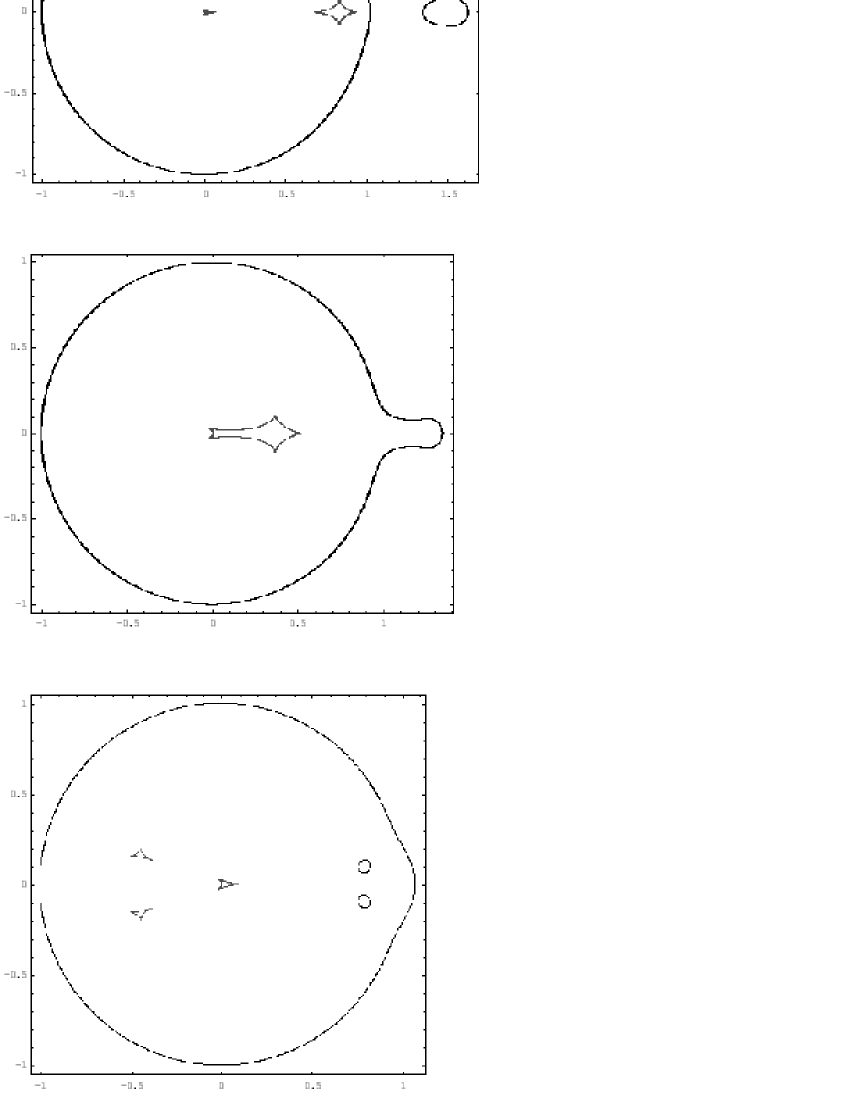
Figure 2: There are three possible situations in planetary lensing as regards critical curves, shown in these plots. The smooth round curves are critical curves, while the small cusped curves are the corresponding caustics.

In fig. 2 the (numerically obtained) critical curves and the caustics of a star with a single planet are shown. There are three possible cases in such a situation. I recall that for a single point source the critical curve is a ring with radius given by its Einstein radius $\sqrt{m}$, while the caustic is a point in the origin of the source plane. When the planet is far beyond the star’s Einstein ring, there is only a small perturbation of the two rings which lends finite extension to the originally point - like caustics. This is much more evident in the planetary caustic which is also displaced towards the star. When the planet is in the proximity of the star’s Einstein ring, the two critical curves merge and so do the caustics. In the last situation where the planet is internal to the star’s Einstein ring, the star’s critical curve returns to be very near to a ring while the planet’s critical curve turns into two ovals to which a couple of triangular caustics correspond behind the star.

3 Caustics and perturbative analysis

In the solar system, the mass ratios between planets and the sun are always less than one thousandth. Jupiter is $9.4\times 10^{-4}M_{\odot}$. Other planets are even less: Earth is $3\times 10^{-6}M_{\odot}$. With these numbers, it is natural to expect that the presence of planets should cause only little perturbations to the single lens case. Upon this consideration the perturbative hypothesis is based. In this and the following section the ratios between planetary and stellar masses will play the role of perturbative expansions parameters. We shall see that in most cases a first order expansion is sufficient to get very reliable results.

Let’s turn to the caustics of planetary systems. First I shall examine the modifications induced in the star’s Einstein ring and consequently the central caustic. Then I shall deal with planetary caustics.

3.1 Central caustic

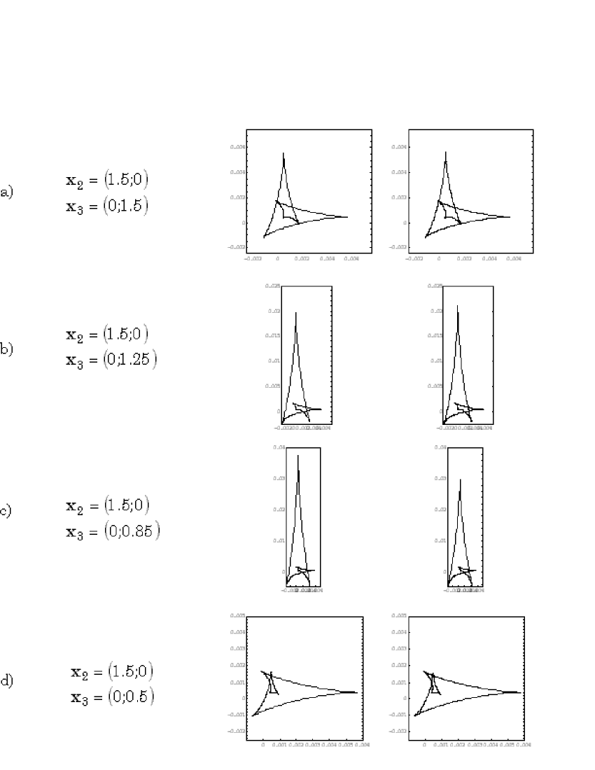
Figure 3: Central caustic for Jovian planets. The caustics on the left are those found perturbatively, while those on the right are obtained numerically. Little differences occur when one of the planets is close to the star’s Einstein ring.

Of course, the starting point for the study of critical curves is the equation $\det J=0$, which can easily be written in polar coordinates:

$$\left[\frac{m_{1}\left(\cos^{2}\vartheta-\sin^{2}\vartheta\right)}{r^{2}}+\sum\limits_{i=2}^{n}\frac{m_{i}\left(\Delta_{i1}^{2}-\Delta_{i2}^{2}\right)}{\left(\Delta_{i1}^{2}+\Delta_{i2}^{2}\right)^{2}}\right]^{2}+\\ +4\left[\frac{m_{1}\sin\vartheta\cos\vartheta}{r^{2}}+\sum\limits_{i=2}^{n}\frac{m_{i}\Delta_{i1}\Delta_{i2}}{\left(\Delta_{i1}^{2}+\Delta_{i2}^{2}\right)^{2}}\right]^{2}=1$$ (4)

Here $\mathbf{\Delta}_{i}=\left(r\cos\vartheta-x_{i1};r\sin\vartheta-x_{i2}\right)$. Expanding this equation to the first order in $m_{i}$, we get:

$$\frac{m_{1}^{2}}{r^{4}}+\frac{2m_{1}\left(\cos^{2}\vartheta-\sin^{2}\vartheta\right)}{r^{2}}\sum\limits_{i=2}^{n}\frac{m_{i}\left(\Delta_{i1}^{2}-\Delta_{i2}^{2}\right)}{\left(\Delta_{i1}^{2}+\Delta_{i2}^{2}\right)^{2}}+\\ +\frac{8m_{1}\sin\vartheta\cos\vartheta}{r^{2}}\sum\limits_{i=2}^{n}\frac{m_{i}\Delta_{i1}\Delta_{i2}}{\left(\Delta_{i1}^{2}+\Delta_{i2}^{2}\right)^{2}}=1$$ (5)

The zeroth order solution is simply $r=\sqrt{m_{1}}$, i.e. the Einstein ring. Let’s write the first order solution as:

$$r=\sqrt{m_{1}}\left(1+\varepsilon\left(\vartheta\right)\right)$$ (6)

with $\varepsilon\ll 1$. Substituting in (5) and expanding to the first order in $\varepsilon$. The zeroth order solution cancels and $\varepsilon$ is found solving the remaining first degree equation:

$$\varepsilon\left(\vartheta\right)=\frac{1}{2}\left(\cos^{2}\vartheta-\sin^{2}\vartheta\right)\sum\limits_{i=2}^{n}\frac{m_{i}\left[\left(\Delta_{i1}^{0}\right)^{2}-\left(\Delta_{i2}^{0}\right)^{2}\right]}{\left[\left(\Delta_{i1}^{0}\right)^{2}+\left(\Delta_{i2}^{0}\right)^{2}\right]^{2}}+\\ +2\sin\vartheta\cos\vartheta\sum\limits_{i=2}^{n}\frac{m_{i}\Delta_{i1}^{0}\Delta_{i2}^{0}}{\left[\left(\Delta_{i1}^{0}\right)^{2}+\left(\Delta_{i2}^{0}\right)^{2}\right]^{2}}$$ (7)

where $\mathbf{\Delta}_{i}^{0}=\left(\sqrt{m_{1}}\cos\vartheta-x_{i1};\sqrt{m_{1}}\sin\vartheta-x_{i2}\right)$ is $\mathbf{\Delta}_{i}$ to the zeroth order.

By very few steps we have found the perturbation of the Einstein ring in a very simple way. The parametric equation of the central caustic is soon found by applying the lens equation (1) and expanding again to the first order in $m_{i}$:

$$y_{1}\left(\vartheta\right) =2\sqrt{m_{1}}\varepsilon\left(\vartheta\right)\cos\vartheta-\sum\limits_{i=2}^{n}\frac{m_{i}\Delta_{i1}^{0}}{\left[\left(\Delta_{i1}^{0}\right)^{2}+\left(\Delta_{i2}^{0}\right)^{2}\right]}$$ (8a)

$$y_{2}\left(\vartheta\right) =2\sqrt{m_{1}}\varepsilon\left(\vartheta\right)\sin\vartheta-\sum\limits_{i=2}^{n}\frac{m_{i}\Delta_{i2}^{0}}{\left[\left(\Delta_{i1}^{0}\right)^{2}+\left(\Delta_{i2}^{0}\right)^{2}\right]}$$ (8b)

Of course, perturbative results are characterized by precise limits of validity. In our case we see that when the denominators in (7) vanish the perturbation diverges. This is not allowed by our assumption that $\varepsilon$ must be very small with respect to the unity. Those denominators represent the distance between the planet and the general point of the unperturbed star’s Einstein ring. So we expect the perturbative theory to fail in those portions of the critical curve which are very near to one of the planets at least. We can understand this “failure” if we look back at fig. 2b: when the planet is close to the star’s Einstein ring, there is only one critical curve which is somewhat different from the ring in the proximity of the planet. For some values of $\vartheta$, the radial coordinate describing the critical curve assumes also more than one value; this situation cannot be described by a first order approximation, where, as we saw, the perturbation solves a first degree equation.

The most interesting aspect of eqs. (7) and (3) is that they are comprehensive of the action of the whole planetary system: they are valid for an arbitrary number of planets, not only the classically investigated case of the single planet. So these formulas enjoy a very high generality and can be used in more realistic contexts. We also note that the contributions coming from different planets superpose without interfering. This is an obvious consequence of the first order approximation; if I had included second order terms, I would have found “interaction” between planets. These “interaction” terms are thus not relevant in a first approximation.

Now let’s compare the perturbative caustics with those found by classical numerical algorithms to test the validity of the perturbative approach. In fig. 3 I show the results for the case of two Jovian planets placed in several positions. When the planets are far enough from the Einstein ring (fig. 3a, 3d), the caustic found according to (3) is entirely identical to the numerical one. Letting one of the planets approach the Einstein ring, a small deviation begins appearing in the region coming from the portion of the Einstein ring that is closest to the planet. This deviation manifests itself in the size of the largest cusp. For Jovian planets these discrepancies unveil at distances from the star’s Einstein ring of the order of a tenth of the Einstein radius. These first encouraging results become much better in the case of Earth - like planets. We expect the range of validity of perturbative results to be increased for this kind of planets, because of their smaller mass. Fig. 4 shows that for these little planets things go very well down to a hundredth of the Einstein radius.

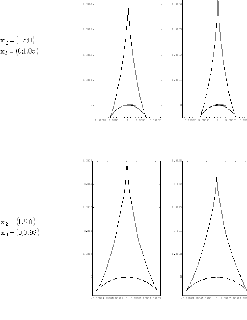
Figure 4: Central caustics for Earth - like planets. The perturbative ones are on the left and the numerical on the right.

So the perturbative method is likely to provide reliable results at the first order already. Moreover, it is not to be forgotten that, in principle, the approximations can be improved pushing farther the perturbative expansion.

3.2 Planetary caustics

Planetary caustics are usually studied considering the planet as a point-lens with an external shear due to the star’s gravitational field (Schneider, Ehlers & Falco, 1992). This kind of lens was introduced by Chang & Refsdal (1979; 1984) in a cosmological context. However, this lens is valid in planetary systems only to the lowest non-trivial order in $m_{i}$. Therefore a correct study should only retain the lowest order terms in the critical curves equation, so that Chang & Refsdal’s caustics are a suitable approximation at the lowest order only and not beyond.

In order to complete the discussion of caustics in planetary systems and study their features properly, in this subsection I derive planetary caustics from perturbative hypothesis paying full attention to the order of each term. The situation for planetary caustics is rather different from that of the central caustic. There is no zeroth order solution to start from, since their very presence is perturbative. Nevertheless this is not a great problem: in fact we shall just search for the lowest order solution of the critical curves equation.

To achieve this, I now rewrite $\det J=0$ in polar coordinates choosing the planet $m_{2}$ situated in $\mathbf{x}_{2}$ as the origin:

$$\left[\frac{m_{1}\left(\Delta_{11}^{2}-\Delta_{12}^{2}\right)}{\left(\Delta_{11}^{2}+\Delta_{12}^{2}\right)^{2}}+\frac{m_{2}\left(\cos^{2}\vartheta-\sin^{2}\vartheta\right)}{r^{2}}+\right.\\ \left.+\sum\limits_{i=3}^{n}\frac{m_{i}\left(\Delta_{i1}^{2}-\Delta_{i2}^{2}\right)}{\left(\Delta_{i1}^{2}+\Delta_{i2}^{2}\right)^{2}}\right]^{2}+4\left[\frac{m_{1}\Delta_{11}\Delta_{12}}{\left(\Delta_{11}^{2}+\Delta_{12}^{2}\right)^{2}}+\right.\\ \left.+\frac{m_{2}\sin\vartheta\cos\vartheta}{r^{2}}+\sum\limits_{i=3}^{n}\frac{m_{i}\Delta_{i1}\Delta_{i2}}{\left(\Delta_{i1}^{2}+\Delta_{i2}^{2}\right)^{2}}\right]^{2}=1$$ (9)

When the planet is very far from the star, we know that its critical curve tends to an Einstein ring with radius $r=\sqrt{m_{2}}$. So we search for critical curves solving (9) with $r\sim\sqrt{m_{2}}$. Let’s save the lowest order terms only. In this operation, the contributions coming from the other planets are ejected out from the equation. It is convenient to place the star in the usual position $(-x_{p};0)$. What remains is:

$$\frac{m_{1}^{2}}{x_{p}^{4}}+\frac{m_{2}^{2}}{r^{4}}+\frac{2m_{1}m_{2}}{x_{p}^{2}r^{2}}\left(\cos^{2}\vartheta-\sin^{2}\vartheta\right)=1$$ (10)

which is biquadratic in $r$. The solution is:

$$r=\sqrt{m_{2}\frac{\frac{m_{1}}{x_{p}^{2}}\cos 2\vartheta\pm\sqrt{1-\frac{m_{1}^{2}}{x_{p}^{4}}\sin^{2}2\vartheta}}{\left(1-\frac{m_{1}^{2}}{x_{p}^{4}}\right)}}$$ (11)

which verifies our assumption $r\sim\sqrt{m_{2}}$. The parametric equations of caustics can be found in the usual way substituting (11) in the lens application and expanding to the first non trivial order ($\sqrt{m_{2}}$):

$$y_{1} = x_{p}-\frac{m_{1}}{x_{p}}\left(1-\frac{r}{x_{p}}\cos\vartheta\right)+\left(r-\frac{m_{2}}{r}\right)\cos\vartheta$$ (12a)

$$y_{2} = -\frac{m_{1}}{x_{p}^{2}}r\sin\vartheta+\left(r-\frac{m_{2}}{r}\right)\sin\vartheta$$ (12b)

The contributions from the other planets are again of higher order. So the structure of planetary caustics is not affected by the presence of other planets at the lowest order in a perturbative expansion. These formulas can thus be used in a single planet situation as well as in a rich planetary system.

Observe that $r$ goes to infinity as $x_{p}$ tends to $\sqrt{m_{1}}$, i.e. when the planet is next to the star’s Einstein radius. So the perturbative results will not be valid in this situation. The reason is the same discussed for the central caustic. The merging of the two caustic is not describable in the lowest order perturbative expansion. Moreover, there’s another limit to be taken in account. I have eliminated all the terms coming from the other planets because of their higher order. But these terms can become dominant when their denominators are small. This happens when one of these planets is close to the planet we are examining. This is not an exotic situation since we must always remember that what counts is actually the projection of the positions on the lens plane. So planets could be very far apart but have near projections yielding exotic critical curves.

We see that the critical curves traced by (11) have two branches according to the double sign in their expression. For planets external to the star’s Einstein ring ( $x_{p}>\sqrt{m_{1}}$), the branch coming from the positive sign is real while the other coming from the negative sign is imaginary for all values of $\vartheta$, being $\left|\frac{m_{1}}{x_{p}^{2}}\cos 2\vartheta\right|<\sqrt{1-\frac{m_{1}^{2}}{x_{p}^{4}}\sin^{2}2\vartheta}$. For internal planets ( $x_{p}<\sqrt{m_{1}}$), the denominator is negative and $\left|\frac{m_{1}}{x_{p}^{2}}\cos 2\vartheta\right|>\sqrt{1-\frac{m_{1}^{2}}{x_{p}^{4}}\sin^{2}2\vartheta}$. So the two branches are both real for:

$$\sin^{2}2\vartheta<\frac{x_{p}^{4}}{m_{1}^{2}};\text{ \ }\cos 2\vartheta<0$$ (13)

that is in two small regions around $\vartheta=\frac{\pi}{2}$ and $\vartheta=\frac{3\pi}{2}$. They are both imaginary elsewhere. All these results are coherent with the behaviour exposed in fig. 2. We have one planetary caustic for external planets and two disconnected caustics for internal planets.

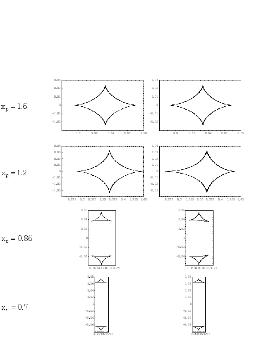
Figure 5: Planetary caustics for a Jovian planet. The caustics on the left column are perturbative while the ones on the right are numerical.

Fig. 5 shows the comparison with the numerical caustics. In fig. 5b the discrepancy with the numerical results appears as a loss of symmetry of the numerical caustic which is elongated towards the central star. This effect is not present in the perturbative Chang & Refsdal’s one. For internal planets near the star’s Einstein ring, the basis of the triangular perturbative caustic is parallel to the star - planet axis(fig. 5c). So Chang & Refsdal’s lens works good until the field can be taken as uniform. When the spherical symmetry becomes important, the caustics begin to differ from perturbative ones. These effects can be taken into account by considering higher order terms in the expansion. These terms would provide the right corrections to the Chang & Refsdal’s approximation.

Eqs. (11) and (11) can be employed to find interesting characteristics of planetary caustics. For example, let’s find the position of the couple of caustics for internal planets. We saw that the critical curves are centered upon $\vartheta=\frac{\pi}{2}$ and $\vartheta=\frac{3\pi}{2}$. Consider the first of these (the other is similar at all). Inserting these values of $\vartheta$ in (11), the possible values of $r$ are:

$$r=\sqrt{m_{2}\frac{-\frac{m_{1}}{x_{p}^{2}}\pm 1}{\left(1-\frac{m_{1}^{2}}{x_{p}^{4}}\right)}}$$ (14)

The point

$$r=x_{p}\sqrt{\frac{m_{1}m_{2}}{m_{1}^{2}-x_{p}^{4}}}$$ (15)

obtainable by a quadratic mean from the two values, is internal to the critical curve and gives an approximation for its position. Immediately, using the lens equation and expanding to the lowest order terms, we find the position of the caustics:

$$y_{1} = x_{p}-\frac{m_{1}}{x_{p}}$$ (16a)

$$y_{2} = x_{p}\sqrt{\frac{m_{1}m_{2}}{m_{1}^{2}-x_{p}^{4}}}\left[1-\frac{m_{1}}{x_{p}^{2}}-\frac{m_{1}^{2}-x_{p}^{4}}{m_{1}x_{p}^{2}}\right]$$ (16b)

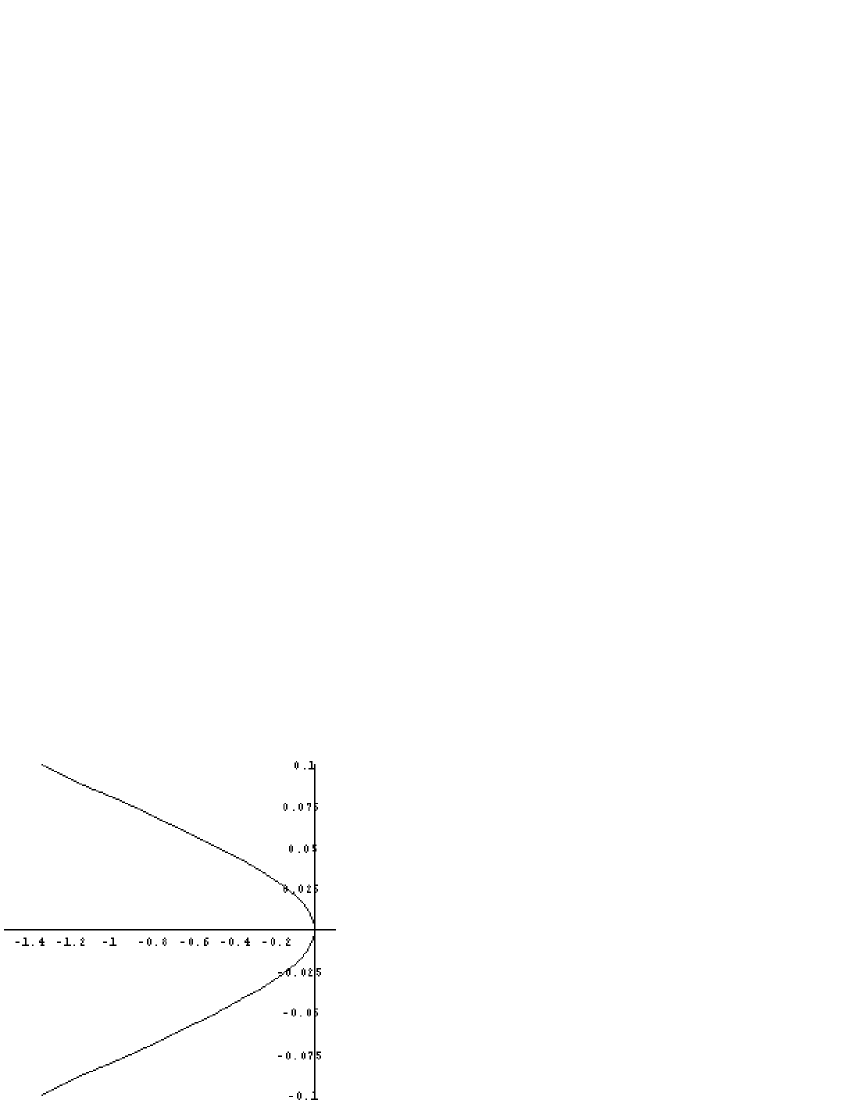
Figure 6: For planets internal to the star’s Einstein ring, the planetary caustics move on this curve.

The first of these is a well known formula (Griest & Safizadeh, 1997). The second completes the information given from the first and allows a complete individuation of the two caustics. Fig. 6 is a plot of the position of the two caustics as a function of the distance of the planet from the star. When $x_{p}\rightarrow 0$ the caustics approximately move on the lines:

$$y_{2}=\pm 2\sqrt{\frac{m_{2}}{m_{1}}}y_{1}$$ (17)

The two planetary caustics delimitate a region of high de - amplification which can appear in microlensing light curves as negative peaks. The positions of the caustics can give a measure of the size of this region and consequently the size of these negative peaks.

3.3 Cusps

This subsection concludes the study of the perturbative caustics with the analysis of the position of cusps in these caustics. The position of cusps can be important in several studies such as microlensing itself. In fact cusps are surrounded by a region with an amplification even higher than that of fold singularities. They also define the extension and the shape of the caustic.

Cusps are defined as the points where the tangent vector of the caustic vanishes. In order to find them we must set

$$\left\{\begin{array}[]{c}y_{1}^{\prime}\left(\vartheta\right)=0\\ y_{2}^{\prime}\left(\vartheta\right)=0\end{array}\right.$$ (18)

and resolve this system of equations for $\vartheta$.

Let’s start with the central caustic. Eqs. (18) after several steps become:

$$\left\{\begin{array}[]{c}\cos\vartheta\left(\frac{\partial\varepsilon}{\partial\vartheta}-\sum\limits_{i=2}^{n}m_{i}\frac{\left(\Delta_{i2}^{0}\cos\vartheta-\Delta_{i1}^{0}\sin\vartheta\right)\left(\Delta_{i1}^{0}\cos\vartheta+\Delta_{i2}^{0}\sin\vartheta\right)}{\left[\left(\Delta_{i1}^{0}\right)^{2}+\left(\Delta_{i2}^{0}\right)^{2}\right]^{2}}\right)=0\\ \sin\vartheta\left(\frac{\partial\varepsilon}{\partial\vartheta}-\sum\limits_{i=2}^{n}m_{i}\frac{\left(\Delta_{i2}^{0}\cos\vartheta-\Delta_{i1}^{0}\sin\vartheta\right)\left(\Delta_{i1}^{0}\cos\vartheta+\Delta_{i2}^{0}\sin\vartheta\right)}{\left[\left(\Delta_{i1}^{0}\right)^{2}+\left(\Delta_{i2}^{0}\right)^{2}\right]^{2}}\right)=0\end{array}\right.$$ (19)

These can simultaneously vanish only if

$$\frac{\partial\varepsilon}{\partial\vartheta}-\sum\limits_{i=2}^{n}m_{i}\frac{\left(\Delta_{i2}^{0}\cos\vartheta-\Delta_{i1}^{0}\sin\vartheta\right)\left(\Delta_{i1}^{0}\cos\vartheta+\Delta_{i2}^{0}\sin\vartheta\right)}{\left[\left(\Delta_{i1}^{0}\right)^{2}+\left(\Delta_{i2}^{0}\right)^{2}\right]^{2}}=0$$ (20)

Explicitly, this equation is:

$$\sum\limits_{i=2}^{n}\frac{m_{i}}{\left[\left(\Delta_{i1}^{0}\right)^{2}+\left(\Delta_{i2}^{0}\right)^{2}\right]^{3}}\left\{3\left[\left(\Delta_{i2}^{0}\right)^{4}-\left(\Delta_{i1}^{0}\right)^{4}\right]\sin\vartheta\cos\vartheta+\right.\\ +3\Delta_{i1}^{0}\Delta_{i2}^{0}\left[\left(\Delta_{i1}^{0}\right)^{2}+\left(\Delta_{i2}^{0}\right)^{2}\right]\left(\cos^{2}\vartheta-\sin^{2}\vartheta\right)+\\ -\Delta_{i1}^{0}\sqrt{m_{1}}\left[\left(\Delta_{i1}^{0}\right)^{2}-3\left(\Delta_{i2}^{0}\right)^{2}\right]\left(4\sin^{3}\vartheta-3\sin\vartheta\right)+\\ \left.+\Delta_{i2}^{0}\sqrt{m_{1}}\left[\left(\Delta_{i2}^{0}\right)^{2}-3\left(\Delta_{i1}^{0}\right)^{2}\right]\left(4\cos^{3}\vartheta-3\cos\vartheta\right)\right\}$$ (21)

which, in despite of its cumbersome aspect, can be exactly solved in the case of the single planet where it yields the four solutions:

$$\vartheta=0\text{; \ }\vartheta=\pi\text{; \ }\\ \vartheta=\pm\arccos\left[\frac{3m_{1}+3x_{p}^{2}-\sqrt{9m_{1}^{2}-14m_{1}x_{p}^{2}+9x_{p}^{4}}}{4\sqrt{m_{1}}x_{p}}\right]$$ (22)

For planetary caustics, we can proceed in a similar way. Multiplying (18a) by $\sin\vartheta$, (18b) by $\cos\vartheta$ and subtracting, we have:

$$\frac{m_{1}}{x_{p}^{2}}r\left(\cos^{2}\vartheta-\sin^{2}\vartheta\right)+2\frac{m_{1}}{x_{p}^{2}}\frac{\partial r}{\partial\vartheta}\sin\vartheta\cos\vartheta-r+\frac{m_{2}}{r}=0$$ (23)

Multiplying by $r$, we get an equation in $r^{2}$ which is easier to handle:

$$\frac{m_{1}}{x_{p}^{2}}r^{2}\left(\cos^{2}\vartheta-\sin^{2}\vartheta\right)+\frac{m_{1}}{x_{p}^{2}}\frac{\partial r^{2}}{\partial\vartheta}\sin\vartheta\cos\vartheta-r^{2}+m_{2}=0$$ (24)

Inserting (11) and solving, we have:

$$\vartheta=0\text{; \ }\vartheta=\frac{\pi}{2}\text{; \ }\vartheta=\pi\text{; \ }\vartheta=\frac{3\pi}{2}$$ (25)

on the higher branch, and:

$$\vartheta = \pm\frac{1}{2}\arcsin\left[\frac{\sqrt{3}x_{p}^{2}}{2m_{1}}\right]\text{;}$$ (26a)

$$\vartheta = \pi\pm\frac{1}{2}\arcsin\left[\frac{\sqrt{3}x_{p}^{2}}{2m_{1}}\right]\text{;}$$ (26b)

$$\vartheta = \frac{\pi}{2}\pm\frac{1}{2}\arcsin\left[\frac{\sqrt{3}x_{p}^{2}}{2m_{1}}\right]\text{;}$$ (26c)

$$\vartheta = \frac{3\pi}{2}\pm\frac{1}{2}\arcsin\left[\frac{\sqrt{3}x_{p}^{2}}{2m_{1}}\right]$$ (26d)

on the lower.

For external planets, the higher branch is complete while the lower is absent, so only the four cusps on the higher branch are actually present. For internal planets, the two branches are real only near $\vartheta=\frac{\pi}{2}$ and $\vartheta=\frac{3\pi}{2}$. So the higher branch has the two cusps at $\vartheta=\frac{\pi}{2}$ and $\vartheta=\frac{3\pi}{2}$, while in the lower one the four cusps (26c) and (26d) are real and the others are imaginary. Summing up we have six cusps distributed in such a way as to form two triangular caustics.

4 Microlensing

Among the numerous forms of gravitational lensing, microlensing is surely one of the most relevant since it opens the possibility of probing the galactic structure through a directly gravitational investigation.

Microlensing occurs when the images of a given source, produced by a small lens, are too close (typically less than $10^{-3}$ arcsecs) to be separated by our telescopes. As we cannot see but a point image of the source, the only way to notice a lensing effect is through a variation of the total light flux coming from the observed source. For a point lens mass, this variation was found by Paczynski (1986) who first thought of galactic microlensing as a new observable astronomical phenomenon. For a planetary system the anomalies in amplification patterns do not enjoy a full analytical description. Our aim is to use a perturbative approach to solve this problem and find analytical light curves for stars accompanied by their planets.

4.1 Paczynski’s curve

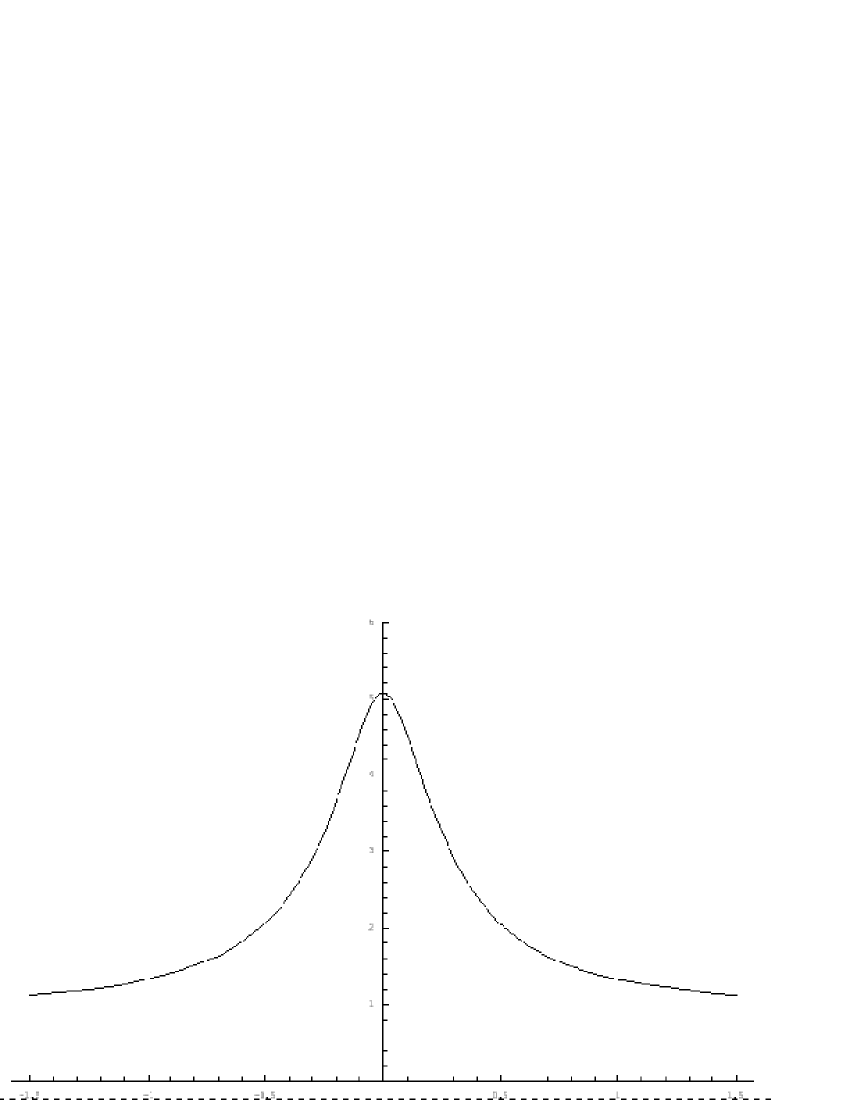
Figure 7: Typical microlensing curve for a point lens mass.

Before considering the problem of planetary microlensing, it is useful to review the steps to be followed in order to get amplification light curves in the event of a single mass (Schneider, Ehlers & Falco, 1992). This will help us in fixing the problems to be faced. In this case, the lens equation takes a very simple aspect:

$$\mathbf{y}=\mathbf{x}-\frac{m_{1}}{\left|\mathbf{x}\right|^{2}}\mathbf{x}$$ (27)

The total amplification is found by summing the amplification of all images. So the first step is to find these images, i.e. the lens equation is to be inverted. Here the task is quite easy, because (27) reduces to a second degree equation whose solutions are:

$$\mathbf{I}^{+} = \frac{\mathbf{y}}{2}\left(1+\frac{\sqrt{4m_{1}+\left|\mathbf{y}\right|^{2}}}{\left|\mathbf{y}\right|}\right)$$ (28a)

$$\mathbf{I}^{-} = \frac{\mathbf{y}}{2}\left(1-\frac{\sqrt{4m_{1}+\left|\mathbf{y}\right|^{2}}}{\left|\mathbf{y}\right|}\right)$$ (28b)

The next step is to compute the amplifications corresponding to each of these images. According to (3), these are:

$$\mu_{I^{\pm}}=\frac{1}{\left|\det J\left(\mathbf{I}^{\pm}\right)\right|}=\frac{1}{\left|1-\frac{m_{1}^{2}}{\left|\mathbf{I}^{\pm}\right|^{4}}\right|}$$ (29)

It is interesting to study the properties of the two images to discover their physical essence (Blandford & Narayan, 1986). The image $\mathbf{I}^{+}$ has positive parity; in the limit of vanishing lensing effect $\left(\left|\mathbf{y}\right|^{2}\gg m_{1}\right)$ $\mathbf{I}^{+}$ tends to $\mathbf{y}$ and its amplification becomes unitary. Thus $\mathbf{I}^{+}$ reduces to the usual image of the source in the absence of lensing. In what follows I’ll refer to it as the principal image. $\mathbf{I}^{-}$ has negative parity and in the limit of low lensing goes as $m_{1}/\left|\mathbf{y}\right|$, while its amplification is always $\mu_{I^{-}}=\mu_{I^{+}}-1$. I shall call it secondary image as it disappears when the lensing effect is not present. Both images are aligned on the line connecting the source and the lens: the principal image is always external to the Einstein ring, while the secondary one is internal to it.

Now we have to sum up the two amplifications to obtain the so - called amplification map:

$$\mu_{TOT}=\frac{2m_{1}+\left|\mathbf{y}\right|^{2}}{\left|\mathbf{y}\right|\sqrt{4m_{1}+\left|\mathbf{y}\right|^{2}}}$$ (30)

This function tells us the amplification corresponding to any given position of the source relatively to the lensing object. Of course it only depends on the distance because of the symmetry of the lens.

The final step is to make the source move along a rectilinear trajectory to obtain the complete light curves corresponding to the passage of a massive lens near the line of sight of the source (obviously it makes no difference who is moving, what counts is only the relative motion). The distance $\left|\mathbf{y}\right|$ is:

$$\left|\mathbf{y}\right|=\sqrt{b^{2}+v_{\bot}^{2}t^{2}}$$ (31)

where $b$ is the impact parameter (the closest approach distance) and $v_{\bot}$ is the projection of the relative speed in a plane orthogonal to the line of sight.

A typical light curve is shown in fig. 7. The height of the maximum is found by substituting the impact parameter in (30). It becomes infinite as $b$ tends to zero. Real sources have finite extensions implying integration processes smoothing the peak of the curve (Witt & Mao, 1994). This cut - off becomes evident when $\left|\mathbf{y}\right|$ is comparable to the source radius.

4.2 The problem of planetary microlensing

In principle, the procedure for attaining microlensing light curves for multiple lenses is the same just expounded for a single point lens. First we should invert the lens application, second we have to compute the amplification of all the images, then sum up to have the amplification map and finally introduce the motion of the source relatively to the lens system. But if we write the lens equation for a star with just one planet placed in $\mathbf{x}_{p}=\left(x_{p},0\right)$:

$$\mathbf{y}=\mathbf{x}-\frac{m_{1}}{\left|\mathbf{x}\right|^{2}}\mathbf{x}-\frac{m_{2}}{\left|\mathbf{x}-\mathbf{x}_{p}\right|^{2}}\left(\mathbf{x}-\mathbf{x}_{p}\right)$$ (32)

we at once see that the inversion is not possible since one must surrender at a fifth degree equation which doesn’t allow to find the images produced by such a lens.

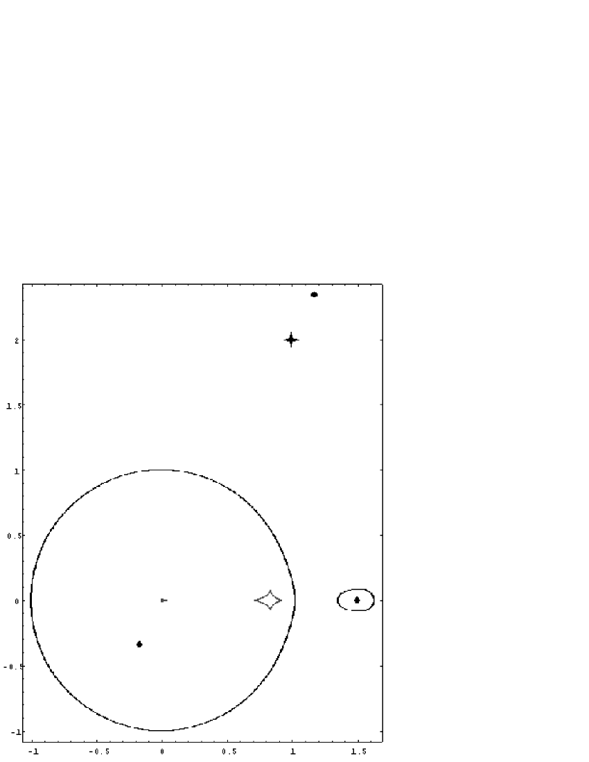
Figure 8: In presence of a planet, a source (here represented by a four-cornered star) placed outside the caustics generates three images (the three little circles in the figure).

A glance at the numerical results can indicate us which way is to be taken in the inversion of the lens application (32). When the source is outside the caustics, only three images are present (see fig. 8). One of them is outside all critical curves and approaches the source when the latter is far enough from the lens. This is indeed the principal image. Another image is inside the star’s critical curve. It is easy to understand that when the mass of the planet vanishes this image becomes the star’s secondary image. The last image is near the planet (inside the planetary critical curve when the planet is external to the star’s Einstein ring). I shall refer to this as the planetary image. It is clear that the presence of the planet slightly perturbs the principal and secondary image of the star, so that their position can be found applying perturbation theory to Paczynski’s images. The planetary image is completely perturbative, since it is not present in the zeroth order situation in which the planet is absent, and must be treated separately. When the source threads a caustic, two new images are formed with opposite parities whose effects are similar to those of the planetary image.

So, the perturbative analysis is likely to be the key to solve the problem of planetary microlensing. In the following two subsections I will use it to discover the images and their amplification. Finally, I will build amplification light curves and compare them with their numerical counterparts.

4.3 Principal and secondary image

Paczynski’s images (7) are the starting point for our expansion and will be generically indicated by the symbol $\mathbf{I}^{\left(0\right)}$. Let’s write the position of the images to the first order in $m_{2}$ as the sum of Paczynski’s image and a small perturbation $\mathbf{\Delta I}$:

$$\mathbf{I}^{\left(1\right)}=\mathbf{I}^{\left(0\right)}+\mathbf{\Delta I}$$ (33)

With this position, in the lens equation expanded to the first order in $m_{2}$

$$y_{1}=I_{1}^{\left(1\right)}-\frac{m_{1}I_{1}^{\left(1\right)}}{\left(I_{1}^{\left(1\right)}\right)^{2}+\left(I_{2}^{\left(1\right)}\right)^{2}}+$$

$$-\frac{m_{2}\left(I_{1}^{\left(0\right)}-x_{p}\right)}{\left(I_{1}^{\left(0\right)}-x_{p}\right)^{2}+\left(I_{2}^{\left(0\right)}\right)^{2}}$$ (34a)

$$y_{2}=I_{2}^{\left(1\right)}-\frac{m_{1}I_{2}^{\left(1\right)}}{\left(I_{1}^{\left(1\right)}\right)^{2}+\left(I_{2}^{\left(1\right)}\right)^{2}}+$$

$$-\frac{m_{2}I_{2}^{\left(0\right)}}{\left(I_{1}^{\left(0\right)}-x_{p}\right)^{2}+\left(I_{2}^{\left(0\right)}\right)^{2}}$$ (34b)

the planetary term no longer contains the perturbation $\mathbf{\Delta I}$. Putting:

$$\Delta y_{1}=\frac{m_{2}\left(I_{1}^{\left(0\right)}-x_{p}\right)}{\left(I_{1}^{\left(0\right)}-x_{p}\right)^{2}+\left(I_{2}^{\left(0\right)}\right)^{2}}\text{;}$$ (35a)

$$\Delta y_{2}=\frac{m_{2}I_{2}^{\left(0\right)}}{\left(I_{1}^{\left(0\right)}-x_{p}\right)^{2}+\left(I_{2}^{\left(0\right)}\right)^{2}}$$ (35b)

and bringing these terms to the left members, we re-gain the structure of the Schwarzschild lens equation (27) in the variable $\mathbf{I}^{\left(1\right)}$ for the source position $\mathbf{y}+\mathbf{\Delta y}$. The planetary induced perturbation can be thus read as a shift in the source position. $\mathbf{I}^{\left(1\right)}$ has the same expression as $\mathbf{I}^{\left(0\right)}$ evaluated in $\mathbf{y}+\mathbf{\Delta y}$ instead of $\mathbf{y}$. The perturbation $\mathbf{\Delta I}$ is found by expanding $\mathbf{I}^{\left(1\right)}$ to the first order in $\mathbf{\Delta y}$:

$$\Delta I_{1}^{\pm}=\frac{\Delta y_{1}}{2}\left(1\pm\frac{\sqrt{4m_{1}+y_{1}^{2}+y_{2}^{2}}}{\sqrt{y_{1}^{2}+y_{2}^{2}}}\right)$$

$$\mp\frac{2m_{1}y_{1}\left(y_{1}\Delta y_{1}+y_{2}\Delta y_{2}\right)}{\sqrt{4m_{1}+y_{1}^{2}+y_{2}^{2}}\sqrt{\left(y_{1}^{2}+y_{2}^{2}\right)^{3}}}$$ (36a)

$$\Delta I_{2}^{\pm}=\frac{\Delta y_{2}}{2}\left(1\pm\frac{\sqrt{4m_{1}+y_{1}^{2}+y_{2}^{2}}}{\sqrt{y_{1}^{2}+y_{2}^{2}}}\right)$$

$$\mp\frac{2m_{1}y_{2}\left(y_{1}\Delta y_{1}+y_{2}\Delta y_{2}\right)}{\sqrt{4m_{1}+y_{1}^{2}+y_{2}^{2}}\sqrt{\left(y_{1}^{2}+y_{2}^{2}\right)^{3}}}$$ (36b)

The upper signs stand for the principal image and the lower for the secondary. The expansion parameter $m_{2}$ appears through $\mathbf{\Delta y}$.

Now the position of the principal and secondary image are known. The most delicate operation is done and the door to the planetary microlensing is open at last. What remains is only mechanic computation without any conceptual difficulties.

The amplification of each image is found by the general formula (3) expanded to the first order in $m_{2}$ (I drop the zero from $\mathbf{I}^{\left(0\right)}$ to simplify notation):

$$\mu_{I}=\frac{1}{\left|1-\frac{m_{1}^{2}}{\left(I_{1}^{2}+I_{2}^{2}\right)^{2}}\right|}\left\{1-\frac{4m_{1}^{2}}{\left(I_{1}^{2}+I_{2}^{2}\right)^{3}}\left(I_{1}\Delta I_{1}+I_{2}\Delta I_{2}\right)+\right.\\ +\frac{2m_{1}m_{2}}{\left(1-\frac{m_{1}^{2}}{\left(I_{1}^{2}+I_{2}^{2}\right)^{2}}\right)}\\ \left.\left[\frac{\left(I_{1}^{2}-I_{2}^{2}\right)\left(\left(I_{1}-x_{p}\right)^{2}-I_{2}^{2}\right)+4I_{1}\left(I_{1}-x_{p}\right)I_{2}^{2}}{\left(I_{1}^{2}+I_{2}^{2}\right)^{2}\left(\left(I_{1}-x_{p}\right)^{2}+I_{2}^{2}\right)^{2}}\right]\right\}$$ (37)

This is the sought formula for the amplification of the images. Paczynski’s amplification multiplies the main brackets containing the sum of all perturbations following the zero order solution represented by the unity. Two kinds of perturbations can be recognized: the first is caused by the previously found shift in the image positions $\mathbf{\Delta I}$; the second is the consequence of the change of the function $\det J$ produced by the presence of the planetary term in the lens equation. I have dropped the modulus from the main brackets because its content is always positive since the perturbations are smaller than unity (except for the zones where perturbative method is no longer valid).

As usual, the validity of perturbation theory is limited to the regions where perturbations are enough small to make sense. So it is necessary a careful examination of the denominators of all perturbative terms. The shift terms present the distance of the zeroth order image from the origin raised to the sixth power. There’s no problem for the principal image which is always far beyond the Einstein ring, but this is not true for the secondary image. However the “failure” rises in the limit of vanishing lensing where the amplification of this image is so low to be totally masked by the amplification of the principal image. When the amplification of the secondary image begins to become important, the distance from the origin is largely sufficient to eliminate all the problems and have fine perturbations. The shift $\mathbf{\Delta I}$ becomes infinite when the source passes through the origin; so the region very near the origin is the first to avoid. The displacement $\mathbf{\Delta y}$ diverges when the zeroth order image approaches the planet as could easily be foreseen for a first order perturbation theory. As regards the terms coming from the alteration of $\det J$, there’s nothing new; the prescriptions are the same as those from the other terms.

In sum we are allowed to use these amplification formulae for all source positions being not too near the origin or generating images too close to the planet. This hardly happens when the source is internal to the caustics. We’ll see that very reliable results can be obtained up to very short distances from the centres of the caustics.

4.4 Planetary image

As previously announced, in this subsection I shall deal with the third image. The presence of this image is absolutely tied to that of the planet. Anyway, Paczynski’s images can still provide a good starting point for our analysis. In fact, if the planet is very far from the star, it too will behave as a single lens. In this case, the planetary image is nothing but the secondary Paczynski’s image for a very low mass. In this limit, its distance from the planet is of order $m_{2}$. So, in our perturbative expansion, we are encouraged to search for images with distances from the planet of order $m_{2}$. Let $\mathbf{I}^{p}$ be the position of the planetary image. We have:

$$\mathbf{I}^{p}=\mathbf{x}_{p}+\mathbf{\Delta I}^{p}$$ (38)

with $\mathbf{\Delta I}^{p}$ of order $m_{2}$. Saving only the lowest order, the lens application reads:

$$y_{1} = x_{p}-\frac{m_{1}}{x_{p}}-\frac{m_{2}\Delta I_{1}^{p}}{\left(\Delta I_{1}^{p}\right)^{2}+\left(\Delta I_{2}^{p}\right)^{2}}$$ (39a)

$$y_{2} = -\frac{m_{2}\Delta I_{2}^{p}}{\left(\Delta I_{1}^{p}\right)^{2}+\left(\Delta I_{2}^{p}\right)^{2}}$$ (39b)

These equations can easily be solved. The solution is:

$$I_{1}^{p} = x_{p}-\frac{m_{2}\left(y_{1}-y_{p}\right)}{\left(y_{1}-y_{p}\right)^{2}+y_{2}^{2}}$$ (40)

$$I_{1}^{p} = -\frac{m_{2}y_{2}}{\left(y_{1}-y_{p}\right)^{2}+y_{2}^{2}}$$ (41)

where $y_{p}=x_{p}-\frac{m_{1}}{x_{p}}$ is the zeroth order position of the planetary caustic already rising in former discussions.

As ever the amplification is calculated by expanding (3). The lowest order result is:

$$\mu_{I^{p}}=\frac{m_{2}^{2}}{\left[\left(y_{1}-y_{p}\right)^{2}+y_{2}^{2}\right]^{2}}$$ (42)

Notice how this formula is much more simple than other images amplification.

The denominators in these expressions vanish when $\mathbf{y}\rightarrow\mathbf{y}_{p}$. Consequently the perturbative method fails when the source is very close to the centre of the planetary caustic.

4.5 Perturbative light curves in planetary microlensing

Once we have found the amplification for each image, in order to obtain the microlensing amplification map we must sum up the components coming from the three images. However, we see that the contribution to the total amplification of the planetary image is of the second order in $m_{2}$. Since we are only considering first order corrections to Paczynski’s curve, this contribution is to be ignored. Therefore, from now on, we shall confine ourselves to the principal and secondary images only.

One consideration is for the two hidden images coming out when the source crosses a caustic. If the event regards the planetary caustic, the two images can be found by carrying further the expansion (38). The new images arise from higher order solutions and their amplifications will also be of higher orders. So we don’t worry about them. On the contrary, if the source crosses the central caustic, the new images appear near the star’s Einstein ring, far from any possible starting point for a perturbative expansion. As we are not taking them into account, we cannot expect to obtain good results inside the central caustic. Anyway, central caustic crossing events are very improbable, since the extension of this caustic is $m_{2}^{2}/m_{1}^{2}$ times the star’s Einstein ring.

Building light curves presents no difficulty. Chosen one source trajectory, it suffices to parameterize $y_{1}$ and $y_{2}$ in the amplification map properly. This is no longer a function of the radial coordinate because there is no more rotational symmetry.

To account for the finite size of the source a simple numerical integration of the perturbative amplification map on the source area at each point of the trajectory can be performed. The curves thus obtained can be compared to numerical ones given by “inverse ray shooting” algorithm.

All the results I show in this paper regard a system constituted by a star with mass $m_{1}=1$ and a Jovian planet ($m_{2}=10^{-3}$). This choice has been made in order to put in better evidence planetary perturbations and to test the perturbative approach in the least favourable situation. Obviously with Earth - like planets things can only go better.

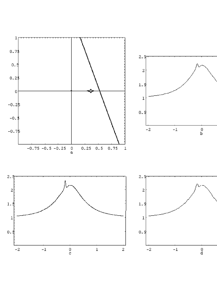
Figure 9: Besides a star with unitary mass placed in the origin, here is a Jovian planet ($m_{2}=10^{-3}$) in $\mathbf{x}_{p}=\left(1.2;0\right)$. The trajectory of the source shown in (a) has impact parameter 0.5. (b) is a numerical light curve obtained by “inverse ray shooting” for a source 43 times greater than the sun. (c) is the perturbative light curve for a point source and (d) is the same curve after a numerical integration over the source extension.

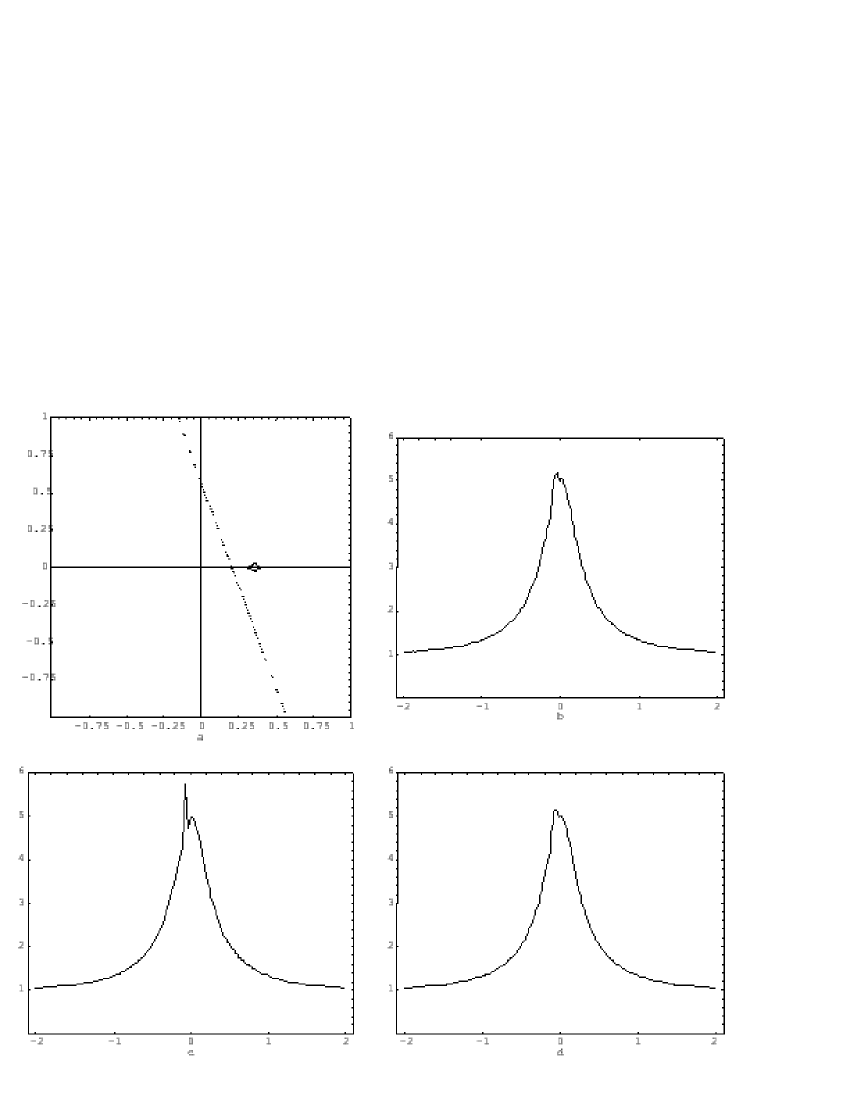
Figure 10: Same lens system and same figure ordering as before. The impact parameter is 0.2.

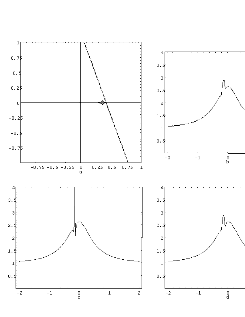
Figure 11: The lens system is the same again but the impact parameter 0.4 makes the source cross the planetary caaustic.

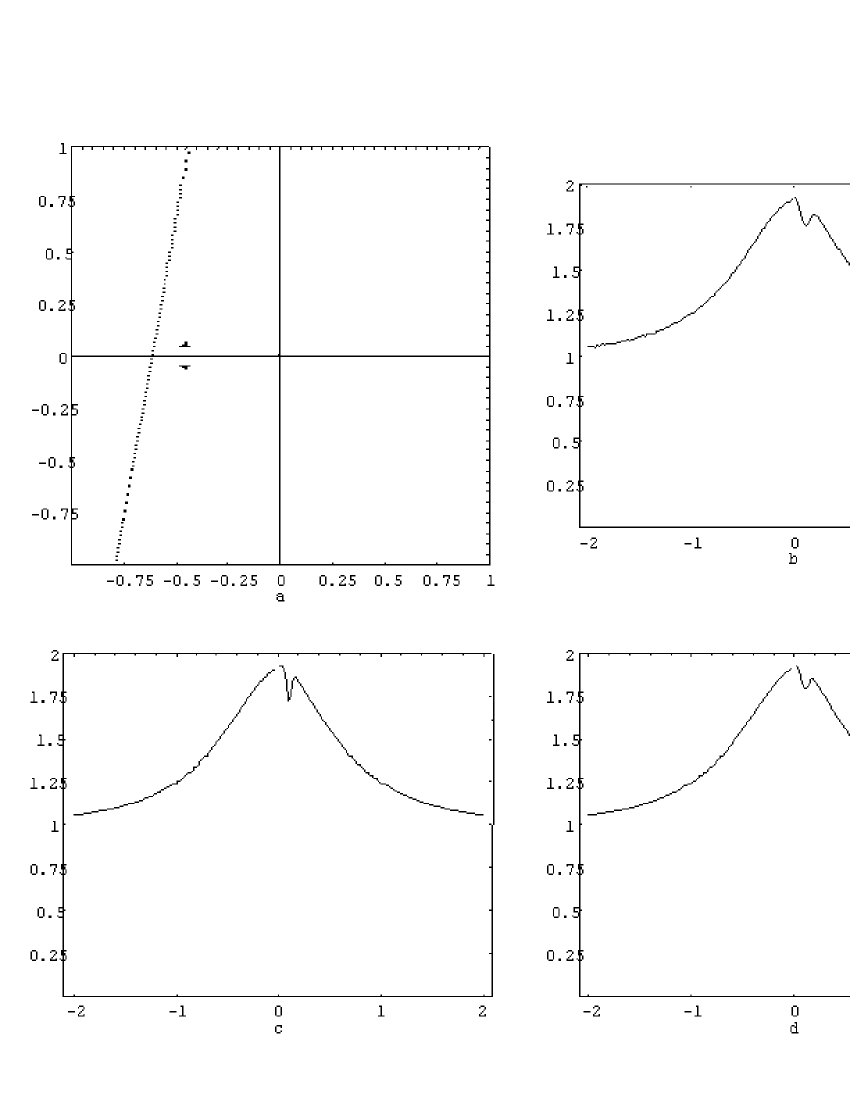
Figure 12: Now the planet is in $\mathbf{x}_{p}=\left(0.8,0\right)$. The three light curves are obtained in the same ways described in fig. 9. The impact parameter is 0.6.

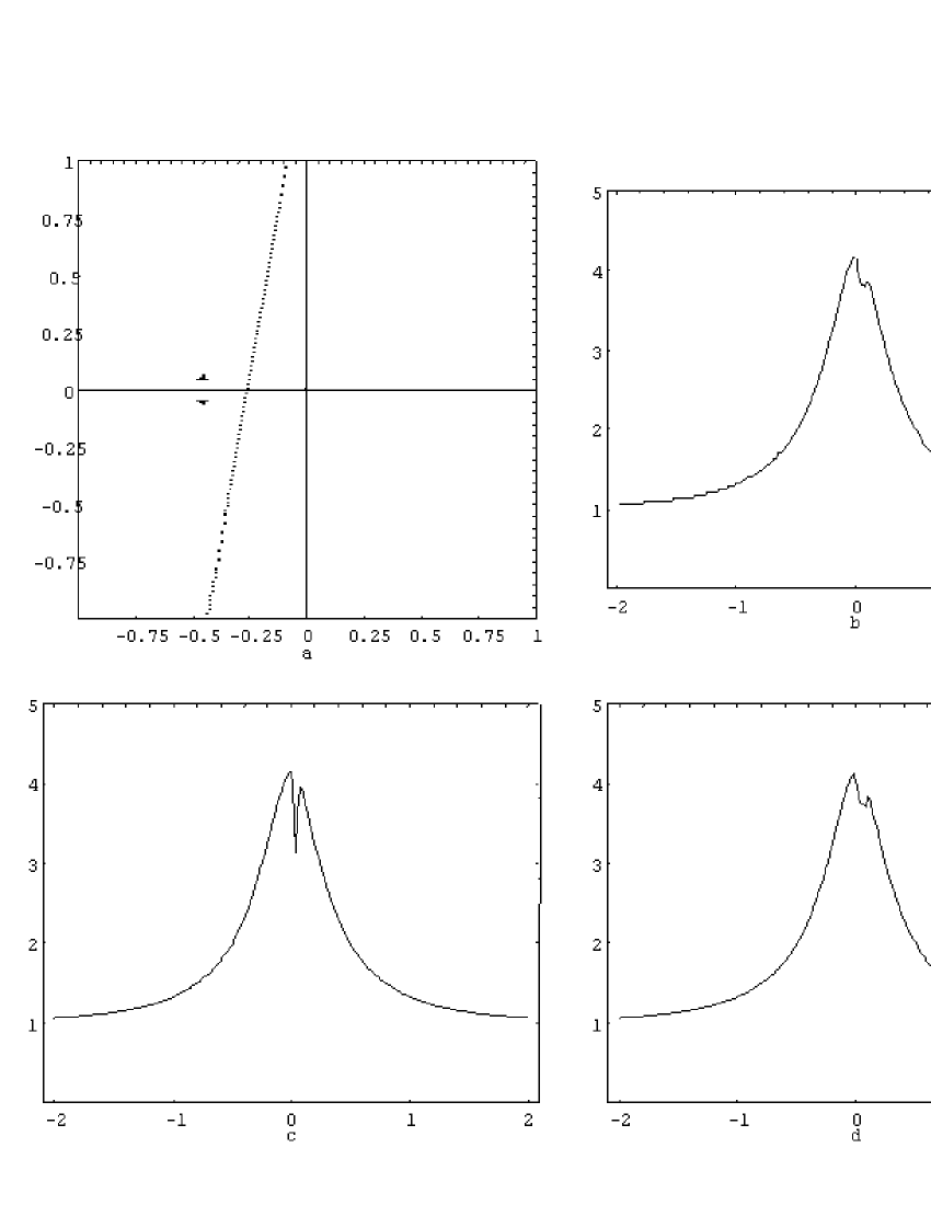
Figure 13: Same lens system as in the previous figure. The impact parameter is 0.25.

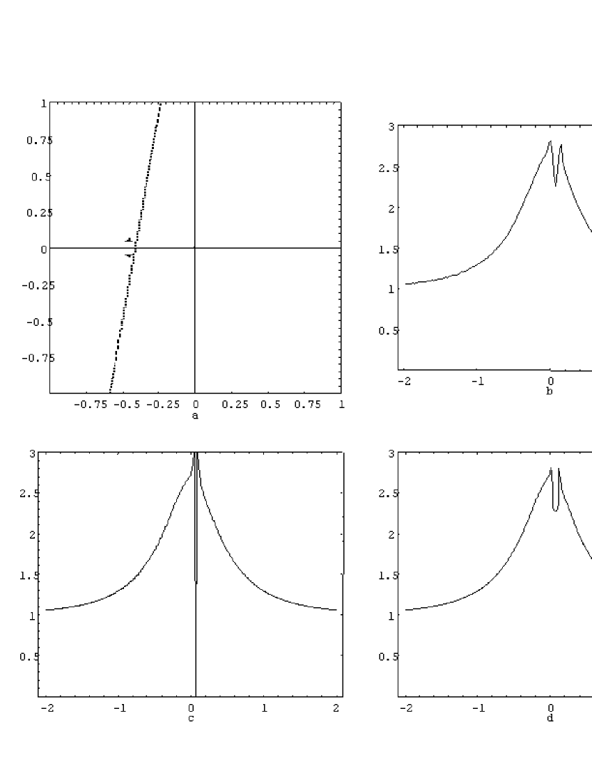
Figure 14: Caustic crossing with impact parameter 0.4.

Let’s start with an external planet. In fig. 9 the planet is in $x_{p}=1.2$. The trajectory chosen for this first test is shown in fig. 9a and has impact parameter 0.5. The numerically attained light curve is displayed in fig. 9b. The source used for this curve has radius 0.045. In a standard observation towards the bulge of the galaxy ($D_{OL}\sim 8kpc$, $D_{OS}\sim 10kpc$), this value would correspond to a giant about 43 times greater than the sun. Here the presence of the planet is responsible for the little peak on the left of the maximum of the curve. Fig. 9c represents the perturbative light curve for a point source moving along the same trajectory. If we perform the numerical integration of the perturbative amplification map, as previously said, the perturbative light curve 9d becomes indistinguishable from the numerical one.

This is a very encouraging result, so let’s choose other trajectories to see other tests. In fig. 10 the position of the planet is the same but the trajectory passes between the planetary caustic and the central caustic at a minimum distance of 0.2. The peak in the numerical curve 10b is very close to the maximum. The point source perturbative curve 10c presents a sharp peak which assumes the right proportions after the integration in 10d.

At this point, let’s see what happens when the source crosses the planetary caustic. In fig. 11a, the impact parameter 0.4 allows the crossing. The peak in the numerical curve 11b becomes considerably high. In the point source perturbative curve 11c the peak is very sharp (it would diverge at the centre of the caustic $\mathbf{y}_{p}$). However, the integration over the source surface still succeeds in reporting this peak to the right size and shape.

Now, let’s consider an internal planet ($x_{p}=0.8$). The region between the couple of planetary caustic is characteristic for its high de-amplification. This produces negative peaks on light curves such as the one shown in fig. 12b corresponding to the trajectory in fig. 12a. It is interesting to see that the perturbative method reproduces this situation with the same great accuracy proved in the former situations. As ever, the point source peak in 12c is smoothed by finite source effect in 12d.

In fig. 13 the impact parameter is 0.25 and things go perfectly as previously.

Finally, let’s consider caustic crossing in this case. Fig. 14a shows a trajectory very close to the planetary caustics. The “inverse ray shooting” curve 14b presents a large de-amplification preceded and followed by little positive peaks. The perturbative curve 14c is characterized by the same situation but the de-amplification is so high to make the total amplification become (unphysically) negative. Now let’s see what happens with a finite source. Because of its extension, part of the source hits the centre of the caustic $\mathbf{y}_{p}$ where the perturbative amplification map diverges. This is a hard problem for the numerical integration which becomes very unstable in this zone, so the bottom of the de-amplification region of the light curve 14d cannot be taken as significant. However, we see that things go fairly well even in this extreme situation.

5 Conclusions

The success of perturbative theory in planetary lensing cannot but impress for the simplicity of the calculations involved and the surprising accuracy of the results even in the hardest situations.

In the derivation of the caustics of a planetary system, by a simple idea and very few passages the complete structure of these curves has been easily obtained. The almost complete insensitivity of the perturbative approach to the number of the planets allows complete descriptions of planetary systems without any loss of generality. Also many important physical assertions can be stated thanks to these results. The fact that the shape of the central caustic is largely given by a linear superposition of the effects of  the single planets is indeed remarkable.

In planetary microlensing the results are even exalting. The perturbative amplification map allows the construction of very fine light curves. In the derivation of the amplification map I have dealt with only one planet for the sake of simplicity. Yet the generalization to an arbitrary number of planets is immediate because in the first order domain a superposition principle is here valid as well. For point sources, light curves can be attained in a completely analytical way, while for finite sources I have resorted to numerical integration until now. Work to englobe finite source effect in the analytical description is in progress. When these curves are available, the extraction of parameters of planetary systems from microlensing light curves will start on more solid analytical bases. Also it could be possible to use the analytical expressions in experimental fits, though the large number of parameters would greatly affect the uncertainties in their determination.

- (1) Alard, C. et al. (1997), A. & A., 321, 424; 326, 1.
- (2) Alcock, C. et al. (1993), Nature, 365, 621.
- (3) Alcock, C. et al. (1995), ApJ, 454, L125.
- (4) Alcock, C. et al. (1998). ApJ, 491, 436.
- (5) Ansari, R. et al. (1997), A. & A., 324, 843.
- (6) Aubourg, E. et al. (1993), Nature, 365, 623.
- (7) Blandford, R. D. & R. Narayan (1986), ApJ, 310, 568
- (8) Bolatto, D.B. & E.E. Falco (1994), ApJ, 436, 112.
- (9) Gaudi, B.S. & A. Gould (1996), ApJ 486, 85.
- (10) Gaudi, B.S., R.M. Naber and P.D. Sackett (1998), astro-ph/9803282.
- (11) Gould, A. (1992), ApJ, 392, 442.
- (12) Gould, A. & A. Loeb (1992), ApJ, 396, 104.
- (13) Griest, K. & N. Safizadeh (1997), ApJ 500, 37.
- (14) Jetzer Ph., M. Strassle and U. Wandeler, Gravitational microlensing by globular clusters (1998) submitted to A & A.
- (15) Mao, S. & B. Paczynski (1991), ApJ, 374, L37.
- (16) Melchior, A. et al. (1999), A. & A., 134, 377.
- (17) Paczynski, B. (1986), ApJ 301, 503; ApJ 304, 1.
- (18) Peale, S.J. (1997), Icarus, 127, 269.
- (19) Sackett, P.D. (1997), astro-ph/9709269.
- (20) Schneider P., J. Ehlers and E.E. Falco, Gravitational lenses Springer-Verlag, Berlin (1992).
- (21) Schneider, P. & A. Weiss (1986), A & A, 164, 237.
- (22) Sutherland, W. (1998), astro-ph/9811185.
- (23) Tomaney, A.B. & A.P.S. Crotts (1996) Astron. J., 112, 2872.
- (24) Udalski, A. et al. (1993), Acta Astron., 43, 289.
- (25) Udalski, A. et al. (1993), ApJ, 436, L103.
- (26) Wambsganss, J. (1997), MNRAS, 284, 172.
- (27) Witt, H.J. & S. Mao (1994), ApJ, 430, 505.
- (28) Witt, H.J. & A.O. Petters (1993), J. Math. Phys., 34, 4093.