Predicting Stellar Angular Sizes

Abstract

Reliable prediction of stellar diameters, particularly angular diameters, is a useful and necessary tool for the increasing number of milliarcsecond resolution studies being carried out in the astronomical community. A new and accurate technique of predicting angular sizes is presented for main sequence stars, giant and supergiant stars, and for more evolved sources such as carbon stars and Mira variables. This technique uses observed $K$ and either $V$ or $B$ broad-band photometry to predict $V=0$ or $B=0$ zero magnitude angular sizes, which are then readily scaled to the apparent angular sizes with the $V$ or $B$ photometry. The spread in the relationship is 2.2% for main sequence stars; for giant and supergiant stars, 11-12%; and for evolved sources, results are at the 20-26% level. Compared to other simple predictions of angular size, such as linear radius-distance methods or black-body estimates, zero magnitude angular size predictions can provide apparent angular sizes with errors that are 2 to 5 times smaller.

1 Introduction

Prediction of stellar angular sizes is a tool that has come to be used with greater frequency with the advent of high resolution astronomical instrumentation. Structure at the tens to hundreds of milliarcsecond (mas) level is now being routinely observed with the Hubble Space Telescope, speckle interferometry, and adaptive optic systems. Single milliarcsecond observations, selectively available for many years with the technique of lunar occultations, are now becoming less specialized as prototype interferometers in the optical and near infrared evolve towards facility class instruments. For all of these telescopes and techniques, it is often desirable to predict angular size of stars, to select either appropriate targets or calibration sources.

Detailed photometric and spectrophotometric predictive methods provide results with high accuracy (1-2% diameters; cf. Blackwell & Lynas-Gray 1998, Cohen et al. 1996). However, diameters from these methods require large amounts of data that is often difficult to obtain, and as such, are available for a limited number of objects. For the general sample of stars, only limited information is available, and spectral typing, photometry, and parallaxes are all less available and less accurate as one examines stars at greater distances. Deriving expected angular sizes is a greater challenge in this case. Fortunately the general availability of $B$ or $V$ band data, and forthcoming release of the data from the 2MASS and DENIS surveys, which have limiting magnitudes of $K>14.3$ and $13.5$, respectively (Beichman et al. 1998, Epchtein 1997), will provide at least broad-band photometry on these more distant sources. Given these databases, of general utility is a method based strictly upon this widely available data. In this paper a method based solely upon $K$ and either $B$ or $V$ broad-band photometry will be presented, and it will be shown that angular sizes for a wide variety of sources can be robustly predicted with merely two-color information. A similar relationship is discussed by Mozurkewich et al. (1991), who present a ‘distance normalized uniform disk angular diameter’ as a function of $R-I$ color, but with a limited number ($N=12$) of objects to calibrate the relationship. Related to these methods is the study of stellar surface brightness as a function of $V-K$ color published by Di Benedetto (1993), which built on the previous work by Barnes & Evans (Barnes & Evans 1976, Barnes et al. 1976, 1978).

2 Sources of Data

The relationship between angular size and color to be presented in §3 is strictly empirical. The angular sizes and photometry utilized to calibrate the method are all available in the literature, and in many cases are also online, and their sources are presented below.

2.1 Available Angular Size Data

As a test of the method, we shall be examining its predictions against known angular diameters. For stars that have evolved off of the main sequence, angular diameters as determined in the near-infrared are preferred, as limb darkening - and the need for models to compensate for it - is less than at shorter wavelengths. There are four primary sources in the literature of near-infrared angular diameters (primarily K band):

Kitt Peak. The lunar occultation papers by Ridgway and his coworkers (Ridgway et al. 1974, Ridgway 1977, Ridgway et al. 1977, 1979, 1980a, 1980b, 1982a, 1982b, 1982c, Schmidtke et al. 1986) established the field of measuring angular sizes of cool stars in the near-infrared. This effort is no longer active.

TIRGO. The lunar occultation papers by Richichi and his coworkers (Richichi et al. 1988, 1991, 1992a, 1992b, 1995, 1998a, 1998b, 1998c, 1999, Di Giacomo et al. 1991) have further developed this particular technique of diameter determinations. The group is continuing to explore the high-resolution data obtainable from lunar occultations. The recent publications from the TIRGO group include data from medium to large aperture telescopes (1.23m - 3.5m), along with concurrent photometry.

IOTA. The K band angular diameters papers from the Infrared-Optical Telescope Array by Dyck and his coworkers (Dyck et al. 1996a, 1996b, 1998, van Belle et al. 1996, 1997, 1999b) provided a body of information on normal giant and supergiant papers, and also on more evolved sources such as carbon stars and Mira variables. Recently, results from this interferometer using the FLUOR instrument have become available (Perrin et al. 1998).

PTI. Although there is only one angular diameter paper currently available from the Palomar Testbed Interferometer (van Belle et al. 1999a), 69 objects are presented in the manuscript from this highly automated instrument.

Altogether, this collection from the literature represents 92 angular diameters for 67 carbon stars and Miras, and 197 angular diameters for 190 giant and supergiant stars. In addition to these near-infrared observations of evolved objects, shorter wavelength observations were used to obtain diameters for main sequence objects – few near infrared observations exist for these smaller sources. These objects were culled from the catalog by Fracassini et al. (1988), limiting the investigation to direct angular size measures found in that catalog: lunar occultations, eclipsing and spectroscopic binaries, and the intensity interferometer observations of Hanbury Brown et al. (1974). Unfortunately, this sample of 50 main sequence objects is much smaller than the evolved star sample, largely reflecting the current resolution limits of roughly 1 mas in both the interferometric and lunar occultation approaches: a one solar radius object at a distance of 10 pc has an angular size of 0.92 mas. Furthermore, many of main sequence stars did not have sufficient photometry to be used in the technique discussed in §3. Fortunately, added to this sample are the well-calibrated measurements for the Sun (Allen 1973).

Shorter wavelength observations of giant and supergiant stars, while available (eg., Hutter et al. 1989, Mozurkewich et al. 1991), were not utilized in this study for two reasons. First, there are complications arising from reconciling angular diameters inferred from short wavelength ($\lambda<1.2\mu$m) observations with the desired Rosseland mean diameters for these cooler stars. Second, the majority of the data collected on these stars, represented in the Mark III interferometer database, remains unpublished. Fortunately, these data are anticipated to be published soon (Mozurkewich 1999) and will be complimented by additional short-wavelength data from the NPOI interferometer (Nordgren 1999).

2.2 Sources of Photometry

The widespread availability of Internet access, coupled with the electronic availability of most (if not all) of the photometric catalogs, has made task of researching archival photometry much more tractable. When photometry was not directly available from the telescope observations, the archival sources utilized in this investigation were as follows:

General Data. One of the more thorough references on stellar objects is SIMBAD (Egret et al. 1991; http://simbad.u-strasbg.fr/ (France) and http://simbad.harvard.edu/ (US Mirror)). In addition to the web-based query forms, one may also obtain information from SIMBAD by telnet and email. It is important to note that SIMBAD is merely a clearing house of information from a wide variety of sources and is not an original source in and of itself; any information that ends up being crucial to the merit of an astrophysical investigation should be checked against its primary source.

Infrared Photometry ($\lambda>1\mu$m). The Catalog of Infrared Observations (CIO), a extensive collection of IR photometry by Gezari et al. (1993) has been updated, although the most recent version is available only online (Gezari, Pitts & Schmitz 1997). The latter catalog can be queried with individual stars or lists of objects at VizieR (Genova et al. 1997; http://vizier.u-strasbg.fr/ (France) and http://adc.gsfc.nasa.gov/viz-bin/VizieR (US Mirror)). As with the SIMBAD data, the CIO is merely a collection of the data in the literature, and examination of the primary sources is advised. Also, as noted in the introduction, the forthcoming release of the 2MASS and DENIS catalogs will greatly augment the collective database of near-infrared photometry (whose home pages are http://www.ipac.caltech.edu/2mass/ and http://www-denis.iap.fr/denis.html, respectively).

Visual Photometry. The General Catalog of Photometric Data (GCPD) provides a large variety of wide- to narrow-band visual photometric catalogs (Mermilliod et al. 1997; http://obswww.unige.ch/gcpd/gcpd.html). For variable stars, the American Association of Variable Star Observers (AAVSO) and its French counterpart, the Association Française des Observateurs d’Etoiles Variables (AFOEV) are both excellent sources of epoch-specific visible light photometry (Percy & Mattei 1993, Gunther 1996; http://www.aavso.org/ and http://cdsweb.u-strasbg.fr/afoev/, respectively).

3 Zero Magnitude Angular Size versus $V-K$, $B-K$ Colors

The large body of angular sizes now available allows for direct predictions of expected angular sizes, bypassing many astrophysical considerations, such as atmospheric structure, distance, spectral type, reddening, and linear size. To compare angular sizes of stars at different distances, one approach is to scale the sizes relative to a zero magnitude of $V=0$:

$$\theta_{V=0}=\theta\times 10^{V/5}.$$ (1)

The angular size thus becomes a measure of apparent surface brightness (a more detailed discussion of related quantities may be found in Di Benedetto 1993.) Conversion between a $V=0$ zero magnitude angular size, $\theta_{V=0}$, and actual angular size, $\theta$, is trivial with a known $V$ magnitude and the equation above. The same approach has been employed for $K=0$ (see Dyck et al. 1996a) and will also be applied in this paper to $B=0$. Given the general prevalence of $V$ band and the inclusion of $B$ band data in the 2MASS catalog, the apparent angular size approach will be developed here for $V-K$ and $B-K$ colors.

3.1 Evolved Sources: Giant and Supergiant Stars

163 normal giant and supergiant stars found in the interferometry and lunar occultation papers were also found to have available $V$ photometry. By examining their near-infrared angular sizes, we can establish a relationship between $V=0$ zero magnitude angular size and $V-K$ color:

$$\theta_{V=0}=10^{0.669\pm 0.052+0.223\pm 0.010\times(V-K)}.$$ (2)

The errors on the 2 parameters in the equation above are $1\sigma$ errors determined from a $\chi^{2}$ minimization; given 2 degrees of freedom in the equation, $\Delta\chi^{2}=2.30$ about the $\chi^{2}$ minimum for this case (Press et al. 1992). Similar error calculations will be given for all other relationships reported in this manuscript. Examining the distribution of the differences between the fit and the measured values, $\Delta\theta_{V=0}$, we find an approximately Gaussian distribution with the rms value of the 163 differences yielding a fractional error of ${(\Delta\theta_{V=0}/\theta_{V=0})_{rms}}=11.7\%$.

Similarly, for $B-K$ color, 136 giant and supergiant stars had available photometry, resulting in the following fit:

$$\theta_{B=0}=10^{0.648\pm 0.072+0.220\pm 0.012\times(B-K)},$$ (3)

with an rms error of 10.8%.

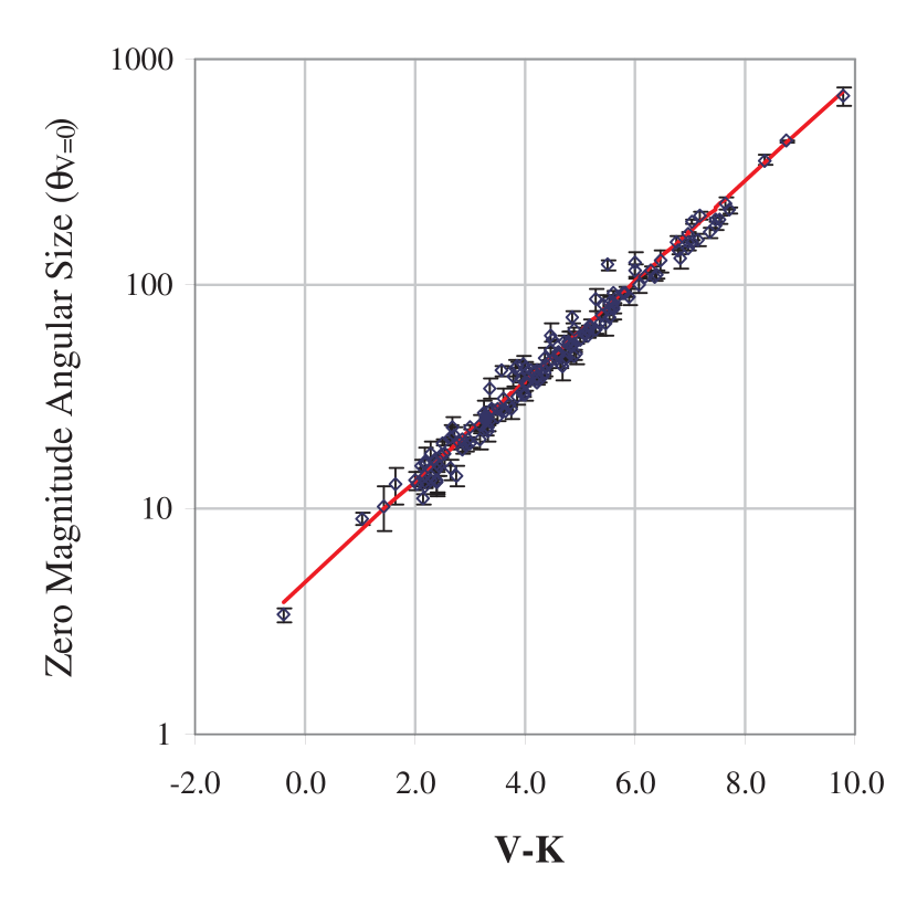
Figure 1: The $\theta_{V=0}$ zero magnitude angular size versus $V-K$ color for luminosity class I, II, and III giant stars.

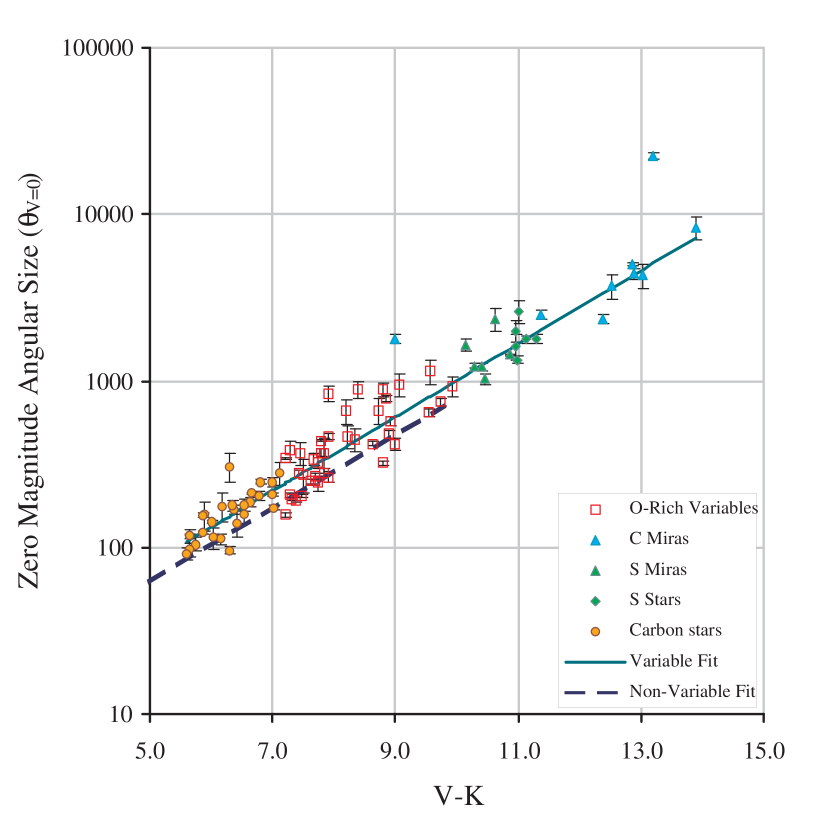
Figure 2: The $\theta_{V=0}$ zero magnitude angular size versus $V-K$ color for evolved stars, including carbon stars, S stars, all types of Mira variables, and non-Mira variables. The solid upper line is the fit line for these objects, and the dashed lower line is the fit line for the giants and supergiants from Figure 1.

The relationship appears valid over a $V-K$ range of 2.0 to 8.0. Blueward of $V-K=2.0$, the subsample is too small ($N=3$) to confidently indicate whether or not the fit is valid, in spite of the goodness of fit for the whole subsample. The same is true redward of $V-K=8.0$. Also, for stars redward of approximately $V-K=8$, care must be taken to exclude variable stars (both semiregular and Miras). The data points and the fit noted above may be seen in Figure 1; $\theta_{V=0}$ and standard deviation by $V-K$ bin is given in Table 1. The Miras are plotted separately in Figure 2 and will be discussed below.

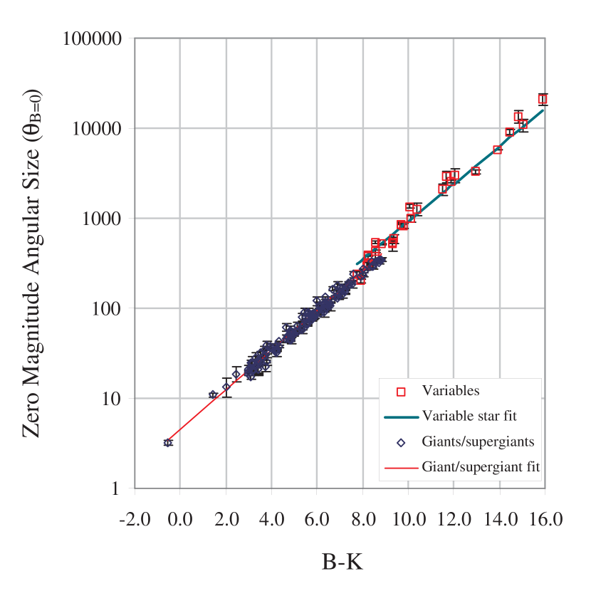
Figure 3: The $\theta_{B=0}$ zero magnitude angular size versus $B-K$ color for giant/supergiant stars and evolved stars, which includes Mira variables, S stars, carbon stars, and non-Mira variables. The upper line is the fit line for the evolved stars, the lower line is the fit line for the giants and supergiants.

For $B-K$ between 3.0 and 7.5, the relationship exhibits a similar if not slightly superior validity. As with the $V-K$ color, the relationship appears to be valid down blueward of the short edge of that range, down to $B-K=-1$, but the data are sparse. Redward of $B-K=7.5$, the relationship also exhibits potential confusion with the Mira variable stars, although there appears to be less degeneracy, but this is possibly due to a lesser availability of $B$ band data on these very red sources. The data points and the fit noted above may be seen in Figure 3; $\theta_{B=0}$ and standard deviation by $B-K$ bin is given in Table 2.

The potential misclassification of more evolved sources such as carbon stars and variables (Miras or otherwise) as normal giant and supergiant stars is a significant secondary consideration. For the dimmer sources for which little data is available, non-classification is perhaps the more appropriate term. What is reassuring with regards to the issue of classification errors is that the robust relationships between $(\theta_{V=0},V-K)$ and $(\theta_{B=0},B-K)$ are valid for stars of luminosity class I, II, and III, and that the more evolved stars occupy a redder range of $B-K$ and $V-K$ colors (cf. §3.2). Since the $\theta_{V=0}$ and $\theta_{B=0}$ relationships are insensitive to errors in luminosity class, this method is more robust than the linear radius-distance method, particularly for those stars in the $2.0<V-K<6.0$ and $3.0<B-K<7.5$ ranges, where few if any stars of significant variability exist. This relationship is also considerably easier to employ than the method of blackbody fits.

3.2 Evolved Sources: Variable Stars

By examining the 2.2 $\mu$m angular sizes for the 87 observations of 65 semiregular variables, Mira variables and carbon stars (broadly classified here as ‘variable stars’) found in the literature, we can establish a relationship between $V=0$ zero magnitude angular size and $V-K$ color:

$$\theta_{V=0}=10^{0.789\pm 0.119+0.218\pm 0.014\times(V-K)}.$$ (4)

The rms error associated with this fit is 26%. The data points and the fit noted above may be seen in Figure 3. Similarly, for $B-K$ color, 19 evolved sources had available photometry for 29 angular size observations, resulting in the following fit:

$$\theta_{B=0}=10^{0.840\pm 0.096+0.211\pm 0.008\times(B-K)},$$ (5)

with a rms error of 20%.

For the variable stars, the relationship appears valid over $V-K$, $B-K$ ranges of 5.5 to 13.0 and 9.0 to 16.0, respectively. Redward of $V-K=13$, the sample is too small ($N=3$) to confidently indicate whether or not the fit is valid, in spite of the goodness of fit for the general sample. It is interesting to note that the slope of the fits for the variable stars and for the giant/supergiant stars is statistically identical for both $V-K$ and $B-K$ colors; only the intercepts are different. This corresponds to a $\theta_{V=0}$ size factor of $1.40\pm 0.15$ between the smaller normal and and the larger variable stars for a given $V-K$ color, and a corresponding $\theta_{B=0}$ size factor of $1.34\pm 0.21$.

3.3 Main Sequence Stars

By examining the objects in the Fracassini catalog (1988; specifically, many objects from Hanbury Brown et al. 1974), there appears to be similar relationships between the $V-K$ & $B-K$ colors, and $\theta_{V=0}$ & $\theta_{B=0}$ angular sizes. The sample set of stars with adequate photometry is unfortunately limited to 11 objects. However, the Hanbury Brown objects and the Sun are measured with high accuracy and allow for accurate calibration of the stellar zero magnitude angular sizes in the ranges of $-0.4<V-K<+1.5$ and $-0.6<B-K<+2.0$. Limiting the fit analysis to the robust measurements from Hanbury Brown and for the sun, the relationships between the colors and their zero magnitude angular sizes are

$$\theta_{V=0}=10^{0.500\pm 0.023+0.264\pm 0.012\times(V-K)}\textrm{,}$$ and (6)

$$\theta_{B=0}=10^{0.500\pm 0.012+0.290\pm 0.016\times(B-K)}.$$ (7)

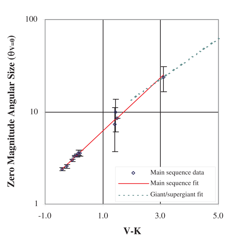
Figure 4: The $\theta_{V=0}$ zero magnitude angular size versus $V-K$ color for main sequence stars. The diamonds and solid line are the data points and fit for B, A, and G type stars, respectively; the dotted line is the fit for luminosity class I, II, and III stars.

The resulting rms errors are only 2.2% for both the $V-K$ and $B-K$ relationships. The $\theta_{V=0}$ versus $V-K$ data for these objects are plotted in Figure 4; the $\theta_{B=0}$ versus $B-K$ data are similar in appearance and will not be plotted. The relationship holds not only for the B and A type objects in the $-0.5<V-K<+0.5$ range, but also for the Sun at $V-K\approx 1.5$. Also plotted is the fit for giants and supergiants, which has a slightly different slope; the two fits are shown intersecting at $V-K\approx 2.5$, although due to poor sampling in this region it is unclear how (or if) the two functions truly join.

3.4 Analysis of Errors

As was given in §3.1, the rms fractional error between the measured and predicted values for $\theta_{V=0}$ versus $V-K$ for giants and supergiants is ${(\Delta\theta_{V=0}/\theta_{V=0})_{rms}}=11.7\%$. There are three components of this error: (1) Angular size errors, (2) Errors in $V-K$, and (3) Deviations in the relationship due to unparameterized phenomena, which shall be broadly labeled ‘natural dispersion’ in the relationship and will be discussed in more detail below. For the first component, the rms fractional error of the 163 measured $\theta$ values found in the literature is $(\Delta\theta/\theta)_{rms}=6.9\%$. For the photometry, given the heterogeneous sources, we estimate that the $V$ and $K$ photometry will have errors between 0.1 and 0.2 magnitudes (resulting in $V-K$ color errors of 0.14 to 0.28 magnitudes), which would result in an size error of 3.1-6.3%. Finally, subtracting these two sources of measurement error in quadrature from the measured dispersion, a natural dispersion in the relationship between 7.0 and 8.9% remains. A similar analysis for the giant/supergiant $\theta_{B=0}$ versus $B-K$ results in $(\Delta\theta/\theta)_{rms}=7.0\%$ for the 136 observations, indicating of 5.2-7.6% of natural dispersion. For both of these relationships, the natural dispersion is a factor as significant as the errors in angular size, and potentially the dominant factor.

For the main sequence stars, the errors in angular size for both colors were $(\Delta\theta/\theta)_{rms}=4.5\%$; the errors in photometry were expected to be no different than the giant/supergiant stars, at 0.1-0.2 magnitudes per photometric band. The main sequence stars exhibited no measureable levels of natural dispersion, being able to fully account for the observed rms spread in both the $V-K$ and $B-K$ relationships with angular size or color errors.

For the variable stars, the difficulties in obtaining contemporaneous photometry result in larger measurement error, despite steps taken to ensure epoch-dependent observations. As such, the errors are expected to be between 0.2 and 0.4 magnitudes for the individual $V$ and $K$ measurements. The resulting characterization of natural dispersion of 20-23% for the $V-K$ relationship, and 12-16% for $B-K$, dominating the angular size dispersion of $(\Delta\theta/\theta)_{rms}=10\%$ for both colors.

The specific nature of the natural dispersion term in the rms error is potentially due to stellar surface properties that affect current one-dimensional angular size determination techniques. The limited observations of individual objects with two-dimensional and more complete spatial frequency coverage have indicated asymmetries in stellar atmospheres that could potentially affect size determinations from both interferometric and lunar occultations. Early measurements of this nature were detection of asymmetries in the envelope of $o$ Cet with speckle interferometry (Karovska et al. 1991). Direct imaging of the surface of $\alpha$ Ori has provided evidence of a large hot spot on that supergiant’s surface (Gilliland & Dupree 1996). More recently, similar evidence for aspheric shapes of other Miras has been obtained, also with HST (Lattanzi et al. 1997), and evidence for more complicated morphologies in the structure of the M5 supergiant VY CMa in the near-IR has been obtained using nonredundant aperture masking on Keck 1 (Monnier et al. 1999, Tuthill et al. 1999). Various atmospheric phenomena, such as nonradial pulsations, spots on the stellar surface, and rotational distortion of the stellar envelope, potentially explain these observations. The progressive increase along stellar evolutionary states in observed natural dispersion from undetectable levels with the main sequence stars to dominant levels with the most evolved sources is consistent with the onset of these phenomena more significantly associated with extended atmospheres.

Interstellar Extinction. A brief discussion of the potential impact of interstellar extinction upon the results presented herein is warranted. The empirical reddening determination made by Mathis (1980), which agrees very well with van de Hulst’s theoretical reddening curve number 15 (see Johnson 1968), predicts that $A_{K}=0.11A_{V}$. From that relative reddening value, the effect of interstellar reddening upon the various angular size expressions may be derived to be:

$${\theta_{V=0}}^{\prime}=\theta_{V=0}\times 10^{0.225\times[{(V-K)}^{\prime}-(V-K)]}\textrm{,}$$ and (8)

$${\theta_{V=0}}^{\prime}=\theta_{V=0}\times 10^{0.218\times[{(V-K)}^{\prime}-(V-K)]}.$$ (9)

Comparison of the slopes of equations (2) and (3) with (8) and (9) demonstrates that the angular size predictions for giant and supergiant stars are almost wholly unaffected by the effects of interstellar extinction: any apparent reddening of a star’s $V-K$ or $B-K$ color is accompanied by an increase in the associated zero magnitude angular size, along the slope of the predict lines. This effect is independent of the absolute amount of reddening encountered by a star, since it is a relative effect between the two bandpasses of a given color.

For main sequence stars, the slopes between the predict lines and reddening effect indicates a gradual underestimation in actual stellar size as reddening increases. Based upon typical reddening values of $A_{V}=0.8-1.9$ mag/kpc, a 2.2% effect (consistent with the expected level of error in the angular size prediction) will be present for stars with $A_{V}=0.18$, corresponding to distances between 95 and 225 pc. For the variable stars, the slopes also skew, but slightly less so, and in the opposite sense: the gradual trend will be to overestimate sizes for reddened sources. A 20% effect for these stars will be present for stars at $A_{V}=16.9$, corresponding to distances between 8.8 and 21 kpc - clearly not a significant factor for the current accuracy of either the $V-K$ or $B-K$ relationship.

4 Comparison of the Various Methods

Previous approaches for estimating angular sizes have included estimates of stellar linear size coupled with distance measurements or estimates, and the extraction of angular sizes by treating the objects as blackbody radiators. The release of the Hipparcos catalog (Perryman et al. 1997), with its parallax data, has increased the utility of the first method. Spectral type and $V-K$ color have been explored as indicators of intrinsic linear size for giant stars (van Belle et al. 1999a). Similarly, spectral type can be used to predict linear size for main sequence stars (Allen 1973), although this relationship appears to be poorly characterized. There does not appear to be a $V-K$-linear radius relationship presented for these stars in the literature, which would be consistent with both photometric bands being on the Rayleigh-Jeans tail of the blackbody curve for these hotter ($T>6000K$) objects. The relative errors for predicting stellar angular diameters were calculated as discussed in §3 for the stars in the §2 sample using these alternative methods, and are summarized in Table 3. For all of the stars in question, deriving an apparent angular size from a $\theta_{V=0}$ or $\theta_{B=0}$ zero magnitude angular size delivers the best results.

5 Conclusion

The new approach of establishing the $\theta_{V=0}$ and $\theta_{B=0}$ zero magnitude angular sizes appears to be an unrecognized yet powerful tool for predicting the apparent angular sizes of stars of all classes. The very modest data requirements of this method make it an ideal tool for quantification of this fundamental stellar parameter.

Table 1: Zero Magnitude Angular Size for Giants and Supergiants as a Function of $V-K$ Color

	Normal Giants and Supergiants					Variables
$V-K$			Std.					Std.
Center	$N$	$\overline{\theta}_{V=0}$	Dev.	Fit		$N$	$\overline{\theta}_{V=0}$	Dev.	Fit	Ratio
-0.5	1	3.4		3.7		0
0.0	0			4.8		0
0.5	0			6.2		0
1.0	1	9.1		8.0		0
1.5	2	11.6	1.8	10.3		0
2.0	9	13.9	1.7	13.3		0
2.5	17	16.7	3.1	17.2		0
3.0	12	20.5	3.1	22.3		0
3.5	20	27.2	4.4	28.7		0
4.0	21	37.8	4.4	37.1		0
4.5	15	47.0	5.7	47.9		0
5.0	18	58.2	5.9	61.9		0
5.5	15	80.3	13.9	79.9		4	105	13	103	$1.31\pm 0.28$
6.0	7	102.7	13.3	103.1		7	140	25	132	$1.37\pm 0.30$
6.5	5	122.9	18.3	133.1		9	181	57	170	$1.47\pm 0.51$
7.0	9	159.6	23.5	171.9		8	233	60	220	$1.46\pm 0.43$
7.5	6	197.0	21.0	221.9		14	270	62	283	$1.37\pm 0.35$
8.0	0			286.6		9	461	184	365
8.5	1	355.4		370.0		4	605	217	470	$1.70\pm 0.61$
9.0	1	431.0		477.7		7	631	245	605	$1.46\pm 0.57$
9.5	0					3	841	259	780
10.0	0					2	1286	511	1005
10.5	0					4	1456	604	1295
11.0	0					6	1795	465	1669
11.5	0					2	2146	498	2150
12.0	0					0
12.5	0					2	3033	965	3569
13.0	0					0
13.5	0					0
14.0	0					1	8323		7635

Note. — The number of stars $N$, average size $\theta_{V=0}$, and standard deviation for each bin is given for both normal giant and supergiant stars, and for variables, inclusive of Miras, semi-regulars, and carbon stars. The fits given are those discussed in §3; the ratios given are the average $\theta_{V=0}$ size ratios for those $V-K$ bins where values exist for both giant/supergiant stars and variables. In general, the variable stars have a $\theta_{V=0}$ size that is $1.44\pm 0.15$ larger than their ‘normal’ star counter parts for a given $V-K$ color.

Table 2: Zero Magnitude Angular Size for Giants and Supergiants as a Function of $B-K$ Color

	Normal Giants and Supergiants					Variables
$B-K$			Std.					Std.
Bin Center	$N$	$\overline{\theta}_{B=0}$	Dev.	Fit		$N$	$\overline{\theta}_{B=0}$	Dev.	Fit	Ratio
-0.5	1	3.2		3.5		0
0.0	0			4.5		0
0.5	0			5.8		0
1.0	0			7.5		0
1.5	1	10.9		9.7		0
2.0	1	13.6		12.5		0
2.5	1	18.7		16.1		0
3.0	10	21.4	2.7	20.7		0
3.5	13	26.2	4.2	26.7		0
4.0	11	34.5	3.6	34.4		0
4.5	6	47.2	8.2	44.3		0
5.0	15	51.9	5.3	57.1		0
5.5	14	74.9	11.5	73.6		0
6.0	18	89.5	12.0	94.8		0
6.5	12	114.4	19.3	122.1		0
7.0	13	151.5	15.9	157.4		0
7.5	6	196.1	21.3	202.8		0
8.0	4	248.4	23.2	261.2		6	304	75	352	$1.23\pm 0.32$
8.5	7	315.6	21.8	336.6		3	451	84	447	$1.43\pm 0.28$
9.0	2	344.2	5.5	433.7		1	520		569
9.5	0					5	669	164	723
10.0	0					3	1057	273	919
10.5	0					1	1270		1169
11.0	0					0
11.5	0					2	2501	561	1889
12.0	0					2	2802	316	2402
12.5	0					0
13.0	0					1	3302		3883
13.5	0					0
14.0	0					1	5797		6276
14.5	0					1	9077		7979
15.0	0					2	12161	1755	10144

Note. — The number of stars $N$, average size $\theta_{B=0}$, and standard deviation for each bin is given for both normal giant and supergiant stars, and for variables, inclusive of Miras, semi-regulars, and carbon stars. The fits given are those discussed in §3; the ratios given are the average $\theta_{B=0}$ size ratios for those $B-K$ bins where values exist for both giant/supergiant stars and variables. In general, the variable stars have a $\theta_{B=0}$ size that is $1.34\pm 0.21$ larger than their ‘normal’ star counter parts for a given $B-K$ color.

Table 3: Comparison of the Various Angular Size Prediction Methods

Method			Error	Notes
Main Sequence Stars
	Linear Radius by Spectral Type		25%
	Linear Radius by $V-K$ Color		N/A
	Angular Size by BBR Fit		13%
	$V=0$ Angular Size by $V-K$ Color		2.2%
	$B=0$ Angular Size by $B-K$ Color		2.2%
Giant, Supergiant Stars
	Linear Radius by Spectral Type		22%	Giants only
	Linear Radius by $V-K$ Color		22%	Giants only
	Angular Size by BBR Fit		18%
	$V=0$ Angular Size by $V-K$ Color		11.7%
	$B=0$ Angular Size by $B-K$ Color		10.8%
Variable Stars
	$V=0$ Angular Size by $V-K$ Color		26%
	$B=0$ Angular Size by $B-K$ Color		20%

Note. — Errors given above are percentage errors relative to the value predicted by each method.

References

- (1) Allen, C.W. 1973, Astrophysical Quantities, (London: Athlone Press)
- (2) Barnes, T.G., & Evans, D.S. 1976, MNRAS, 174, 489
- (3) Barnes, T.G., Evans, D.S., & Moffett, T.J. 1978, MNRAS, 183, 285
- (4) Barnes, T.G., Evans, D.S., & Parsons, S.B. 1976, MNRAS, 174, 503
- (5) Beichman, C.A., Chester, T.J., Skrutskie, M., Low, F.J., & Gillett, F. 1998, PASP, 110, 480
- (6) Blackwell, D.E., & Lynas-Gray, A.E. 1998, A&AS, 129, 505
- (7) Cohen, M., Witteborn, F.C., Carbon, D.F., Davies, J.K., Wooden, D.H., & Bregman, J.D. 1996, AJ, 112, 2274
- (8) Di Benedetto, G.P. 1993, A&A, 270, 315
- (9) Di Giacomo, A., Lisi, F., Calamai, G., & Richichi, A. 1991, A&A, 249, 397
- (10) Dyck, H.M., Benson, J.A., van Belle, G.T., & Ridgway, S.T. 1996a, AJ, 111, 1705
- (11) Dyck, H.M., van Belle, G.T., & Benson, J.A. 1996b, AJ, 112, 294
- (12) Dyck, H.M., van Belle, G.T., & Thompson, R.R. 1998, AJ, 116, 981
- (13) Egret, D., Wenger, M., & Dubois, P. 1991, in Databases and On-line Data in Astronomy, ed. Albrecht, M.A. & Egret, D. (Dordrecht, Kluwer), p. 79
- (14) Epchtein, N. 1997, in The Impact of Large Scale Near-infrared Surveys, ed. Garzon, F., Epchtein, N., Omont, A., Burton, W.B., & Persi, P.(Dordrecht: Kluwer)
- (15) Fracassini, M., Pasinetti-Fracassini, L.E., Pastori, L., & Pironi, R. 1988, Bull. D’Inf. Cent. Donnees Stellaires, 35, 121
- (16) Genova, F., Bonnarel, F., Bartlett, J.G., Dubois, P., Egret, D., Jasniewicz, G. et al. 1997, Baltic Astronomy, 6, 192
- (17) Gezari, D.Y., Pitts, P.S., & Schmitz, M. 1997, Catalog of Infrared Observations, Edition 4, unpublished but available online at http://adc.gsfc.nasa.gov/
- (18) Gezari, D.Y., Schmitz, M., Pitts, P.S., & Mead, J.M. 1993, Catalog of Infrared Observations, 3rd Edition, NASA Reference Publication 1294
- (19) Gilliland, R.L., & Dupree, A.K. 1996, ApJ, 463, 29
- (20) Gunther, J. 1996, JAVSO, 24, 17
- (21) Hanbury Brown, R., Davis, J., Lake, R.J.W., & Thompson, R.J. 1974, MNRAS, 167, 475
- (22) Hutter, D.J., Johnston, K.J., Mozurkewich, D., Simon, R.S., Colavita, M.M., Pan, X.P. et al. 1989, ApJ, 340, 1103
- (23) Johnson, H.L., 1968, in Nebulae and Interstellar Matter, edited by B.M. Middlehurst and L.H. Aller (University of Chicago Press, Chicago), Chap. 5
- (24) Karovska, M., Nisenson, P., Papaliolios, C., & Boyle, R. P. 1991, ApJ, 374, 51
- (25) Lattanzi, M.G., Munari, U., Whitelock, P.A., & Feast, M.W. 1997, ApJ, 485, 328
- (26) Mathis, J.S., 1980, ARA&A, 28, 37
- (27) Mermilliod, J.-C., Mermilliod, M., & Hauck, B. 1997, A&AS, 124, 349
- (28) Monnier, J.D., Tuthill, P.G., Lopez, B., Cruzalebes, P., Danchi, W.C., & Haniff, C.A. 1999, ApJ, 512, 351
- (29) Mozurkewich, D. 1999, private communication
- (30) Mozurkewich, D., Johnston, K.J., Simon, R.S., Bowers, P. F., Gaume, R., Hutter, D.J. et al. 1991, AJ, 101, 2207
- (31) Nordgren, T. 1999, private communication
- (32) Percy, J. R., Mattei, J. A. 1993, Ap&SS, 210, 137
- (33) Perrin, G., Coud du Foresto, V., Ridgway, S.T., Mariotti, J.-M., Traub, W.A., Carleton, N.P., & Lacasse, M.G. 1998, A&A, 331, 619
- (34) Perryman, M.A.C., Lindegren, L., Kovalevsky, J., Hog, E., Bastian, U., Bernacca, P.L. et al. 1997, A&A, 323, L49
- (35) Press, W.H., Teukolsky, S.A., Vetterling, W.T., & Flannery, B.P. 1992, Numerical Recipes in C (Port Chester, NY: Cambridge University Press), 689
- (36) Richichi, A., Salnari, P., & Lisi, F. 1988, ApJ, 326, 791
- (37) Richichi, A., Lisi, F., & Calamai, G. 1991, A&A, 241, 131
- (38) Richichi, A., Lisi, F., & Di Giacomo, A. 1992, A&A, 254, 149
- (39) Richichi, A., Di Giacomo, A., Lisi, F., & Calamai, G. 1992, A&A, 265, 535
- (40) Richichi, A., Chandrasekhar, T., Lisi, F., Howell, R.R., Meyer, F., Rabbia, Y. et al. 1995, A&A, 301, 439
- (41) Richichi, A., Ragland, S., & Fabbroni, L. 1998a, A&A, 330, 578
- (42) Richichi, A., Stecklum, B., Herbst, T.M., Lagage, P.-O., & Thamm, E. 1998b, A&A, 334, 585
- (43) Richichi, A., Ragland, S., Stecklum, B., & Leinert, C. 1998c, A&A, 338, 527
- (44) Richichi, A., Fabbroni, L., Ragland, S., & Scholz, M. 1999, A&A, 344, 511
- (45) Ridgway, S.T., Wells, D.C., & Carbon, D.F. 1974, AJ, 79, 1079
- (46) Ridgway, S.T., Wells, D.C., & Joyce, R.R. 1977, AJ, 82, 414
- (47) Ridgway, S.T. 1977, AJ, 82, 511
- (48) Ridgway, S.T., Wells, D.C., Joyce, R.R., & Allen, R.G. 1979, AJ, 84, 247
- (49) Ridgway, S.T., Jacoby, G.H., Joyce, R.R., & Wells, D.C. 1980a, AJ, 85, 1496
- (50) Ridgway, S.T., Joyce, R.R., White, N.M., & Wing, R.F., 1980b, ApJ, 235, 126
- (51) Ridgway, S.T., Jacoby, G.H., Joyce, R.R., Siegel, M.J., & Wells, D.C. 1982a, AJ, 87, 680
- (52) Ridgway, S.T., Jacoby, G.H., Joyce, R.R., Siegel, M.J., & Wells, D.C. 1982b, AJ, 87, 808
- (53) Ridgway, S.T., Jacoby, G.H., Joyce, R.R., Siegel, M.J., & Wells, D.C. 1982b, AJ, 87, 1044
- (54) Schmidtke, P.C., Africano, J.L., Jacoby, G.H., Joyce, R.R., & Ridgway, S.T. 1986, AJ, 91, 961
- (55) Tuthill, P.G., Haniff, C.A., Baldwin, J.E. 1999, MNRAS, 306, 353
- (56) van Belle, G.T., Dyck, H.M., Benson, J.A., & Lacasse, M.G. 1996, AJ, 112, 2147
- (57) van Belle, G.T., Dyck, H.M., Thompson, R.R., Benson, J.A., & Kannappan, S.J. 1997, AJ, 114, 2150
- (58) van Belle, G.T., Lane, B.F., Thompson, R.R., Boden, A.F., Colavita, M.M., Dumont, P.J. et al. 1999a, AJ, 117, 521
- (59) van Belle, G.T., Thompson, R.R., & Creech-Eakman, M. 1999b in preparation
- (60)