Tropospheric Phase Calibration in Millimeter Interferometry

Abstract

We review millimeter interferometric phase variations caused by variations in the precipitable water vapor content of the troposphere, and we discuss techniques proposed to correct for these variations. We present observations with the Very Large Array at 22 GHz and 43 GHz designed to test these techniques. We find that both the Fast Switching and Paired Array calibration techniques are effective at reducing tropospheric phase noise for radio interferometers. In both cases, the residual rms phase fluctuations after correction are independent of baseline length for b $>$ b_eff. These techniques allow for diffraction limited imaging of faint sources on arbitrarily long baselines at mm wavelengths.

We consider the technique of tropospheric phase correction using a measurement of the precipitable water vapor content of the troposphere via a radiometric measurement of the brightness temperature of the atmosphere. Required sensitivities range from 20 mK at 90 GHz to 1 K at 185 GHz for the MMA, and 120 mK for the VLA at 22 GHz. The minimum gain stability requirement is 200 at 185 GHz at the MMA assuming that the astronomical receivers are used for radiometry. This increases to 2000 for an uncooled system. The stability requirement is 450 for the cooled system at the VLA at 22 GHz. To perform absolute radiometric phase corrections also requires knowledge of the tropospheric parameters and models to an accuracy of a few percent. It may be possible to perform an ‘empirically calibrated’ radiometric phase correction, in which the relationship between fluctuations in brightness temperature differences with fluctuations in interferometric phases is calibrated by observing a strong celestial calibrator at regular intervals. A number of questions remain concerning this technique, including: (i) over what time scale and distance will this technique allow for radiometric phase corrections when switching between the source and the calibrator? and (ii) how often will calibration of the T${}_{\rm B}^{\rm rms}$ - $\phi_{rms}$ relationship be required?

1 Introduction

The most important difference between mm and cm interferometry is the effect of the troposphere at mm wavelengths. The optical depth of the troposphere becomes significant below 1 cm, leading to increased system temperatures due to atmospheric emission, and increased demands on gain calibration due to variable opacity (Yun et al., 1998, Kutner and Ulich 1981). Even more dramatic is the effect of the troposphere on interferometer phases. Variations in the tropospheric water vapor column density lead to variations in electronic pathlength, and hence variations in interferometric phase. This can cause loss of amplitude of the cross correlations, or ‘visibilities’, over the integration time (‘coherence’), reduced spatial resolution (‘seeing’), and pointing errors (‘anomalous refraction’).

Until recently, mm interferometric arrays have been restricted to maximum baselines of a few hundred meters. Diffraction limited resolution images at mm wavelengths can be made on such baselines, since the tropospheric phase fluctuations on such baselines at good observatory sites are typically one radian or less under good weather conditions. However, many existing mm arrays are expanding to baselines of 1 km or more, and the planned large millimeter array facility at the Chajnantor site in Chile will have baselines as long at 10 km. Even at this premium site, phase fluctuations due to the troposphere will be larger than 1 radian at 230 GHz on these baselines, except under the best weather conditions. Hence, tropospheric seeing will preclude diffraction limited resolution imaging at frequencies of 230 GHz for arrays larger than about 1 km, even at the best possible sites, if no corrections are made for tropospheric phase noise. At higher frequencies, the maximum baselines which would permit uncorrected observations would be even shorter.

In this paper we review the theory of tropospheric phase noise in mm interferometry, along with examples showing tropospheric induced phase fluctuations and their effect on images made with interferometric arrays. We then consider three techniques for reducing tropospheric phase noise: (i) Fast Switching phase calibration, (ii) Paired Array phase calibration, and (iii) radiometric phase calibration. The first two techniques entail using celestial calibration sources near the target source, with either a calibration cycle time fast enough to ‘stop’ the troposphere (Fast Switching), or by using some of the antennas as a tropospheric ‘calibration array’ (Paired Array). We present extensive observational data using the Very Large Array (VLA) in Socorro, NM, USA, at 22 GHz and 43 GHz designed to test the efficacy of these first two techniques on baselines longer than a few km.

The radiometric phase correction technique entails real-time estimation of the precipitable water vapor content along each antenna’s line of sight through the troposphere via a radiometric measurement of the brightness temperature of the atmosphere above each antenna. A number of issues are addressed, including: (i) the required radiometric sensitivity as a function of frequency and site quality, (ii) the constraints on ancillary data, such as atmospheric data and models, in order to perform an absolute radiometric phase correction, and (iii) the limitations to making radiometric phase corrections by calibrating the relationship between brightness temperature fluctuations and interferometric phase using celestial sources.

2 A General Description of the Troposphere and the Mean Tropospheric Effect on Interferometric Phase

The troposphere is the lowest layer of the atmosphere, extending from the ground to the stratosphere at an elevation of 7 km to 10 km. The temperature decreases with altitude in this layer, clouds form, and convection can be significant (Garratt 1992). The troposphere is composed predominantly of N₂, O₂, plus trace gases such as water vapor, N₂O, and CO₂, plus particulates such as liquid water and dust in clouds. The troposphere becomes increasingly opaque with increasing frequency, mostly due to absorption by O₂ and H₂O.

Figure 1 shows models of the atmospheric transmission at cm and mm wavelengths for the VLA site at 2150 m altitude, and the planned millimeter array (MMA) site in Chile at 4600 m altitude (Holdaway and Pardo 1997, Liebe 1989). The plot shows a series of strong absorption lines including the water lines at 22 GHz and 183 GHz, and the O₂ lines at 60 GHz and 118 GHz, plus a systematic decrease in the transmission with increasing frequency between the lines. This ‘pseudo-continuum’ opacity is due to the sum of the pressure broadened line wings of a multitude of sub-mm and IR lines of water vapor. The plot for the MMA site at Chajnantor in Chile includes the typical value for the column density of precipitable water vapor, w_∘ = 1 mm, while the water vapor column for the VLA site is assumed to be w_∘ = 4 mm, where precipitable water vapor (PWV) = the depth of the water vapor if converted to the liquid phase. Figure 2 shows the relative contributions from water vapor and dry air (O₂ plus other trace gases) for the VLA site. Below 130 GHz, both O₂ and H₂O contribute significantly to the optical depth. Above 130 GHz, H₂O dominates the optical depth.

The troposphere has a non-unit refractive index, $n$. The refractive index is defined by the phase change experienced by an electromagnetic wave, $\phi_{e}$, propagating over a physical distance, D:

$$\phi_{e}={{2\pi}\over{\lambda}}\times n\times\rm D,$$

or, in terms of ‘electrical pathlength’, L_e:

$$\rm L_{e}=\lambda\times{{\phi_{e}}\over{2\pi}}={\it n}\times D$$

The refractive index of air is non-dispersive (ie, independent of frequency) except near the strong resonant water and O₂ lines, and is typically given as a difference with respect to vacuum ($n_{vacuum}$ $\equiv$ 1), in parts per million, $N$, as (Waters 1976):

$$N\equiv(n-1)\times 10^{6}$$

The index of refraction of air is typically separated into the dry air component, $N_{d}$, and the water vapor component, $N_{wv}$. These terms behave as (Waters 1976, Bean and Dutton 1968):

$$N_{d}=2.2\times 10^{5}\times\rho_{tot}$$

$$N_{wv}=1.7\times 10^{9}\times{{\rho_{wv}}\over{\rm T_{\rm atm}}}$$

where $\rho_{tot}$ is the total mass density in gm cm^-3, and $\rho_{wv}$ is the water vapor mass density. The inverse dependence on temperature for $N_{wv}$ is due to the increased effect of collisions on the (mis-)alignment of the permanent electric dipole moments of the water molecules with increasing temperature (Waters 1976, Bean and Dutton 1968). A detailed derivation of these relationships can be found in Thompson, Moran, and Swenson (1986).

For water vapor alone, it can be shown that $\rho_{wv}$ = ${\rm w}\over{\rm D}$. Using the equations above then leads to the relationship between the electrical pathlength, L_e, and the precipitable water vapor column, w:

$$\rm L_{e}=1.7\times 10^{3}{{w}\over{T_{\rm atm}}}\approx 6.3\times\rm w$$

or:

$$\phi_{e}\approx{{12.6\pi}\over{\lambda}}\times\rm w$$ (1)

for T_atm $\approx$ 270 K. This relation between electrical pathlength and precipitable water vapor column has been verified experimentally for a number of atmospheric conditions (Hogg, Guiraud, and Decker 1981).

3 Phase Variations due to the Troposphere

Variations in precipitable water vapor lead to variations in the effective electrical path length, corresponding to variations in the phase of an electromagnetic wave propagating through the troposphere (Tatarskii 1978). Such variations are seen as ‘phase noise’ by radio interferometers. Since the troposphere is non-dispersive, the phase contribution by a given amount of water vapor increases linearly with frequency (except in the vicinity of the strong water lines). Hence, tropospheric phase variations are most prominent for mm and sub-mm interferometers, and can be the limiting factor for the coherence time and spatial resolution of mm interferometers (Hinder and Ryle 1971, Lay 1997, Wright 1996).

The standard model for tropospheric phase fluctuations involves variations in the water vapor column density in a turbulent layer in the troposphere with a mean height, h_turb, and a vertical extent, W, which moves at some velocity, v_a. This model includes the ‘Taylor hypothesis’, or ‘frozen screen approximation’, which states that: ‘if the turbulent intensity is low and the turbulence is approximately stationary and homogeneous, then the turbulent field is unchanged over the atmospheric boundary layer time scales of interest and advected with the mean wind’ (Taylor 1938, Garratt 1992). Under this assumption one can relate temporal and spatial phase fluctuations with a simple Eulerian transformation between baseline length, b, and v_a:  b = v_a$\times$time. In the following sections we adopt a value of v_a = 10 m s^-1. This process is shown schematically in Figure 3.

A demonstration of tropospheric phase fluctuations is shown in Figure 4 for observations made with the VLA at 22 GHz. The VLA is an aperture synthesis array comprised of 27 parabolic antennas of 25m diameter, operating at frequencies from 75 MHz to 50 GHz (Napier, Thompson, and Ekers 1983). The antennas are situated in a ‘Y’ pattern, along three arms situated north, southwest, and southeast. The maximum physical baseline in the largest configuration is 33 km. The complex cross correlations of the electric fields measured at each antenna are calculated between all pairs of antennas (‘interferometers’) as a function of time. The Fourier transform of these measurements of the spatial coherence function of the electric field then gives the sky brightness distribution (Clark 1998).

For these observations, two subarrays were employed, one observing the celestial calibrator 0423+418, and the second observing the calibrator 0432+416. The sub-arrays were ‘inter-laced’, meaning that every second antenna along each arm of the array observed a given source. Antenna-based phase and amplitude solutions were derived from the data in each sub-array using self-calibration with an averaging time of 30 sec (Cornwell 1998). Figure 4 shows the antenna-based phase solutions from two pairs of neighboring antennas along the southwest arm. The antennas at stations W16 and W4 were observing 0423+418 while the antennas at W18 and W6 were observing 0432+416. For adjacent pairs of antennas (W16-W18 and W6-W4) the temporal variations in the phase track each other closely. This close relationship for phase variations between neighboring antennas in the two different subarrays is the signature that the phase variations are primarily tropospheric in origin, and are correlated on relevant timescales and baseline lengths.

An important aspect of tropospheric phase fluctuations arising from the Taylor hypothesis is the relationship between the amplitude of the fluctuations and the time scale: large amplitude fluctuations occur over long periods and are partially correlated between antennas, while small amplitude fluctuations occur over short periods and are uncorrelated between antennas, depending on the baseline length. This effect can be seen in Figure 4 by the fact that the antennas at the outer stations (W14 and W16) show larger amplitude fluctuations relative to the inner stations (W4 and W6). This occurs because the antenna-based phase solutions for each subarray are referenced to antennas at the center of the array, such that the reference antennas are within about 250 m of W4 and W6, but are separated from W16 and W14 by about 2000 m.

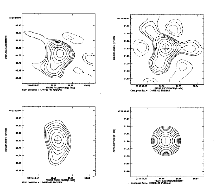
Figure 5: VLA images of the celestial calibrator 2007+404 at 22 GHz with a resolution of 0.1^′′ made from observations on July 22, 1998. The tick-marks on the declination axis are separated by 50 mas. The upper two frames show ‘snap-shot’ images made from one minute of data at the beginning (left) and end (right) of the one hour observation. These data were self-calibrated with an averaging time of 30 minutes, ie. just a mean phase was removed for each half of the observation. The cross in each figure is a fiducial mark indicating the true position of the source. The lower left frame shows the image of 2007+404 made using the full hour of data with a self-calibration averaging time of 30 minutes. The lower right frame shows the same image after self-calibration with an averaging time of 30 seconds. The lower left frame has a peak surface brightness of 1.0 Jy beam^-1, and off-source rms noise of 47 mJy beam^-1, and a total flux density of 1.5 Jy. The lower right frame has a peak surface brightness of 1.6 Jy beam^-1, a noise of 5 mJy beam^-1, and a total flux density of 1.6 Jy. In all images the contour levels are a geometric progression in the square root of two, with the first level being 0.11 Jy beam^-1. Dotted contours are negative.

An example of what occurs in the image plane due to tropospheric phase fluctuations is shown in Figure 5. Observations were made of the celestial calibrator 2007+404 at 22 GHz with the VLA at a resolution of 0.1^′′ (maximum baseline = 30 km) for a period of 1 hour. The data were self-calibrated using a long solution averaging time of 30 minutes, ie. just a mean phase was removed from each half of the data. ‘Snap-shot’ images were then made from one minute of data at the beginning and end of the observation (upper left and upper right frames in Figure 5, respectively). Two important trends are apparent in these two frames. First, notice the positive-negative side-lobe pairs straddling the peak, indicative of antenna-based phase errors (Ekers 1998). These image artifacts are due to phase fluctuations which arise in small scale water vapor structures in the troposphere that are not correlated between antennas. Second, notice that the peak in each image has shifted from the true source position. This position shift is due to phase fluctuations which arise in large scale water vapor structures in the troposphere that are correlated between antennas, ie. a phase gradient across the array. These two frames are analogous to optical ‘speckle’ images, although the timescales in the radio are much longer than in the optical due to the larger spatial scales for the turbulence.

The lower left frame shows the image of 2007+404 made using the full hour of data, but with a self-calibration averaging time of 30 minutes. The source appears extended in this image. The lower right frame shows the same image after self-calibration with an averaging time of 30 seconds, and in this case the source is unresolved, ie. the source size is equivalent, within the noise, to the interferometric synthesized beam. The lower left image has a peak surface brightness of 1.0 Jy beam^-1, an off-source rms noise level of 47 mJy beam^-1, and a total flux density of 1.5 Jy. The lower right image has a peak surface brightness of 1.6 Jy beam^-1, an off-source rms noise level of 5 mJy beam^-1, and a total flux density of 1.6 Jy. Not correcting for tropospheric phase noise in the lower left frame has: (i) increased the off-source noise in the image, (ii) decreased the ‘coherence’ (ie. lowered the peak surface brightness), and (iii) degraded the resolution (‘seeing’).

The important lesson from Figure 5 is that, while tropospheric phase errors can be quantified in terms of an antenna-based phase error, the errors are partially correlated between antennas on certain spatial and temporal scales, leading to positional shifts of sources as well as the standard positive-negative side-lobe pairs. Also, it is important to keep in mind that short baselines only ‘sample’ the power in the phase screen on scales of order the baseline length.

4 Root Phase Structure Function

Tropospheric phase fluctuations are usually characterized by the spatial phase structure function, $\rm D_{\Phi}(b)$,

$$\rm D_{\Phi}(b)\equiv\langle(\Phi(x+b)-\Phi(x))^{2}\rangle,$$ (2)

where b is the distance between two antennas, $\rm\Phi(x+b)$ is the atmospheric phase measured at one antenna and $\rm\Phi(x)$ is the atmospheric phase measured at the second antenna, and the brackets represent an ensemble average. Usually in radio astronomy the ensemble average is replaced by a time average on one particular baseline. An interferometric array will sample the phase structure function at several baselines. For a single interferometer, the Taylor hypothesis (which asserts that temporal phase fluctuations are equivalent to spatial phase fluctuations) permits us to measure temporal phase fluctuations on a single baseline and translate these into the equivalent spatial phase structure function. In the following discussion we consider the square root of the phase structure function (the ‘root phase structure function’), which corresponds to the rms phase variations as a function of baseline length:

$$\rm\Phi_{rms}\equiv\sqrt{D_{\Phi}}$$

.

Kolmogorov turbulence theory (Coulman 1990) predicts a function of the form:

$$\rm\Phi_{\rm rms}(b)={K\over{\lambda_{mm}}}~{}b^{\alpha}~{}~{}deg,$$ (3)

where b is in km, and $\lambda$ is in mm. A typical value of K = 100 for the MMA site in Chajnantor under good weather conditions, and K = 300 is typical for the VLA site (Carilli, Holdaway, and Sowinski 1996, Sramek 1990).

Kolmogorov turbulence theory predicts $\alpha$ = ${1\over 3}$ for baselines longer than the width of the turbulent layer, W, and $\alpha$ = ${5\over 6}$ for baselines shorter than W (Coulman 1990). The change in power-law index at b $=$ W is due to the finite vertical extent of the turbulent layer. For baselines shorter than W the full 3-dimensionality of the turbulence is involved (thick-screen), while for longer baselines a 2-dimensional approximation applies (thin-screen). Turbulence theory also predicts an ‘outer-scale’, L_∘, beyond which the rms phase variations should not increase with baseline length (ie. $\alpha$ = 0). This scale corresponds to the largest coherent structures, or maximum correlation length, for water vapor fluctuations in the troposphere, presumably set by external boundary conditions.

Recent observations with the VLA support Kolmogorov theory for tropospheric phase fluctuations. Figure 6 shows the root phase structure function made using the BnA configuration of the VLA. This configuration has good baseline coverage ranging from 200m to 20 km, hence sampling all three hypothesized ranges in the structure function. Observations were made at 22 GHz of the VLA calibration source 0748+240. The total observing time was 90 min, corresponding to a tropospheric travel distance of 54 km, using v_a = 10 m s^-1 (see section 6.2). The open circles show the nominal tropospheric root phase structure function over the full 90 min time range. The solid squares are the rms phases after subtracting (in quadrature) a constant electronic noise term of 10^∘, as derived from the data by requiring the best power-law on short baselines. The 10^∘ noise term is consistent with previous measurements at the VLA indicating electronic phase noise increasing with frequency as 0.5^∘ per GHz (Carilli and Holdaway 1996).

The three regimes of the structure function as predicted by Kolmogorov theory are verified in Figure 6. On short baselines (b $\leq$ 1.2 km) the measured power-law index is 0.85$\pm$0.03 and the predicted value is 0.83. On intermediate baselines (1.2 $\leq$ b $\leq$ 6 km) the measured index is 0.41$\pm$ 0.03 and the predicted value is 0.33. On long baselines (b $\geq$ 6 km) the measured index is 0.1$\pm$0.2 and the predicted value is zero. The implication is that the vertical extent of the turbulent layer is:  W $\approx$ 1 km, and that the outer scale of the turbulence is:  L_∘ $\approx$ 6 km. The increase in the scatter of the rms phases for baselines longer than 6 km may be due to an anisotropic outer scale (Carilli and Holdaway 1997).

In practice, single baseline site testing interferometers tend to see values of $\alpha$ which form a continuous distribution between the theoretical thin and thick layer values of ${1\over 3}$ and ${5\over 6}$ (Holdaway et al., 1995). The distribution cuts off fairly sharply at these two theoretical values. Such a distribution could be due to the presence of both a thin turbulent layer associated with the ground or an inversion layer and a thick turbulent layer. By changing the relative weight of each of these two layers with their theoretical power law exponents, the resulting phase structure function will be very close to a power law with an exponent between the two theoretical values. Alternatively, the intermediate power law values could just reflect the transition between thin and thick turbulence.

5 Effects of Tropospheric Phase Noise

5.1 Coherence

Tropospheric phase noise leads to a number of adverse effects on interferometric observations at mm wavelengths. First is the loss of coherence of a measured visibility on a given baseline over a given averaging time due to phase variations. For a given visibility, V = V_∘e^iϕ, the effect on the measured amplitude due to phase noise in a given averaging in time is:

$$<\rm V>=\rm V_{\circ}\times<e^{i\phi}>=V_{\circ}\times e^{-\phi_{\rm rms}^{2}/2}$$ (4)

assuming Gaussian random phase fluctuations with an rms variation of $\phi_{\rm rms}$ over the averaging time (Thompson, Moran, and Swenson 1986). For example, for $\phi_{\rm rms}$ = 1 rad, the coherence is:  ${<\rm V>}\over{\rm V_{\circ}}$ = 0.60, meaning the observed visibility amplitude is reduced by 40$\%$ from the true value.

5.2 Seeing

A second effect of tropospheric phase fluctuations is to limit the spatial resolution of an observation in a manner analogous to optical seeing, where optical seeing is due to thermal fluctuations rather than water vapor fluctuations. Since interferometric phase corresponds to the measurement of the position of a point source (Perley 1998), it is clear that phase variations due to the troposphere will lead to positional variations of a source, and hence ‘smear-out’ a point source image over time (Figure 5). The magnitude of tropospheric seeing can be calculated by considering the coherence as a function of baseline length. Since the coherence decreases for longer baselines given an averaging time long compared to the array crossing time, the observed visibility amplitude decreases with increasing baseline length, as would occur if the source were resolved by the array. Using equation 3 for the root phase structure, and equation 4 for the coherence, the visibility amplitude as a function of baseline length becomes:

$$<\rm V>=V_{\circ}\times exp(-[{{K^{\prime}b^{\alpha}}\over{\lambda\sqrt{2}}}]^{2})$$ (5)

Note that the exponent must be in radians, so K^′ = K $\times$ ${2\pi}\over{360}$. The baseline length corresponding to the half-power point of the visibility curve, b_1/2, then becomes:

$$\rm b_{1/2}=(1.2\times{{{\lambda_{mm}}\over{K^{\prime}}}})^{1/\alpha}~{}~{}km$$

For example, at 230 GHz using the typical value of $\alpha$ = 5/6, and a typical value for K^′ at the MMA site of 1.7, the value of b_1/2 = 0.9 km. This means that the resolution of the array is limited by tropospheric seeing to: $\theta_{seeing}$ $\approx$ ${\lambda}\over{b_{1/2}}$ $\approx$ 0.3^′′ at 230 GHz. For average weather conditions, tropospheric seeing precludes diffraction limited resolution imaging for arrays larger than about 1 km at the MMA site in Chile, if no corrections are made for tropospheric phase noise. A rigorous treatment of tropospheric seeing, with predicted source sizes under various assumptions about the turbulence, can be found in Thompson, Moran, and Swenson (1986).

Two important points need to be remembered when considering tropospheric seeing. First is that the root phase structure function flattens dramatically on baselines longer than $\approx$ 1 km, such that the tropospheric seeing degrades slowly with longer baselines. And second, there is an explicit connection between the coherence loss and the seeing: on the short baselines, where the phase errors are smaller, there is less coherence loss, and the correct flux density is measured even for a long averaging time. On the longer baselines, the phase errors are larger, causing decorrelation of the visibilities, either within an integration or across many integrations, thereby fictitiously resolving the source. It is the selective loss of coherence on the long baselines which determines the seeing. This phenomenon can be seen in the lower left frame of Figure 5, in which the peak surface brightness is only 60$\%$ of the expected peak, but the total flux density averaged over the ‘seeing disk’ is 94$\%$ of the true value, ie. the shortest baselines see the total flux density of the source even for long averaging times.

5.3 Anomalous Refraction

A final problem arising from tropospheric phase variations is ‘anomalous refraction’, or tropospheric induced pointing errors (Holdaway 1997, Butler 1997, Holdaway and Woody 1998). This effect corresponds to tropospheric seeing on the scale of the antenna itself. Phase gradients across the antenna change the apparent position of the source on a time scale $\approx$ ${D}\over{\rm v_{a}}$ $\approx$ 1 second, for an antenna with a diameter $D=10$ m. A straight-forward application of Snells’ law shows that the effect in arc-seconds should decrease with antenna diameter as $D^{\alpha-1}$, or about $D^{-0.4}$ for median $\alpha$ of 0.6. The decrease in the pointing error with dish diameter is due to the fact that the value of $\alpha$ in the root phase structure function is less than unity, and hence the angle of the ‘wedge’ of water vapor across the antenna becomes shallower with increasing antenna size. However, in terms of fractional beam size, the effect becomes worse with antenna size as $D^{\alpha}$. For the 10m MMA antennas the expected magnitude of the effect at an elevation of 50^o is $\approx$ 0.6^′′, which is about 50$\%$ of the pointing error budget for the antennas.

6 Stopping the Troposphere: Techniques to Reduce the Effects of Tropospheric Phase Noise

An important point to keep in mind is that while tropospheric phase variations can be quantified in terms of a baseline-length dependent structure function, the errors are fundamentally antenna-based, and hence can be corrected by antenna-based calibration schemes, such as self-calibration or fast switching calibration.

6.1 Self-Calibration

A straight forward method of reducing phase errors due to the troposphere is self-calibration (Cornwell 1998). Self-calibration removes the baseline-dependent term in the root structure function, $\Phi_{\rm rms}$(b), leaving the residual tropospheric phase noise dictated by the ‘effective baseline’: b_eff = ${\rm v_{a}t_{\rm ave}}\over 2$ = half the distance the troposphere moves during the self-calibration averaging time, t_ave. The factor of two arises from the fact that the mean calibration applies to the middle of the solution interval. The Taylor hypothesis dictates a relationship between temporal and spatial fluctuations such that the longer baselines will not sample the full power in the root phase structure function if the calibration cycle time is shorter than the baseline crossing time for the troposphere.

Of course, we would like to make $\rm t_{\rm ave}$ as short as possible, but for a target source of some given brightness, we are limited in that we must detect the source in t_ave on each baseline with sufficient signal-to-noise ratio (SNR $\approx$ 2 for arrays with large numbers of antennas; Cornwell 1998) to be able to solve for the phase. Hence, there will be sources which are so weak that they cannot be detected in a time short enough to track the atmospheric phase fluctuations. For the MMA at 230 GHz, self-calibration should be possible on fairly weak continuum sources (of order 10 mJy), with fairly short integration times ($\approx$ 30 sec), leading to residual rms phase errors $\leq$ 20^o. For the completed VLA 43 GHz system the limit is 50 mJy sources with 30 second averaging times with residual rms phase variations of 10^o. Self-calibration is not possible for weaker continuum sources, or for weak spectral line sources, or in the case where absolute positions are required. In these cases other methods must be employed to ‘stop’ tropospheric phase variations.

6.2 Fast Switching

Another method for reducing tropospheric phase variations is ‘Fast Switching’ (FS) phase calibration. This method is simply normal phase calibration using celestial calibration sources close to the target source (Fomalont and Perley 1998), only with a calibration cycle time, t_cyc, short enough to reduce tropospheric phase variations to an acceptable level (Holdaway 1992, Holdaway and Owen 1995, Carilli and Holdaway 1996, 1997). The expected residual phase fluctuations after FS calibration can be derived from the root phase structure function (equation 3), assuming an ‘effective baseline length’, b_eff, given by:

$$\rm b_{\rm eff}~{}\approx~{}d~{}+~{}{{v_{a}t_{cyc}}\over 2}$$ (6)

where $v_{a}$ = wind speed, and d = the physical distance in the troposphere between the calibrator and source. The FS technique will be effective for calibration cycle times shorter than the baseline crossing time of the troposphere = ${\rm b}\over{\rm v_{a}}$. Moreover, a significant gain is made when b_eff $<$ 1 km, thereby allowing for corrections to be made on the steep part of the root phase structure function (Figure 6), implying a timescale of 200 seconds or less for effective FS corrections. As with self-calibration, the calibrator source must be detected with sufficient SNR on time scales short enough to track the atmospheric phase fluctuations.

The effectiveness of FS phase calibration is shown in Figure 7 for 22 GHz data from the VLA on baselines ranging from 100 m to 20 km. The solid squares show the nominal tropospheric root phase structure function averaged over 90 minutes (Figure 6). The open circles are the rms phases of the visibilities after applying antenna based phase solutions averaged over 300 seconds. The stars are the rms phases of the visibilities after applying antenna based phase solutions averaged over 20 seconds. The residual root structure function using a 300 second calibration cycle parallels the nominal tropospheric root structure function out to a baseline length of 1500m, beyond which the root structure function saturates at a constant rms phase value of 20^∘. The implied wind velocity is then:  v_a = ${2\times 1500m}\over{300sec}$ = 10 m s^-1. Using a 20 second calibration cycle reduces b_eff to only 100 m, which is shorter than the shortest baseline of the array, and the saturation rms is 5^∘.

The important point is that, after applying standard phase calibration techniques on timescales short compared the array crossing time of the troposphere, the resulting rms phase fluctuations are independent of baseline length for b $>$ b_eff. The FS technique allows for diffraction limited imaging of faint sources on arbitrarily long baselines. Note that this conclusion should also apply to Very Long Baseline Interferometry (VLBI), although the problems are accentuated due to the fact that antennas can be observing at very different elevations at any given time, and that VLBI observations typically employ low elevation observations in order to maximize mutual visibility times for widely separated antennas (see the discussion of the VLBI phase referencing technique by Beasley and Conway 1995).

An important question to address when considering FS phase calibration is: are there enough calibrators in the sky in order to take advantage of a switching time as short as 40 seconds? This depends on the slew rate and settling time of the telescope, the set-up time of the electronics, the sensitivity of the array, and the sky surface density of celestial calibrators. Holdaway, Owen, and Rupen (1994) estimated the calibrator source counts at 90 GHz. They measured the 90 GHz flux densities of 367 flat spectrum quasars known from centimeter wavelength surveys, thereby determining the distribution of the spectral index between 5 GHz and 90 GHz, which was statistically independent of source flux density. By applying this spectral index distribution to well understood 5 GHz flat spectrum source counts, they were able to estimate the integral source counts for appropriate phase calibrators at 90 GHz. They estimate that the integral source counts over the whole sky between 0.1 to 1.0 Jy is about 170 $S^{3/2}_{90}$, where S₉₀ is the 90 GHz source flux density in Jy. Then, the typical distance to the nearest appropriate calibrator at 90 GHz will be about $\rm\theta\approx 7\times S_{\nu}^{0.75}~{}~{}deg$. For calibrators with S_ν $\geq$ 50 mJy, and assuming a slew rate of 2 deg s^-1, the 40 element MMA should be able to employ FS phase calibration on most sources with total cycle times $\leq$ 20 sec, leading to residual rms phase fluctuations $\leq$ 20^o at 230 GHz, and on-source duty cycles $\approx$ 75$\%$. One important practical problem is the lack of all-sky surveys at high frequency from which to generate calibrator source lists. However, the MMA will be both agile and sensitive enough to survey a few square degrees around the target source in a few minutes prior to the observations, thereby permitting the determination of the optimal calibrator.

6.3 Paired Array Calibration

A third method for reducing tropospheric phase noise for faint sources is paired antenna, or paired array, calibration. Paired Array (PA) calibration involves phase calibration of a ‘target’ array of antennas using a separate ‘calibration’ array, where the target array is observing continuously a weak source of scientific interest while the calibration array is observing a nearby calibrator source (Holdaway 1992, Counselman et al., 1974, Asaki et al., 1996, 1998, Drashkik and Finkelstein 1979). In its simplest form PA calibration implies applying the phase solutions from a calibration array antenna to the nearest target array antenna at each integration time. An improvement can be made by interpolating the solutions from a number of nearby calibration array antennas to a given target array antenna at each integration time. Ultimately, the discrete measurements in space and time of the phases from the calibration array could be incorporated into a physical model for the troposphere to solve for, and remove, the effects of the tropospheric phase screen on the target source as a function of time and space using some intelligent method of data interpolation, such as forward projection using a physical model for the troposphere and Kalman filtering of the spatial time series (Zheng 1985).

For simple pairs of antennas, the residual phase error can be derived from the root phase structure function with:

$$\rm b_{\rm eff}\approx d+\Delta b$$

where d is the same as in equation 10, and $\Delta$b is the baseline length between the calibration antenna and the target source antenna.

Figure 4 shows an observation for which PA calibration was implemented. Again, observations were made at 22 GHz using two ‘inter-laced’ subarrays observing two close calibrators, 0432+416 and 0423+416. Notice how the phase variations for adjacent antennas in the different subarrays track each other closely. This correlation between phase variations from neighboring antennas in different subarrays observing different sources implies that the tropospheric phase variations can be corrected using PA calibration.

In Figure 4 the temporal variations for neighboring antennas track each other well, but the mean phase over the observing time range is different between antennas. This phase off-set is due to the electronics and/or optics at each antenna, and should be slowly varying in time. Before interpolating phase solutions from the calibration array to the target array one must first determine, and remove, the electronic phase off-sets. This can be done by observing a celestial calibrator every 30 min or so. A demonstration of this process is shown in Figure 8. The upper frame in Figure 8 shows a random phase distribution along the west arm at a given time before the mean electronic phase is removed, while the lower frame in Figure 8 shows a smooth phase gradient along the arm after correction for the electronic phase term, indicating a tropospheric phase ‘wedge’ down the array arm at this time.

A quantitative measure of the effects of PA calibration can be seen in the root phase structure function plotted in Figure 9. The open triangles show the root phase structure function for the given observing day, as determined from the data with only the mean phase calibration (30 min averaging) applied. This function can be fit by a power-law in rms phase versus baseline length with index 0.65. The rms magnitude of 35^o on a baseline of 1000m is somewhat higher than the expected value of about 25^o on a typical summer evening at the VLA (Carilli etal. 1996). The stars in Figure 9 correspond to the ‘noise floor’ for the phase measurements, as determined by calculating the root structure function from self-calibrated data with an averaging time of 30 seconds.

The solid squares in Figure 9 show the root structure function for the data with PA calibration applied. The PA process in this case entailed interpolating phase solutions from neighboring antennas observing the ‘calibration source’ 0423+418, to the antennas observing the ‘target source’ 0432+416. The residual rms phase values are about 10^o on short baselines, and increase very slowly with baseline length. These data indicate a significant improvement in rms phase fluctuations after application of PA calibration for baselines longer than about 300 m.

The increased noise floor for the PA calibrated data relative to self-calibration indicates residual short-timescale phase differences which do not replicate between the target and calibration arrays. This noise floor is a combination of ‘jitter’ in the electronic phase contribution, and residual tropospheric phase noise as determined by b_eff above. Note that the residual noise floor increases slowly with baseline length. This is due to the logarithmically increasing separation between VLA antennas along the arm.

7 Radiometry

The brightness temperature of atmospheric emission, T${}_{\rm B}^{\rm atm}$, can be measured using a radiometer, and is given by the radiometry equation (Dicke et al., 1946):

$$\rm T_{\rm B}^{\rm atm}~{}=~{}\rm T_{\rm atm}~{}\times~{}(1~{}-~{}e^{-\tau_{\rm tot}})$$ (7)

where T_atm is the physical temperature of the atmosphere, and $\tau_{\rm tot}$ is the optical depth, which depends on, among other things, the precipitable water vapor content (PWV) of the troposphere. By measuring fluctuations in atmospheric brightness temperature with a radiometer, one can infer the fluctuations in the column density of water vapor of the troposphere (Barrett and Chung 1962, Staguhn et al., 1998, Staelin 1966, Westwater and Guiraud 1980, Rosenkranz 1989, Bagri 1994, Sutton and Hueckstadt 1997, Lay 1998). The relationship between electrical pathlength and water vapor column (equation 1) can then be used to derive the variable contribution from water vapor to the interferometric phase (Elgered 1993). This technique has been used with varying degrees of success at connected-element mm interferometers (Welch 1994, Woody and Marvel 1998, Bremer et al., 1997), and in geodetic VLBI experiments (Elgered et al. 1991).

We assume that the atmospheric opacity can be divided into three parts:

$$\rm\tau_{\rm tot}~{}=~{}A_{\nu}\times w_{\circ}~{}+~{}B_{\nu}~{}+~{}A_{\nu}\times w_{\rm rms}$$ (8)

where: (i) A_ν is the optical depth per mm of PWV as a function of frequency, (ii) w_∘ is the temporally stable (mean) value for PWV of the troposphere, (iii) B_ν is the total optical depth due to dry air as a function of frequency (also assumed to be temporally stable), and (iv) w_rms is the time variable component of the PWV of the troposphere. It is this time variable component which causes the tropospheric phase ‘noise’ for an interferometer. In effect, we assume a constant mean optical depth: $\rm\tau_{\circ}\equiv A_{\nu}\times w_{\circ}~{}+~{}B_{\nu}$, with a fluctuating term due to changes in PWV:  $\rm\tau_{\rm rms}\equiv A_{\nu}\times w_{\rm rms}$, and that $\tau_{\circ}$ $>>$ $\tau_{\rm rms}$.

Inserting equation 8 into equation 7, and making the reasonable assumption that A_ν$\times$w${}_{\rm rms}<<1$, leads to:

$$\rm T_{\rm B}~{}=~{}T_{\rm atm}\times[1-e^{-\tau_{\circ}}]~{}~{}+~{}~{}T_{\rm atm}\times e^{-\tau_{\circ}}\times[A_{\nu}\times w_{\rm rms}~{}+~{}{{(A_{\nu}\times w_{\rm rms})^{2}}\over{2}}~{}+~{}...]$$ (9)

The first term on the right-hand side of equation 9 represents the mean, non-varying T_B of the troposphere. The second term represents the fluctuating component due to variations in PWV, which we define as:

$$\rm T_{\rm B}^{\rm rms}~{}\equiv~{}T_{\rm atm}\times e^{-\tau_{\circ}}\times[A_{\nu}\times w_{\rm rms}~{}+~{}{{(A_{\nu}\times w_{\rm rms})^{2}}\over{2}}~{}+~{}...]$$ (10)

At first inspection, it would appear that equation 10 applies to fluctuations in a turbulent layer at the top of the troposphere, since the fluctuating component is fully attenuated (ie. multiplied by $e^{-\tau_{\circ}}$). However, for a turbulent layer at lower altitudes there is the additional term of attenuation of the atmosphere above the turbulent layer by the turbulence. It can be shown that the terms exactly cancel for an isobaric, isothermal atmosphere, in which case equation 10 is independent of the height of the turbulence.

Absolute radiometric phase correction entails measuring variations in brightness temperature with a radiometer, inverting equation 10 to derive the variation in PWV, and then using equation 1 to derive the variation in electronic phase along a given line of sight.

As benchmark numbers for the MMA we set the requirement that we need to measure changes in tropospheric induced phase above a given antenna to an accuracy of ${\lambda}\over{20}$ at 230 GHz at the zenith, or $\phi_{\rm rms}$ = 18^o. This requirement inserted into equation 10 then yields a required accuracy of:  w_rms = 0.01 mm. This value of w_rms then sets the required sensitivity, T${}_{\rm B}^{\rm rms}$, of the radiometers as a function of frequency through equation 10. For the VLA we set the ${\lambda}\over{20}$ requirement at 43 GHz, leading to:  w_rms = 0.05 mm. In its purest form, the inversion of equation 10 requires:  (i) a sensitive, absolutely calibrated radiometer, (ii) accurate models for the run of temperature and pressure as a function of height in the atmosphere, and (iii) an accurate value for the height of the PWV fluctuations.

Figure 10 shows the required sensitivity of the radiometer, T${}_{\rm B}^{\rm rms}$, given the benchmark numbers for w_rms for the VLA and the MMA and using equation 10. It is important to keep in mind that lower numbers on this plot imply that more sensitive radiometry is required in order to measure the benchmark value of w_rms. The required T${}_{\rm B}^{\rm rms}$ values generally increase with increasing frequency due to the increase in A_ν, with a local maximum at the 22 GHz water line, and minima at the strong O₂ lines (59.2 GHz and 118.8 GHz). The strong water line at 183.3 GHz shows a ‘double peak’ profile, with a local minimum in T${}_{\rm B}^{\rm rms}$ at the frequency corresponding to the peak of the line. This behavior is due to the product:  A_ν $\times$ e${}^{-\tau_{\circ}}$ in equation 10. The value of A_ν peaks at the line frequency, but this is off-set by the high total optical depth at the line peak. This effect is dramatic for the VLA case, where the required T${}_{\rm B}^{\rm rms}$ at the 183 GHz line peak is very low.

7.1 Absolute Radiometric Phase Corrections

In this section we consider making an absolute correction to the electronic phase at a given antenna using an accurate, absolutely calibrated measurement of T_B, and accurate measurements of tropospheric parameters (temperature and pressure as a function of height, and the scale height of the PWV fluctuations). We consider requirements on the gain stability, sensitivity, and on atmospheric data, given the benchmark values of w_rms and using equation 10 to relate w_rms and T${}_{\rm B}^{\rm rms}$. We consider the requirements at a number of frequencies for the MMA site, including: (i) the water lines at 22.2 GHz and 183.3 GHz, (ii) the half power of the water line at 185.5 GHz, and (iii) two continuum bands at 90 GHz and 230 GHz. For the VLA we only consider the 22.2 GHz line.

The results are summarized in Table 1. Row 1 shows the optical depth per mm PWV, A_ν, at the different frequencies for the model atmospheres discussed in section 4, while row 2 shows the total optical depth, $\tau_{\rm tot}$, for the models. Row 3 shows the required T${}_{\rm B}^{\rm rms}$ values as derived from equation 10. It is important to keep in mind that these values are simply the expected change in T_B given a change in w of 0.01 mm for the MMA and 0.05 mm for the VLA, for a single radiometer looking at the zenith. All subsequent calculations depend on these basic T${}_{\rm B}^{\rm rms}$ values. The values range from 19 mK at 90 GHz, to 920 mK at 185.5 GHz, at the MMA site, and 120 mK for the VLA site at 22 GHz.

We first consider sensitivity and gain stability. Row 4 lists approximate numbers for expected receiver temperatures, T_rec+spill, in the case of cooled systems (eg. using the astronomical receivers for radiometry). Row 5 lists the contribution to the system temperature from the atmosphere, T_rec,atm, and row 6 lists the expected total system temperature, T_tot (sum of row 4 and 5). Row 7 lists the rms sensitivity of the radiometers, T_rms, assuming 1000 MHz bandwidth, one polarization, and a 1 sec integration time. In all cases the expected sensitivities of the radiometers are well below the required T${}_{\rm B}^{\rm rms}$ values, indicating that sensitivity should not be a limiting factor for these systems. Row 8 lists the required gain stability of the system, defined as the ratio of total system temperature to T${}_{\rm B}^{\rm rms}$:  $\delta$Gain $\equiv$ $\rm{T_{\rm tot}}\over{T_{B}^{\rm rms}}$. Values range from 210 for the 185.5 GHz measurement to 5800 for the 90 GHz measurement at the MMA, and 450 for the VLA site at 22 GHz.

Rows 9 and 10 list total system temperatures and expected rms sensitivities in the case of uncooled radiometers. We adopt a constant total system temperature of T_tot = 2000 K, but the other parameters remain the same (bandwidth, etc…). The radiometer sensitivity is then 63 mK in 1 second. This sensitivity is adequate to reach the benchmark T${}_{\rm B}^{\rm rms}$ values in row 3, although at 230 GHz the sensitivity value is within a factor two of the required T${}_{\rm B}^{\rm rms}$. The required gain stabilities in this case are listed in row 11. The requirement becomes severe at 230 GHz ($\delta$Gain = 15000).

We next consider the requirements on atmospheric data, beginning with T_atm. The dependence of T${}_{\rm B}^{\rm rms}$ on T_atm comes in explicitly in equation 10 through the first multiplier, and implicitly through the effect of T_atm on $\tau_{\circ}$. For simplicity, we consider only the explicit dependence, which will lead to an under-estimate of the expected errors by at most a factor $\approx$ 2 – adequate for the purposes of this document (Sutton and Hueckstaedt 1997). Under this simplifying assumption the required accuracy, $\delta$T_atm, becomes:

$$\rm\delta T_{\rm atm}~{}\approx~{}{{T_{B}^{\rm rms}}\over{[1-e^{-\tau_{\circ}}]}}~{}K$$

The values $\delta$T_atm are listed in row 12. Values in parentheses are the percentage accuracy in terms of the ground atmospheric temperature. Values are typically of order 1 K, or a few tenths of a percent of the mean. A related requirement is the accuracy of the gradient in temperature:  $\delta$$\rm{dT}\over{dh}$ $\approx$ $\rm{\delta T_{\rm atm}}\over{h_{\rm turb}}$,   in the case of a turbulent layer at h_turb = 2 km, and assuming a very accurate measurement of T_atm on the ground and a very accurate measurement of h_turb. These values are listed in row 13. The accuracy requirements range from 0.25 K km^-1 to 1.5 K km^-1, or roughly 10$\%$ of the mean gradient. Similarly, we can consider the required accuracy of the measurement of the height of the troposphere, $\delta$h_turb $\approx$ $\rm{\delta T_{\rm atm}}\over{{{dT}\over{dh}}}$, assuming a perfect measurement of the ground temperature and temperature gradient. These values are listed in row 14. Values are typically a few tenths of a km, or roughly 10$\%$ of h_turb.

We consider the requirements on atmospheric pressure given the T${}_{\rm B}^{\rm rms}$ requirements. The relationship between T_B and w is affected by atmospheric pressure through the change in the pressure broadened line shapes. An increase in pressure will transfer power from the line peak into the line wings, thereby flattening the overall profile. The expected changes in optical depth (or brightness temperature) as a function of frequency have been quantified by Sutton and Hueckstaedt (1997), and their coefficients relating changes in pressure with changes in optical depth are listed in row 17. Note the change in sign of the coefficient on the line peaks versus off-line frequencies. Sutton and Hueckstaedt point out that, since the integrated power in the line is conserved, there are ‘hinge points’ in the line profiles where pressure changes have very little effect on T_B, ie. for an increase in pressure at fixed total PWV the wings of the line get broader while peak gets lower. These hinge points are close to the half power points in T_B of the lines. Rows 15 and 16 list the requirements on the accuracy of P_atm, and on the value of h_turb. The values of $\delta$P_atm are derived from the equation:  $\delta$P_atm = $\rm{A_{\nu}w_{\rm rms}}\over{\tau_{\rm tot}X}$, where $\rm X$ is the coefficient listed in row 17. We find that the value of P_atm needs to be known to about 1$\%$, and the height of the turbulent layer needs to be known to a few percent. The exception is at the hinge point of the line ($\approx$ 185.5 GHz), where the optical depth is nearly independent of P_atm.

There are a few potential difficulties with absolute radiometric phase corrections which we have not considered. First is the question of how to make a proper measurement of the ‘ground temperature’? It is possible, and perhaps likely, that the expected linear temperature gradient of the troposphere displays a significant perturbation close to the ground. The method for making the ‘correct’ ground temperature measurement remains an important issue to address in the context of absolute radiometric phase correction. Second, we have only considered a simple model in which the PWV fluctuations occur in a narrow layer at some height h_turb, which presumably remains constant over time. If the fluctuations are distributed over a large range of altitude then one needs to know the height of the dominant fluctuation at each time to convert T_B into electrical pathlength. And when fluctuations at different altitudes contribute at the same time, this conversion becomes problematical. Again, the required accuracies for the height of the fluctuations are given in rows 14 and 16 in Table 1. A possible solution to this problem is to find a linear combination of channels for which the effective conversion factor is insensitive to altitude under a range of conditions, ie. hinge points generalized to a multi-channel approach (Lay 1998, Staguhn et al., 1998). And third, the shape of the pass band of the radiometer needs to be known very accurately in order to obtain absolute T_B measurements.

A final uncertainty involved in making absolute radiometric phase corrections are errors in the theoretical atmospheric models relating w and T_B (Elgered 1993). Sutton and Hueckstaedt (1997) point out that model errors are by far the dominant uncertainties when considering absolute radiometric phase correction, and they have calculated a number of models with different line shapes and different empirically determined water vapor continuum ‘fudge-factors’. Row 18 in Table 1 lists the approximate differences between the various models at various frequencies. Models can differ by up to 3 mm in PWV, corresponding to 19.5 mm in electrical pathlength, or 30$\pi$ rad in electronic phase at 230 GHz. The differences are most pronounced in the continuum bands, but are only negligible close to the peak of the strong 183 GHz line. This is an area of very active research, and it may be that this uncertainty is greatly reduced in the near future (Rosenkranz 1998).

Given the status of current atmospheric models, radiometric phase correction then requires some form of empirical calibration of the water vapor continuum contribution in order to relate T_B to w. The exception may be a measurement close to the peak of the 183 GHz line, but in this case saturation becomes a problem. Perhaps most importantly, if the calibrated continuum term is due to incorrect line shapes, it will depend on both T_atm and P_atm, in which case the continuum term may require frequent calibration.

Overall, absolute radiometric phase correction requires: (i) systems that are sensitive (19 $\leq$ T_rms $\leq$ 920 mK), and stable over long timescales (200 $\leq$ $\delta$Gain $\leq$ 15000), and (ii) knowledge of the tropospheric parameters, such as T_atm, P_atm, and h_turb, to a few percent or less. And even if such accurate measurements are available, fundamental uncertainties in the atmospheric models relating T_B and PWV may require empirical calibration of the T${}_{\rm B}^{\rm rms}$ - w_rms relationship at regular intervals.

Lay (1998) has recently presented an interesting radiometric phase correction method using multifrequency measurements of the 183 GHz water line profile. His method is insensitive to atmospheric parameters, since it relies on using the line profile, and in particular, the hinge points of the lines. This method may allow for an absolute radiometric phase correction to be made without great uncertainties due to the atmospheric models.

7.2 Empirically Calibrated Radiometric Phase Corrections

Many of the uncertainties in Table 1 arise from the fact that we are demanding an absolute phase correction at each antenna based on the measured T_B plus ancillary data (T_atm, P_atm, h_turb,…), using a theoretical model of the atmosphere to relate T_B to w. This sets very stringent demands on the absolute calibration, on the accuracy of the ancillary data, and on the accuracy of the theoretical model atmosphere. The current atmospheric models under-predict w by large factors in the continuum bands, thereby requiring calibration of (possibly time dependent) water vapor continuum ‘fudge-factors’.

One way to avoid some of these problems is to calibrate the relationship between fluctuations in T${}_{\rm B}^{\rm rms}$ with fluctuations in antenna-based phase, $\phi_{\rm rms}$, by observing a strong celestial calibrator at regular intervals. This empirically calibrated phase correction method would circumvent dependence on ancillary data and model errors (Woody and Marvel 1998), and mitigate long term gain stability problems in the electronics. This technique can be thought of as calibrating the ‘gain’ of both the atmosphere and the electronics, in terms of relating T${}_{\rm B}^{\rm rms}$ to $\phi_{\rm rms}$.

In its simplest form, empirically calibrated radiometric phase correction would be used only to increase the coherence time on source. No attempt would be made to connect the phase of a celestial calibrator with that of the target source using radiometry, and hence the absolute phase on the target source would still be obtained from the calibration source. Such a process is being implemented at the Owen Valley Radio Observatory (Woody and Marvel 1998). In this case the absolute phase is obtained from the first accurate phase measurement on the celestial calibrator, while the subsequent time series of phase measurements on the calibrator are then used to derive the T${}_{\rm B}^{\rm rms}$ to $\phi_{\rm rms}$ relationship. This process results in additional phase uncertainty in a manner analogous to Fast Switching phase calibration (Holdaway and Owen 1995). The residual error is set by the distance between the calibrator and source, and the time required to obtain the first accurate record: t${}_{cal}\equiv$ (the slew time + the integration time required for the first accurate phase measurement). In this case:

$$\rm b_{eff}~{}\approx~{}v_{a}\times t_{cal}~{}+~{}d,$$

where d is the physical distance in the troposphere set by the angular separation of the calibrator and the source, and b_eff is the ‘effective baseline’ to be inserted into equation 3 in order to estimate the residual uncertainty in the absolute phase. For example, assuming t_cal = 10 sec, and the calibrator-source separation = 2^o, leads to b_eff = 170 m, or $\phi_{\rm rms}$ = 20^o at 230 GHz at the MMA site. Note that the temporal character of this ‘phase noise’ is unusual in that the short timescale (t $<<$ t_cyc) variations are removed by radiometry, while the long timescale variations (t $>>$ t_cyc) are removed by celestial source calibration (Lay 1997).

An example of such a relatively calibrated radiometric phase correction is shown in Figure 11, using data from the VLA at 22 GHz. Observations were made of the celestial calibrator 0319+415 (3C 84). In the upper frame, the dash line shows the interferometric phase time series measured between antennas 5 and 9, corresponding to a baseline length of about 3 km. The solid line shows the predicted phase time series derived by differencing measurements of the 22 GHz system temperature at each antenna. A single scale factor relating phase fluctuations and fluctuations in system temperature differences was derived from all the data, by requiring a minimum residual rms scatter in the phase fluctuations after applying radiometric phase correction. A constant off-set was also applied to each data set. Note the clear correlation between measured interferometric phase variations, and the phase variations predicted by radiometry. The middle frame shows the residual phase variations after radiometric correction. The rms variations in the raw phase time series before correction are 32^o. After applying the radiometric correction, the rms phase variations are reduced to 17^o. The lower frame shows the residual phase variations after radiometric correction, but now making a correction for the first and second half of the data separately. The residual rms phase variations are now 13^o. The scale factor changes by about 10$\%$ over the 36 minutes.

This ‘empirically calibrated’ radiometric phase correction technique has been implemented successfully at the Owens Valley Radio Observatory and at the IRAM interferometer (Woody and Marvel 1998, Bremer et al., 1997). A number of questions remain to be answered concerning this technique, including: (i) over what time scale and distance will this technique allow for radiometric phase corrections when switching between the source and the calibrator? And (ii) how often will calibration of the T${}_{\rm B}^{\rm rms}$ - $\phi_{rms}$ relationship be required, ie. how stable are the radiometers and the mean parameters of the atmosphere?

7.3 Clouds and Other Issues

Water droplets present the problem that the drops contribute significantly to the measured T_B but not to w, thereby invalidating the model relating T_B and w. This problem can be avoided by using multichannel measurements around the water lines (183 GHz or 22 GHz), since T_B for the lines is not affected by water drops. Alternatively, a dual-band system could be used to separate the effect of water drops from water vapor (eg. 90 GHz and 230 GHz), since the frequency dependence of T_B is different for the two water phases. This later method requires a multi-band radiometer, which may be difficult within the context of the MMA antenna design. The question of whether clouds will be a significant problem on high quality sites such as the MMA site in Chile remains to be answered.

A final error introduced when using radiometric phase calibration is due to the different path through the troposphere seen by the radiometer with that seen by the astronomical receiver. If the radiometer is not the astronomical receiver itself, then the angular separation of the radiometer beam and the telescope beam, $\theta_{diff}$, can be of order a few degrees, depending on the lay-out of the receivers and the telescope optics. This angle corresponds to 100 m or so at a height of 2 km. The magnitude of the error introduced by such an observing path difference can be derived from the root phase structure function assuming b_eff = h_turb $\times$ $\theta_{diff}$.

8 Fast Switching vs. Paired Array Calibration vs. Radiometric Phase Correction

Fast Switching phase calibration has been used extensively, and successfully, at the VLA for diffraction limited imaging of faint astronomical sources on 30 km baselines at 43 GHz (Lim et al., 1998, Wilner et al., 1996). However, the required switching times at higher frequencies (10’s of seconds or less) has thus far precluded the use of FS for existing mm observatories. Paired Array calibration has been demonstrated effective in reducing tropospheric phase noise for interferometers (Asaki et al., 1996, 1998), but has not yet been implemented as a standard technique for astronomical observing. Radiometric phase correction has been used to varying degrees of success at different observatories, but mostly on an experimental basis (Welch 1994, Bremer 1997, Woody and Marvel 1998, Elgered et al., 1991). We summarize the relative advantages and disadvantages of the three techniques.

The advantages of FS are that: (i) FS uses the full array to observe the target source, and (ii) FS removes the long and short term electronic phase noise along with the tropospheric phase noise. The disadvantages are that: (i) FS places stringent constraints on telescope design in terms of slew rate, mechanical settling time, and electronic set-up time, and (ii) on-source observing time is lost due to frequent moves and calibration. Simulations for the MMA (Holdaway 1998) indicate that overall fast switching efficiencies (including both sensitivity losses due to decreased observing time and increased decorrelation) of about 0.75 should be possible, assuming a distribution of observing frequencies from 30 GHz to 650 GHz and using the measured distribution of atmospheric phase conditions at the Chajnantor site. Typical switching times range from 10 to 20 seconds.

The advantages of PA calibration are that: (i) the ‘target array’ observes the source continuously, and (ii) the demands on the antenna mechanics and electronics are less stringent than for FS. The disadvantages are that: (i) the electronic phase noise is not removed, (ii) the geometry of the array must allow for neighboring antennas, even in large (sparsely populated) arrays, and (iii) the number of visibilities from the target source array decreases quadratically with the decreasing number of antennas. These latter two effects can reduce significantly the Fourier spacing coverage and sensitivity of the array. One possible solution to these problems is to have a ‘calibration array’ of smaller, cheaper antennas strategically placed with respect to the antennas of the main array which is dedicated to tropospheric phase calibration by observing celestial calibrators at a fixed frequency (eg. 90 GHz). The solutions would then be extrapolated to the observing frequency of the main array using the linear relationship between tropospheric phase and frequency (equation 1). This would require a separate correlator and IF system, and complications may arise due to the fact that the wet troposphere becomes dispersive at frequencies higher than about 400 GHz (Sutton and Hueckstaedt 1997).

For PA and FS calibration, if the bulk of the phase fluctuations occur in a thin turbulent layer, it may be possible to perform an intelligent method of data interpolation, such as forward projection using a physical model for the troposphere and Kalman filtering of the spatial time series, to account for the motion of the atmosphere across the array.

The advantages of radiometric phase correction are that it: (i) alleviates constraints on telescope mechanics and array design, and (ii) the full array can observe the target source continuously. The disadvantages are that: (i) it places constraints on receiver lay-out such that the radiometer is always looking at the sky, (ii) it does not remove the electronic phase noise, and (iii) there remains significant questions about the viability of absolute radiometric phase correction, or the limitations imposed when using an ‘empirically calibrated’ radiometric phase correction technique (see sections 7.1 and 7.2).

All three calibration methods are being investigated for the MMA, and we envision that all the methods will be employed to some degree at the MMA, depending on the configuration, the observing conditions, and the scientific requirements of a given observation.

Table 1: Limits to Absolute Radiometric Phase Calibration

		22.2 GHz	90	183.3	185.5	230	22.2 (VLA)
1	Aν   mm-1	0.0115	0.0073	2.79	0.670	0.053	0.0085
2	$\tau_{\rm tot}$	0.0167	0.028	2.79	0.677	0.057	0.043
3	T${}_{\rm B}^{\rm rms}$   mK	30	19	460	920	135	120
4	Trec+spill   K	40	100	100	100	100	40
5	Trec,atm   K	7	10	246	94	20	14
6	Ttot   K	47	110	346	194	120	54
7	T${}_{\rm rms}^{\rm cool}$   mK	1.4	3.5	11	6	3.8	1.7
8	$\delta$Gain	1600	5800	750	210	890	450
9	Ttot   K	–	–	2000	2000	2000	–
10	T${}_{\rm rms}^{uncool}$   mK	–	–	63	63	63	–
11	$\delta$Gain	–	–	4400	2200	15000	–
12	$\delta$Tatm   K	1.8 (0.7$\%$)	0.7 (0.3$\%$)	0.5 (0.2$\%$)	1.9 (0.7$\%$)	2.4 (0.9$\%$)	2.9 (1.0$\%$)
13	$\delta$$\rm{dT_{\rm atm}}\over{dh}$   K/km	0.9 (14$\%$)	0.35 (5$\%$)	0.25 (4$\%$)	1.0 (15$\%$)	1.2 (18$\%$)	1.5 (22$\%$)
14	$\delta$hturb   km	0.28 (14$\%$)	0.11 (5$\%$)	0.08 (4$\%$)	0.29 (15$\%$)	0.37	0.45 (22$\%$)
15	$\delta$Patm   mb	-5 (0.9$\%$)	2 (0.3$\%$)	-7.5 (1.3$\%$)	$\infty$	7 (1.2$\%$)	-7.4 (1.0$\%$)
16	$\delta$hturb   km	0.07 (3$\%$)	0.03 (1.5$\%$)	0.1 (5$\%$)	$\infty$	0.1 (5$\%$)	0.1 (5$\%$)
17	${1}\over{\tau_{\rm tot}}$ ${d\tau}\over{dP}$   mb-1	-0.00133	0.00133	-0.00133	0	0.00133	-0.00133
18	$\delta$(Model w) mm	0.2	3	0.0025	0.01	3	4.8

Notes to Table 1

Basic Assumptions: $\phi_{\rm rms}$ = 18^o (${\lambda}\over{20}$) at 230 GHz (MMA) and 43 GHz (VLA), and w_o = 1mm (MMA) and 4mm (VLA)

A_ν: Optical depth per mm of water.

$\tau_{\rm tot}$: Total optical depth of the model (H₂O plus dry air).

T${}_{\rm B}^{\rm rms}$: Required rms of the measured brightness temperature to meet the ${\lambda}\over{20}$ standards given above.

T_rec+spill: Total system temperature excluding the atmospheric contribution.

T_rec,atm: Atmospheric contribution to the system temperature.

T_tot: Total system temperature on sky. Two different assumptions are made at a few frequencies, for cooled and uncooled systems. Row 6 gives the case of a cooled receiver (eg. using the astronomical receivers for radiometry). Row 9 gives the case of an uncooled receiver.

T_rms: Expected rms noise in 1 sec with 1 GHz bandwidth and 1 polarization.

$\delta$Gain: Required gain stability in order to obtain T${}_{\rm B}^{\rm rms}$.

$\delta$T_atm: Required accuracy of the measurement of the atmospheric temperature (in the turbulent layer) in order to obtain T${}_{\rm B}^{\rm rms}$. Values in parentheses indicate the percentage of the total.

$\delta$$\rm{dT_{\rm atm}}\over{dh}$: Required accuracy of the measurement of the gradient in atmospheric temperature, assuming T_atm is measured very accurately on the ground and extrapolated to h_turb.

$\delta$h_turb: Required accuracy of the measurement of the height of the turbulent layer given the $\delta$T_atm requirement.

$\delta$P_atm: Required accuracy of the measurement of the atmospheric pressure (in the turbulent layer) in order to obtain T${}_{\rm B}^{\rm rms}$.

$\delta$h_turb: Required accuracy of the measurement of the height of the turbulent layer given the $\delta$P_atm requirement.

${1}\over{\tau}$ ${d\tau}\over{dP}$: Constants used to relate changes in pressure to changes in optical depth as a function of frequency (Sutton and Hueckstaedt 1997).

$\delta$(Model w): Differences between various model atmospheres involving different line shapes and different ‘water vapor continuum fudge-factors’ relating the measured T_B to w (Sutton and Hueckstaedt 1997).

Figure 1: The upper frame shows the transmission of the atmosphere from 0 to 1000 GHz for the MMA site at Chajnantor in Chile assuming the typical value of w_∘ = 1 mm of precipitable water vapor, calculated using the Liebe atmospheric model (Liebe 1989, Holdaway and Pardo 1997). The lower frame shows the transmission of the atmosphere for the VLA site in Socorro, NM, assuming a value of w_∘ = 4 mm.

Figure 2: The optical depth for the VLA site assuming w_∘ = 4 mm. The solid line is the total optical depth. The dotted line is the optical depth due to water vapor. The dash line is the optical depth due to dry air (O₂ and other trace gases).

Figure 3: A schematic diagram of the effect of structure in the water vapor content of the atmosphere on different scales on interferometric phase. Circles of different sizes represent fluctuations in the water vapor content of the troposphere on various scales, including excesses (solid contours) and deficits (dotted contours). The phase of the incoming plane wave is distorted by the variations in the index of refraction due to variations in the water vapor content of the troposphere. The Taylor hypothesis implies that this phase screen advects across the array with the mean velocity of the winds aloft. Large scale fluctuations have the largest amplitude, but the effect on interferometric phase for closely spaced antennas is partially correlated. Smaller scale fluctuations have smaller amplitude, but are not correlated between antennas (figure from K. Desai 1998).

Figure 4: The top figure shows the antenna-based phase solutions vs. time for two antennas along the west arm of the VLA in a subarray derived from observations of the 1 Jy celestial calibrator 0423+418 at 22 GHz on April 8, 1996. The bottom figure shows the phase solutions over the same time for two antennas in a second subarray along the west arm observing the 1 Jy celestial calibrator 0432+416. Antennas 5 (at station W18) and 2 (at W16) are at adjacent positions, and antennas 12 (at W6) and 13 (at W4) are adjacent. The baseline length between antennas W18 and W16 is 360 m while that between W6 and W4 is 148 m. The baseline length between W6 and the reference antenna is 260 m, while that between W18 and the reference antenna is 1910 m.

Figure 6: The root phase structure function from observations at 22 GHz in the BnA configuration of the VLA on January 27, 1997 (Carilli and Holdaway 1997). The open circles show the rms phase variations vs. baseline length as measured on the 1 Jy celestial calibrator 0748+240 over a period of 90 minutes. The filled squares show these same values with a constant noise term of 10^o subtracted in quadrature. The three regimes of the root phase structure function as predicted by Kolomogorov turbulence theory are indicated.

Figure 7: The solid squares are the same as for Figure 6, but now on a linear scale. These show the nominal root phase structure function from observations at 22 GHz with the VLA, as derived from a 90 min phase time series on the celestial calibrator 0748+240. The open circles show the residual rms phase variations vs. baseline length after self-calibrating the data with an averaging time of 300 seconds. The stars show the residual rms phase variations vs. baseline length after calibrating with a cycle time of 20 seconds.

Figure 8: The top figure shows the antenna-based phase solutions at 22 GHz for antennas along the west arm of the VLA for a single 30 second observation (same data as in Figure 4). Two ‘inter-laced’ subarrays were employed. The solid squares are for antennas observing the celestial calibrator 0423+418 and the open squares are for antennas observing the celestial calibrator 0432+416. The bottom figure shows the same phase solutions after subtraction of the mean electronic phase averaged over 20 minutes.

Figure 9: The open triangles show the root phase structure function for the data at 22 GHz on the ‘target source’ 0432+416 (same data as Figure 4) as determined from data with only a mean phase self-calibration applied (30 min average). The stars show the structure function after application of the self-calibration with 30 second averaging. The solid squares show the structure function after application of Paired Array calibration with a 30 second averaging time, which entails applying the phase solutions from neighboring antennas observing the ‘calibration source’ 0423+418.

Figure 10: The upper frame shows the brightness temperature sensitivities, T${}_{\rm B}^{\rm rms}$, required to measure PWV variations to an accuracy of w_rms = 0.01 mm, corresponding to residual rms phase variations at 230 GHz of 18^o, for the MMA site at Chajnantor assuming w_∘ = 1 mm (equation 10). The bottom frame shows the corresponding T${}_{\rm B}^{\rm rms}$ for the VLA site assuming w_∘ = 4 mm and requiring w_rms = 0.05 mm, corresponding to residual rms phase variations at 43 GHz of 18^o.

Figure 11: Upper frame: The dash line shows the interferometric phase time series at 22 GHz measured between VLA antennas 5 and 9 (baseline length = 3 km). The source observed was the 16 Jy calibrator 0319+415 (3C 84) on October 16, 1998. The solid line shows the predicted phase time series derived by differencing measurements of the 22 GHz system temperature at each antenna. The scale factor relating phase fluctuations and temperature fluctuations was derived from all the data. The middle frame shows the residual phase variations after radiometric phase correction using a single scale factor derived from the entire time series. The lower frame shows the same residuals, but now using corrections derived for the first and second half of the data separately. The rms of the phase variations ($\sigma$) are given in each frame.

References

- (1) Asaki, Y., Saito, M., Kawabe, R., Morita, K.-I.,, Sasao, T. Radio Science, 31, 1615-1625, 1996.
- (2) Asaki,Y., Shibata, K.M., Kawabe, R., Roh,D.G., Saito, M., Morita, K.-I., and Sasao, T. 1998, Radio Science, 33, 1297.
- (3) Barrett, A.H. and Chung, V.K. 19962, J. Geophys. Res., 67, 4259
- (4) Bagri, D.S. 1994, VLA Test Memo. No. 184
- (5) Bean, B.R. and Dutton, E.J. 1968, Radio Meteorology, (New York: Dover), p. 7
- (6) Beasley, A.J. and Conway, J.E. 1995, in Very Long Baseline Interferometry, eds. J. Zensus, P. Diamond, and P. Napier, (San Francisco:PASP), p. 328
- (7) Bremer, M., Guilloteau, S., and Lucas, R. 1997, in Science with Large Millimetre Arrays, eds. P. Shaver (Garching: ESO)
- (8) Butler, Brian 1997, MMA Memo. No. 188
- (9) Carilli, C.L., Lay, O.P., and Sutton, E.C. 1998, MMA Memo. No. 210
- (10) Carilli, C.L., Holdaway, M.A., and Sowinski, K. 1996, VLA Scientific Memo. No. 169
- (11) Carilli, C.L. and Holdaway, M.A. 1996, VLA Scientific Memo. No. 171
- (12) Carilli, C.L. and Holdaway, M.A. 1997, MMA Memo. No. 173
- (13) Cornwell, T.J. 1998, in Aperture Synthesis in Radio Astronomy II, eds. G. Taylor, C. Carilli, and R. Perley, (San Francisco: PASP)
- (14) Clark, B.G. 1998, in Aperture Synthesis in Radio Astronomy II, eds. G. Taylor, C. Carilli, and R. Perley, (San Francisco: PASP), p. 1
- (15) Coulman, C.E. 1990, in Radio Astronomical Seeing, eds. J. Baldwin and S. Wang, (New York: Pergamon), p. 11.
- (16) Counselman, C.C. et al. 1974, Phys. Rev. Lett., 33, 1621
- (17) Desai, K. 1993, Ph. D. Thesis, University of California at Santa Barbara
- (18) Dicke, R.H., Beringer, R., Kyhl, R.L., and Vane, A.B. 1946, Physical Review, 70, 340
- (19) Draskikh, A.F. and Finkelstein, A.M. 1979, Astrophy. Space Sci., 60, 251
- (20) Ekers, R.D. 1998, in Aperture Synthesis in Radio Astronomy II, eds. G. Taylor, C. Carilli, and R. Perley, (San Francisco: PASP)
- (21) Elgered, G., Davis, J.L., Herring, T.A., and Shapiro, I.I. 1991, J. Geophys. Res. B., 96, 6541
- (22) Elgered, G. 1993, in Atmospheric Remote Sensing by Microwave Radiometry, ed. M.A. Janssen, (New York: Wiley and Sons), p. 215
- (23) Fomalont, E. and Perley, R.A. 1998, in Aperture Synthesis in Radio Astronomy II, eds. G. Taylor, C. Carilli, and R. Perley, (San Francisco: PASP)
- (24) Garratt, J.R. 1992, The Atmospheric Boundary Layer, (Cambridge:Cambridge University Press), p. 11.
- (25) Hinder, R. and Ryle, M. 1971, M.N.R.A.S., 154, 229
- (26) Hogg, D.C., Guiraud, F.O., and Decker, M.T. 1981, A&A, 95, 304
- (27) Holdaway, M.A. and Woody, D. 1998, MMA Memo. No. 223
- (28) Holdaway, M.A. 1998, MMA Memo. No. 221
- (29) Holdaway, M.A. 1997, MMA Memo. No. 186
- (30) Holdaway, M.A., Radford, S., Owen, F., and Foster, S. 1995b, MMA Memo. No. 129
- (31) Holdaway, M.A. and Owen, F.N. 1995, MMA Memo. No. 126
- (32) Holdaway, M.A. Owen, F., and Rupen, M.P. 1994, MMA Memo. No. 123
- (33) Holdaway, M.A. 1992, MMA Memo. No. 84
- (34) Holdaway, M.A. and Pardo, J.R. 1997, MMA Memo. No. 187
- (35) Kutner, M.L. and Ulich, B.L. 1981, Ap.J., 250, 341
- (36) Lay, O.P. 1998, MMA Memo. 209
- (37) Lay, O.P. 1997, A&A (supp), 122, 547
- (38) Lay, O.P. 1997, A&A (supp), 122, 535
- (39) Liebe, H.J. 1989, International Journal of Infrared and Millimeter Waves, 10, 631
- (40) Lim, J., Carilli, C.L., White, S.M., Beasley, A.J., and Marson, R.G. 1998, Nature, 392, 575
- (41) Napier, P.J., Thompson, A.R., and Ekers, R.D. 1983, Proc. IEEE, 71, 1295
- (42) Perley, R.A. 1998, in Aperture Synthesis in Radio Astronomy II, eds. G. Taylor, C. Carilli, and R. Perley, (San Francisco: PASP)
- (43) Rosenkranz, P. 1989, in Atmospheric Remote Sensing by Microwave Radiometry, ed. M. Janssen, (New York: Wiley and Sons)
- (44) Rosenkranz, P. 1998, Radio Science, 33, 919
- (45) Staelin, D.H. 1966, J. Geophys. Res., 71, 2875
- (46) Staguhn, J., Harris, A., Plambeck, R., and Welch, W.J. 1998, in SPIE 3357: Advanced Technology MMW, Radio, and Terahertz Telescopes, ed. T. Phillips, (Washington: SPIE), p. 432
- (47) Sramek, R. 1990, in Radio Astronomical Seeing, eds. J. Baldwin and S. Wang, (New York:Pergamon), p. 21
- (48) Sutton, E.C. and Hueckstaedt, R.M. 1997, A&A (supp), 119, 559
- (49) Tatarskii, V.I. 1961, Wave Propagation in Turbulent Media, (New York: Wiley and Sons)
- (50) Taylor, G.I. 1938, Proc. R. Soc. London A, 164, 476
- (51) Thompson, A.R., Moran, J.M., and Swenson, G.W. 1986, Interferometry and Synthesis in Radio Astronomy, (New York: Wiley and Sons)
- (52) Waters, J.W. 1976, in Methods of Experimental Physics Vol 12b ed. M. Meeks, (New York: Academic Press), p. 142.
- (53) Welch, W.J. 1994, in Astronomy with Millimeter and Submillimeter Wave Interferometry, eds. M. Ishiguro and W.J. Welch, (San Francisco: PASP), p. 1
- (54) Westwater, E.R. and Guiraud, F.O. 1980, Radio Science, 15, 947
- (55) Wilner, D.J., Ho, P.T.P., and Rodrigues, L.F. 1996, Ap.J. (letters), 470, 117
- (56) Woody, D. and Marvel, K. 1998, in SPIE 3357: Advanced Technology MMW, Radio, and Terahertz Telescopes, ed. T. Phillips, (Washington: SPIE), p. 442
- (57) Wright, M.C.H. 1996, P.A.S.P., 108, 520
- (58) Yun, M.S., Mangum, J., Bastian, T., Holdaway, M., and Welch, J. 1998, MMA Memo. No. 211
- (59) Zheng, Y. 1985, Ph.D. Thesis, Iowa State University.
- (60)