Weighing neutrinos: weak lensing approach

Abstract

We study the possibility for a measurement of neutrino mass using weak gravitational lensing. The presence of non-zero mass neutrinos leads to a suppression of power at small scales and reduces the expected weak lensing signal. The measurement of such a suppression in the weak lensing power spectrum allows a direct measurement of the neutrino mass, in contrast to various other experiments which only allow mass splittings between two neutrino species. Making reasonable assumptions on the accuracy of cosmological parameters, we suggest that a weak lensing survey of 100 sqr. degrees can be easily used to detect neutrinos down to a mass limit of $\sim$ 3.5 eV at the 2$\sigma$ level. This limit is lower than current limits on neutrino mass, such as from the Ly$\alpha$ forest and SN1987A. An ultimate weak lensing survey of $\pi$ steradians down to a magnitude limit of 25 can be used to detect neutrinos down to a mass limit of 0.4 eV at the 2$\sigma$ level, provided that other cosmological parameters will be known to an accuracy expected from cosmic microwave background spectrum using the MAP satellite. With improved parameters estimated from the PLANCK satellite, the limit on neutrino mass from weak lensing can be further lowered by another factor of 3 to 4. For much smaller surveys ($\sim$ 10 sqr. degrees) that are likely to be first available in the near future with several wide-field cameras, the presence of neutrinos can be safely ignored when deriving conventional cosmological parameters such as the mass density of the Universe. However, armed with cosmological parameter estimates with other techniques, even such small area surveys allow a strong possibility to investigate the presence of non-zero mass neutrinos.

Key words: cosmology: theory — dark Matter — large-scale structure of Universe —- gravitational lensing

1 Introduction

It is now well known that the statistical analysis of weak lensing effects on background galaxies due to foreground large scale structure can be used as a probe of cosmological parameters, such as the matter density and the cosmological constant, and the projected mass distribution of the Universe (e.g., Bernadeau et al. 1997; Blandford et al. 1991; Jain & Seljak 1997; Kaiser 1998; Miralda-Escudé 1991; Schneider et al. 1998). Given that weak gravitational lensing results from the projected mass distribution, the statistical properties of weak lensing, such as the two point function of the shear distribution, reflects certain aspects associated with the projected matter distribution. With growing interest in weak gravitational lensing surveys, several studies have now explored the accuracy to which conventional cosmological parameters, such as the mass density of the Universe and the cosmological constant can be determined (e.g., Bartelmann & Schneider 1999; van Waerbeke et al. 1999).

Beyond primary cosmological parameters, such as the mass density, the projected matter distribution is also affected by the presence of neutrinos with non-zero masses. For example, when non-zero mass neutrinos are present, a strong suppression of power in the mass distribution occurs at scales below the time-dependent free streaming scale (see, e.g., Hu & Eisenstein 1998). The detection of such suppression, say in the density power spectrum, allows a direct measurement of the neutrino mass, in contrast to various particle physics based neutrino experiments which only allow measurements of mass differences, or splittings, between different neutrino species (e.g., Super Kamiokande experiment; Fukuda et al. 1998). The direct astrophysical probes of neutrino masses include time-of-flight from a core-collapse supernova (e.g., Totani 1998; Beacom & Vogel 1998; see, Beacom 1999 for a review) and large scale structure power spectrum. The suppression of power at small scales due to neutrinos can easily be investigated with the galaxy power spectrum from wide-field redshift surveys, such as the Sloan Digital Sky Survey (SDSS; e.g., Hu et al. 1997), however, such measurements are subjected to unknown biases between galaxy and matter distribution and its evolution with redshift. Therefore, an understanding of bias and its evolution may first be necessary before making a reliable measurement of neutrino mass using galaxy power spectra. On the contrary, a measurement of the power spectrum unaffected by such effects allows a strong possibility to measure the neutrino mass. Such a possibility should soon be available with weak gravitational lensing surveys through the measured weak lensing power spectrum directly, which probes the matter power spectrum through a convolution of the redshift distribution of sources and distances. Thus, it is expected that the weak lensing power spectrum can also allow a determination of the suppression due to neutrinos, and thus, a direct measurement of the neutrino mass.

In addition to neutrino mass, weak lensing also allows determination of several cosmological parameters, including matter density ($\Omega_{m}$) and the cosmological constant ($\Omega_{\Lambda}$). However, there are large number of cosmological probes that essentially measure these parameters. For example, luminosity distance measurements to Type Ia supernovae at high redshifts and gravitational lensing statistics allow the determination of $\Omega_{m}$ and $\Omega_{\Lambda}$ (e.g., Cooray et al. 1998; Perlmutter et al. 1998; Riess et al. 1998), or rather $\Omega_{m}-\Omega_{\Lambda}$, while the location of the first Doppler peak in the cosmic microwave background (CMB) power spectrum allows a determination of these two quantities in the orthogonal direction ($\Omega_{m}+\Omega_{\Lambda}$; White 1998). When combined (e.g., Lineweaver 1998), these two parameters can be known to a high accuracy reaching a level of $\sim$ 5%, when the expected measurements on SNe and CMB experiments over the next decade, such as MAP, are considered (e.g., Tegmark et al. 1998). Since these measurements are not sensitive to neutrinos, therefore, it is necessary that one returns to probes which are strongly sensitive to neutrinos to obtain important cosmological information on their presence. This is the primary motivation of this paper: weak lensing is highly suitable for a neutrino mass measurement when compared to various other probes of cosmology, including CMB. The direct measurement of galaxy power spectrum also allows a measurement of neutrino mass, as has been discussed in Hu et al. (1997), however as discussed above, such a measurement can be contaminated by bias and its evolution.

The other motivation for this paper comes through the cosmological importance of neutrinos (see, Ma 1999 for a recent review on this subject). Current upper bounds on neutrino masses range from 23 eV based on SN 1987A neutrino arrival time delays to 4.4 eV using recent oscillation experiments, assuming that 3 degenerate neutrino species are present (Vernon Barger, priv. communication; Fogli et al. 1997. Recently, Croft et al. (1999) determined that $m_{\nu}<5.5$ eV at the 95% level using the Ly$\alpha$ forest for all $\Omega_{m}$ values and $m_{\nu}<2.4(\Omega_{m}/0.17-1)$ eV for $0.2\mathrel{\mathchoice{\vbox{\offinterlineskip\halign{\hfil$\displaystyle#$\hfil\cr<\cr\sim\cr}}}{\vbox{\offinterlineskip\halign{\hfil$\textstyle#$\hfil\cr<\cr\sim\cr}}}{\vbox{\offinterlineskip\halign{\hfil$\scriptstyle#$\hfil\cr<\cr\sim\cr}}}{\vbox{\offinterlineskip\halign{\hfil$\scriptscriptstyle#$\hfil\cr<\cr\sim\cr}}}}\Omega_{m}\mathrel{\mathchoice{\vbox{\offinterlineskip\halign{\hfil$\displaystyle#$\hfil\cr<\cr\sim\cr}}}{\vbox{\offinterlineskip\halign{\hfil$\textstyle#$\hfil\cr<\cr\sim\cr}}}{\vbox{\offinterlineskip\halign{\hfil$\scriptstyle#$\hfil\cr<\cr\sim\cr}}}{\vbox{\offinterlineskip\halign{\hfil$\scriptscriptstyle#$\hfil\cr<\cr\sim\cr}}}}0.5$ (95% confidence). A rather definite upper limit on neutrino mass is 94 eV, which is the mass limit to produce a normalized cosmological mass density of 1, while according to Ma (1999), a rather conservative cosmological limit on neutrino mass presently is $\sim$ 5 eV. However, apart from these limits, several studies still suggest the possibility that the neutrino mass can be as high as 15 eV (e.g., Shi & Fuller 1999), therefore, it is safe to say that neutrino mass or limit on its mass is not strongly constrained. The neutrino mass is one of the important cosmological parameters, and thus, it is necessary that suitable probes which allow this measurement, beyond mass splitting measurements allowed by particle physics experiments, be studied.

In this paper, we explore the possibility for a neutrino mass measurement with weak lensing surveys and suggest that weak lensing can be used as a strong probe of the neutrino mass, provided that one has adequate knowledge on the uncertainties of basic cosmological parameters will other techniques. In a recent paper, Hu & Tegmark (1999) explored the full parameter space of wide-field weak lensing surveys combined with future cosmic microwave background (CMB) satellites. A recent review on weak lensing could be found in Mellier (1998). In Sect.2, we discuss the effect of neutrinos in the weak lensing convergence power spectrum and calculate accuracies to which the neutrino mass can be determined. We follow the conventions that the Hubble constant, $H_{0}$, is 100 $h$ kms^-1Mpc^-1 and $\Omega_{i}$ is the fraction of the critical density contributed by the $i$th energy component: $b$ baryons, $\nu$ neutrinos, $m$ all matter species (including baryons and neutrinos) and $\Lambda$ cosmological constant.

2 Weak Lensing Power Spectrum

2.1 Effective Convergence Power Spectrum

Following Kaiser (1998) and Jain & Seljak (1997), we can write the power spectrum of convergence due to weak gravitational lensing as:

$$P_{\kappa}(l)=l^{4}\int d\chi\frac{g^{2}(\chi)}{r^{6}(\chi)}P_{\Phi}\left(\frac{l}{r(\chi)},\chi\right),$$ (1)

where $\chi$ is the radial comoving distance related to redshift $z$ through:

$$\chi(z)=\frac{c}{H_{0}}\int_{0}^{z}dz^{\prime}\left[\Omega_{m}(1+z^{\prime})^{3}+\Omega_{k}(1+z^{\prime})^{2}+\Omega_{\Lambda}\right]^{-1/2},$$ (2)

and $r(\chi)$ is the comoving angular diameter distance written as $r(\chi)=1/\sqrt{-K}\sin\sqrt{-K}\chi,\chi,1/\sqrt{K}\sinh\sqrt{K}\chi$ for closed, flat and open models respectively with $K=(1-\Omega_{\rm tot})H_{0}^{2}/c^{2}$. In Eq.1, $P_{\Phi}(k=\frac{l}{r(\chi)},\chi)$ is the time-dependent three dimensional power spectrum of the Newtonian potential which is related to the density power spectrum, $P_{\delta}(k)$, through the Poisson’s equation (e.g., Eq.2.6 of Schneider et al. 1998) and $g(\chi)$ weights the background source distribution by the lensing probability:

$$g(\chi)=r(\chi)\int_{\chi}^{\chi_{H}}\frac{r(\chi^{\prime}-\chi)}{r(\chi^{\prime})}W_{\chi}(\chi^{\prime})d\chi^{\prime}.$$ (3)

Here, $\chi_{H}$ is the comoving distance to the horizon.

Following Kaiser (1998) and Hu & Tegmark (1999), we can write the expected uncertainties in the weak lensing convergence power spectrum as:

$$\sigma(P_{\kappa})(l)=\sqrt{\frac{2}{(2\l+1)f_{\rm sky}}}\left(P_{\kappa}(l)+\frac{\langle\gamma^{2}\rangle}{n_{\rm mag}}\right),$$ (4)

where $f_{\rm sky}$ is the fraction of the sky covered by a survey, $\sqrt{\langle\gamma^{2}\rangle}\sim 0.4$ is the intrinsic non-zero ellipticity of background galaxies and $n_{\rm mag}$ is the surface density of galaxies down to the magnitude limit of the survey. Thus, Eq.5, accounts for three sources of noise in the weak lensing power spectrum: cosmic variance, shot-noise in the ellipticity measurements and the number of galaxies available to make such measurements from which the weak lensing properties are derived (see, e.g., Schneider et al. 1998 and Kaiser 1998 for further details). We take $n_{\rm mag}$ to be $6.5\times 10^{8}$ sr^-1 down to R magnitude of 25 and $4\times 10^{9}$ sr^-1 down to R of 27, which were determined based on galaxy number counts of deep surveys such as the Hubble Deep Field.

Following Schneider et al. (1998), we parameterize the source distribution, $W_{\chi}(\chi)$, as a function of redshift, $W_{z}(z)$:

$$W_{z}(z)=\frac{\beta}{\Gamma\left[\frac{1+\alpha}{\beta}\right]z_{0}}\left(\frac{z}{z_{0}}\right)^{\alpha}\exp\left[-\left(\frac{z}{z_{0}}\right)^{\beta}\right].$$ (5)

Such a distribution has been observed to provide a good fit to the observed redshift distribution of galaxies (e.g., Smail et al. 1995).

2.2 Linear and Nonlinear Power Spectra

Since we are considering non-zero mass neutrinos, it is necessary that both a linear and a nonlinear power spectrum which takes in to account for such neutrinos be considered. In order to obtain the linear power spectrum, we follow Hu & Eisenstein (1998) and Eisenstein & Hu (1999) and consider the MDM (mixed dark matter) transfer and growth functions appropriate for massive neutrinos as well as baryons. We use fitting formulae presented therein which agree with numerical calculations at a level of 1%. Both neutrinos and baryons affect the standard power spectrum by suppressing power at small scales below the free-streaming length. The small scale suppression due to neutrinos can be written as:

$$\left(\frac{\Delta P}{P}\right)\sim-8\frac{\Omega_{\nu}}{\Omega_{m}}\sim-0.8\left(\frac{m_{\nu}}{{\rm 1\,eV}}\right)\left(\frac{0.1N}{\Omega_{m}h^{2}}\right),$$ (6)

where $N$ is the number of degenerate neutrinos. Assuming the standard model for neutrinos with a temperature $(4/11)^{1/3}$ that of the CMB, we can write $\Omega_{\nu}$ based on neutrino mass, $m_{\nu}$ (in eV), and the number of degenerate neutrino species, $N$, as $\Omega_{\nu}=N(m_{\nu}/94)h^{-2}$. We assume integer number of neutrino species that can amount up to three. The suppression of power is proportional to the ratio of hot matter density of neutrinos to cold matter density; in low $\Omega_{m}$ cosmological models, currently preferred by observations, the suppression of power is much larger than in an Einstein-de Sitter universe with the same amount of neutrinos. In fact, for low $\Omega_{m}$ models, massive neutrinos of mass $\sim$ 1 eV, contribute to a 100% suppression of power compared with no neutrinos.

In addition to the linear power spectrum, given the time-dependence, it is necessary that the non-linear evolution of the density power spectrum be fully taken into account when calculating the convergence power spectrum given in Eq.1. The importance of the non linear evolution of the power spectrum on weak lensing statistics was first discussed in Jain & Seljak (1997) for standard $\Lambda$CDM cosmological models involving $\Omega_{m}$ and $\Omega_{\Lambda}$. There are several approaches to obtain the nonlinear evolution, however, for analytical calculations, fitting functions are strongly preferred over detailed numerical work. In Peacock & Dodds (1996), the evolved density power spectrum was related to the linear power spectrum through a function $F(x)$, where $x$ was calibrated against numerical simulations in standard CDM models. According to Peacock & Dodds (1996), the nonlinear power spectrum $P_{\delta}$ is related to the linear power spectrum, $P_{\delta}^{L}(k_{L})$, through: $k^{3}P_{\delta}(k)/(2\pi^{2})=F\left[k_{L}^{3}P_{\delta}^{L}(k_{L})/(2\pi^{2})\right]$ where $k_{L}=\left[1+k^{3}P_{\delta}(k)/(2\pi^{2})\right]^{-1/3}k$. We refer the reader to Peacock & Dodds (1996) for the functional form of $F(x)$.

Since we are now allowing for the presence of massive neutrinos, as well as baryons, it is necessary that we consider whether the fitting function given in Peacock & Dodds (1996) is reliable for the present calculation as these two species were not included in their simulations; Smith et al. (1998) compared the Peacock & Dodds (1996) formulation against MDM numerical simulations and suggested a possible agreement between the two when spectral index for Peacock & Dodds (1996) fitting formula was calculated using MDM power spectrum. However, recently, Ma (1998) suggested that this agreement was only due to poor resolution of numerical simulations used in Smith et al. (1998). According to Ma (1998), Peacock & Dodds (1996) formulation disagrees with numerical data at the level of 10% to 50%. Therefore, instead of the Peacock & Dodds (1996) approach, we use the fitting function given in Ma (1998) in the present calculation which was now shown to agree with numerical simulations at a level of 3% to 10% for $k\mathrel{\mathchoice{\vbox{\offinterlineskip\halign{\hfil$\displaystyle#$\hfil\cr<\cr\sim\cr}}}{\vbox{\offinterlineskip\halign{\hfil$\textstyle#$\hfil\cr<\cr\sim\cr}}}{\vbox{\offinterlineskip\halign{\hfil$\scriptstyle#$\hfil\cr<\cr\sim\cr}}}{\vbox{\offinterlineskip\halign{\hfil$\scriptscriptstyle#$\hfil\cr<\cr\sim\cr}}}}10\;h$ Mpc^-1 out to a redshift of $\sim 4$. For higher scales and redshifts, agreement is only reached at a level of 15% against numerical simulations. For the present calculation involving a redshift distribution that peaks at redshifts lower than 4 with scales of interest lower than 10 $h^{-1}$ Mpc^-1, the fitted formulation is reasonably adequate. Since this fitting formulae is still not widely used, compared to Peacock & Dodds (1996) formulae, we reproduce them here for interested readers. The nonlinear power spectrum is related to the linear power spectrum through (Ma 1998):

$${\Delta(k)\over\Delta_{L}(k_{L})}=G\left({\Delta_{L}(k_{L})\over g_{0}^{1.5}\,\sigma_{8}^{\beta}}\right)\,,$$

$$G(x)=[1+\ln(1+0.5\,x)]\,{1+0.02\,x^{4}+c_{1}\,x^{8}/g^{3}\over 1+c_{2}\,x^{7.5}}\,,$$ (7)

where $\Delta(k)\equiv k^{3}P_{\delta}(k)/(2\pi^{2})$ is the density variance in the linear and nonlinear regimes. Similar to Peacock & Dodds (1996), the nonlinear scale is related to the linear scale through:

$$k_{L}=\left[1+\Delta(k)\right]^{-1/3}k.$$ (8)

Instead of the effective spectral index $n_{\rm eff}$ used in Peacock & Dodds (1996), the formalism uses $\sigma_{8}$ which is the rms linear mass fluctuation on $8\,h^{-1}$ Mpc scale evaluated at the redshift of interest. The numerical simulations suggest that $n_{\rm eff}+3$ is related to $\sigma_{8}$ through $n_{\rm eff}+3\sim\sigma_{8}^{\beta}$ where $\beta=0.7+10\Omega_{\nu}^{2}$. The functions $g_{0}=g(\Omega_{m},\Omega_{\Lambda})$ and $g=g(\Omega_{m}(z),\Omega_{\Lambda}(z))$ are, respectively, the relative growth factor for the linear density field evaluated at present and at redshift $z$, for a model with a present-day matter density $\Omega_{m}$ and a cosmological constant $\Omega_{\Lambda}$. A fitting formula for $g(\Omega_{m},\Omega_{\Lambda})$ is (Carroll et al. 1992):

$$g={5\over 2}\Omega_{m}(z)\,$$ (9)

$$[\Omega_{m}(z)^{4/7}-\Omega_{\Lambda}(z)+\left(1+\Omega_{m}(z)/2\right)\left(1+\Omega_{\Lambda}(z)/70\right)]^{-1}\,.$$

According to Ma (1998), for CDM and LCDM models, a good fit is given by $c_{1}=1.08\times 10^{-4}$ and $c_{2}=2.10\times 10^{-5}$, while $c_{1}=3.16\times 10^{-3}$ and $c_{2}=3.49\times 10^{-4}$ for MDM models with $\Omega_{\nu}$ of $\sim$ 0.1 and $c_{1}=6.96\times 10^{-3}$ and $c_{2}=4.39\times 10^{-4}$ for MDM models with $\Omega_{\nu}$ of $\sim$ 0.2. For all other $\Omega_{\nu}$ values, usually less than 0.1 for neutrino masses of current interest, we interpolate between the published values of $c_{1}$ and $c_{2}$ by Ma (1998). This procedure should be approximate, but for higher precision, numerical simulations would be required to determine $c_{1}$ and $c_{2}$ at individual $\Omega_{\nu}$ values. In general, the weak lensing convergence power spectrum depends on six cosmological parameters: $\Omega_{m}$, $\Omega_{\Lambda}$, $\Omega_{b}$, $\Omega_{\nu}$, $n_{s}$ the primordial scalar tilt and $\delta_{H}$ the normalization of the density power spectrum. Also, throughout this paper, we take a flat model in which $\Omega_{m}+\Omega_{\Lambda}=1$. Such a cosmology is motivated by both inflationary scenarios and current observational data. For $\delta_{H}$ we use COBE normalizations as presented by Bunn & White (1997) and also consider galaxy cluster based normalizations, $\sigma_{8}$, from Viana & Liddle (1998).

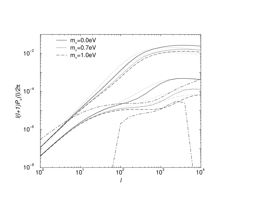
Fig. 1.: Weak Lensing Power Spectrum for two COBE normalized models involving non-zero mass neutrinos. The upper set of curves correspond to a flat cosmological model involving $\Omega_{m}=0.75$, $\Omega_{b}=0.05$, $h=0.65$, $n_{s}=1$, while the lower set of curves are for $\Omega_{m}=0.35$ with other parameters as above. In grey, we show weak lensing power spectra using Peacock & Dodds (1996) fitting function for nonlinear evolution of the power spectrum, calculated assuming its validity for MDM cosmologies, while dark lines show weak lensing power spectra for recently updated fitting functions for MDM cosmologies by Ma (1998). In dot-dashed lines, we show expected errors in the power spectrum measurement from a weak lensing survey of 25 $\times$ 25 deg² down to the magnitude limits of 25 in R. Such a survey is expected to be available in near future with wide-field cameras such as MEGACAM (Boulade et al. 1998).

In Fig.1, we show two sets of COBE normalized weak lensing power spectra considering the presence of non-zero mass neutrinos. The upper and lower curves represent two cosmological models with high and low $\Omega_{m}$ values and computed assuming the redshift of background sources as given in Eq.4, with $\beta=1.5$ and $\alpha=2.0$. As shown, non-zero mass neutrinos suppress power at large $l$ values, and this effect is significant for low $\Omega_{m}$ models. This is primarily due to that fact that the suppression of power is directly proportional to the ratio of $\Omega_{\nu}/\Omega_{m}$. In addition, we have also shown the expected 1$\sigma$ uncertainty in the power spectrum measurement for a survey of size 625 deg² down to magnitude limit of 25 in R. It is likely that weak lensing surveys down to R of 25 within an area of 100 deg² will be available in the near future, and that the area coverage would steadily grow as high as several thousand square degrees over the next decade. As shown in Fig.1, reliable measurements of the power spectrum is likely when $l$ is between 100 and 3000. This is the same range in which neutrinos suppress power. Such effects do not exist, for example, in the CMB anisotropy power spectrum; low redshift probes of the matter power spectrum provide ideal ways to weigh neutrinos.

2.3 Cosmic Confusion?

However, there are alternative possibilities which can mimic neutrinos. In Fig.2, as examples, we illustrate two possibilities which can produce a similar power spectrum as a model involving $\Omega_{m}$ of 0.35 and $m_{\nu}$ of 0.7 eV; When $m_{\nu}$ is 1 eV, increasing the primordial scalar tilt by 30% can mimic the original power spectrum, while in a model with zero mass neutrinos, increasing the baryon content by 80% can produce essentially the original power spectrum. Such effects are essentially what can be described as cosmic confusion, and thus, careful measurements of cosmological parameters are needed to weigh neutrinos even with weak lensing.

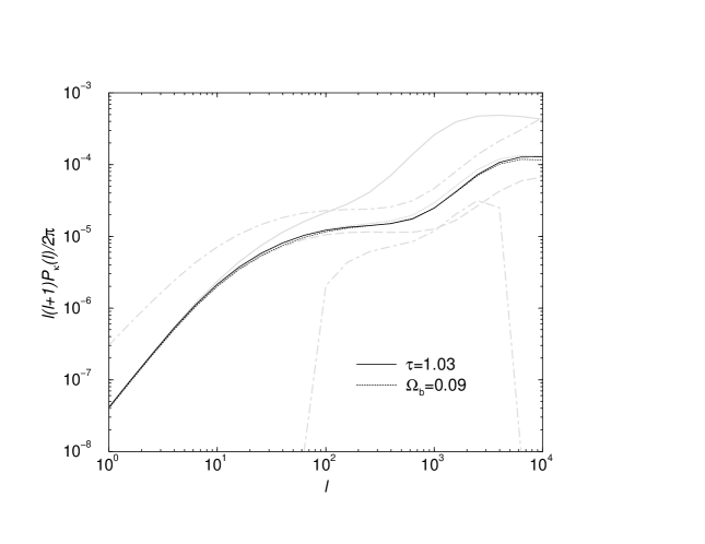
Fig. 2.: Cosmic confusion: Two alternate models involving changes in the baryon content or the scalar tilt produce essentially the same power spectrum as a model involving 0.7 eV neutrinos. The grey curves are same as Fig.1.

3 Neutrino Mass Measurement

In order to investigate the possibility for a neutrino mass measurement, we consider the so-called Fisher information matrix (e.g., Tegmark et al. 1997) with six cosmological parameters that define the weak lensing power spectrum. The Fisher matrix $F$ can be written as:

$$F_{ij}=-\left<\partial^{2}\ln L\over\partial p_{i}\partial p_{j}\right>_{\bf x},$$ (10)

where $L$ is the likelihood of observing data set ${\bf x}$ given the parameters $p_{1}\ldots p_{n}$. Following the Cramér-Rao inequality, no unbiased method can measure the ith parameter with standard deviation less than $(F_{ii})^{-1/2}$ if other parameters are known, and less than $[(F^{-1})_{ii}]^{1/2}$ if other parameters are estimated from the data as well. Since Eq.6 is usually calculated assuming a prior cosmological model, the estimated errors on the parameters of this underlying model can be dependent on prior assumptions.

Assuming a Gaussian and uncorrelated distribution for uncertainties, one can easily derive the Fisher matrix for weak lensing as:

$$F_{ij}=\sum_{l=l_{\rm min}}^{l_{\rm max}}\frac{f_{\rm sky}(2l+1)}{2\left(P_{\kappa}(l)+\frac{\langle\gamma^{2}\rangle}{n_{\rm mag}}\right)^{2}}\frac{\partial P_{\kappa}(l)}{\partial p_{i}}\frac{\partial P_{\kappa}(l)}{\partial p_{j}}.$$ (11)

As illustrated in Fig.2, in order to make a reliable measurement of neutrino mass, it is necessary that one consider external measurements of cosmological parameters. Such measurements can come from variety of probes such as Type Ia supernovae, galaxy clusters, CMB, gravitational lensing etc. Here, we take both a conservative approach with large uncertainties for the cosmological parameters based on other techniques and a more optimistic approach motivated by the expected uncertainties from future surveys. In our conservative model, we use following errors: $\sigma(\Omega_{m})=0.2$, $\sigma(\Omega_{b})=0.1\Omega_{b}$, $\sigma(h)=0.2$, $\sigma(n_{s})=0.1$, $\sigma(\ln\delta_{H})=0.5$, while in our optimistic model, we use $\sigma(\Omega_{m})=0.07$, $\sigma(\Omega_{b})=0.0025h^{-2}$, $\sigma(h)=0.1$, $\sigma(n_{s})=0.06$, $\sigma(\ln\delta_{H})=0.3$. These errors are in fact worser than what is expected to be measured from PLANCK, but is similar to what could be achieved with a mission such as MAP. We consider a fiducial model in which $\Omega_{b}=0.019$, consistent with current observations, $h=0.65$ and $n_{s}=1.0$ and normalization based on COBE. In addition, we also consider an alternative normalization to the power spectrum based on measurements of $\sigma_{8}$ ($=0.56\Omega_{m}^{-0.47}$) following Viana & Liddle (1998). We also consider variations to the above fudicial model and marginalize over the uncertainties to obtain the 2$\sigma$ detection limit of neutrinos for various weak lensing surveys. We only use the information on the power spectrum between $l$ values of 100 and 5000. At $l$ values below 100, cosmic variance dominate the measurement while at $l>5000$ the finite number of galaxies and their ellipticies contribute to the increase in power spectrum measurement uncertainties.

In Fig.3, we summarize our results: solid lines show the expected 2$\sigma$ detection limit for our conservative errors while dashed lines show the detection limits for more optimistic errors. The dot-dashed line is for models in which the matter power spectrum is normalized to 8 h^-1 Mpc scales. The high dependence of its value and error on $\Omega_{m}$ causes the $\sigma_{8}$ normalized limits to be different from those in which power spectra are normalized to COBE measurements. In Fig.3, we have shown the limits assuming a survey of 100 $\times$ 100 sqr. degrees down to a R band magnitude of 25. However, for surveys with different areas, especially for surveys in near future with small coverage, the limits can be scaled by the reduction factor in the observed area (see, Eq.12). We assume uncorrelated errors in the weak lensing power spectrum measurement. For low $\Omega_{m}$ models ($\mathrel{\mathchoice{\vbox{\offinterlineskip\halign{\hfil$\displaystyle#$\hfil\cr<\cr\sim\cr}}}{\vbox{\offinterlineskip\halign{\hfil$\textstyle#$\hfil\cr<\cr\sim\cr}}}{\vbox{\offinterlineskip\halign{\hfil$\scriptstyle#$\hfil\cr<\cr\sim\cr}}}{\vbox{\offinterlineskip\halign{\hfil$\scriptscriptstyle#$\hfil\cr<\cr\sim\cr}}}}0.5$) normalized to COBE, and using our conservative errors, we can write the 2 $\sigma$ detection limit on the neutrino mass as:

$$m_{\nu}^{2\sigma}\sim 5.5\left(\frac{\Omega_{m}h^{2}}{0.1N}\right)^{0.8}\left(\frac{10}{\theta_{s}}\right).$$ (12)

This 2 $\sigma$ detection limit is comparable to current upper limits at the 2 $\sigma$ level on the neutrino mass. Using more optimistic errors decreases this limit by a factor of 2 to 3 depending on $\Omega_{m}$, however, to obtain such optimistic errors on cosmological parameters one require accurate measurements on the CMB power spectrum such as to the level of MAP satellite. In making this prediction we have assumed that the weak lensing power spectrum can be measured to the expected uncertainty predicted by simple arguments involving errors in ellipticities and cosmic confusion and that the measurements are uncorrelated. Also, in order to obtain a reliable measurement of the weak lensing power spectrum, one require additional knowledge on the redshift distribution of sources. Such information is likely to be adequately obtained with photometric redshift measurements of color data or by template fitting techniques that has been developed for multicolor surveys (e.g., Hogg et al. 1998). The accuracy to which such measurements can be made should be adequate, however, if no multicolor data is available then this may not be possible. Therefore, it is likely that such a clean measurement of the weak lensing power spectrum will not be directly possible in the near future. In order to consider such affects, we increased the expected uncertainties in the power spectrum by a factor of 2 beyond what is predicted for a survey of 100 sqr. degrees down to a R band magnitude of 25. The expected neutrino mass limit increases by an amount consistent with what is expected from the Fisher matrix formalism. Even in such a scenario with a poorly measured power spectrum, one can still put interesting limits on the neutrino mass.

A small area survey such as 10 $\times$ 10 sqr. degrees is likely to be feasible in the near future with upcoming observations from wide field CCD cameras. There are several such instruments currently either in the design or manufacturing stages: MEGACAM which will make observations from the Canada France Hawaii Telescope (CFHT; Boulade et al. 1998), VLT-Survey-Telescope (VST). Other than these surveys, which are likely to first produce deep weak lensing surveys over small areas, two wide-field shallow surveys are currently ongoing at optical (SDSS; Stebbins et al. 1997) and radio (FIRST; Kamionkowski et al. 1997), however, it is still unclear as to what accuracy these imaging data can be used for weak lensing studies. Still, assuming that SDSS can in fact make weak lensing measurements down to a R band magnitude of 22, we find that given its wide field coverage, it can also be used to detect neutrinos down to a mass limit of $\sim$ 3 eV at the 2$\sigma$ level, or to put interesting limits at the same mass threshold. For an ultimate survey of $100\times 100$ deg², weak lensing allows a detection of neutrinos down to a mass of $\sim$ 0.5 eV when $\Omega_{m}\sim 0.3$ and $h\sim 0.65$. With expected errors from CMB satellites, this limit can be lowered by a factor of 3 to 4 allowing a possibility for weak lensing surveys to probe neutrinos with mass lower than 0.1 eV. These conclusions, generally, are consistent with what was found by Hu & Tegmark (1999); minor differences are likely to arise from the fact that the present study and Hu & Tegmark (1999) used different fitting functions to describe the non linear evolution of the potential power spectrum and that fudicial cosmological models may be different. We note here that using MAP or PLANCK data with galaxy redshift surveys such as from SDSS, and no weak lensing measurements, only allow the determination of neutrino mass to a limit of $\sim$ 1 eV and 0.3 eV respectively (Hu et al. 1997).

Fig. 3.: Expected 2$\sigma$ detection limit for 100 $\times$ 100 deg.² weak lensing survey down to a magnitude limit of 25, assuming a spatially flat Universe with a scalar tilt of 1. Solid line represents detection with our conservative errors while the dashed line represent detection with more optimistic errors. The dot-dashed line is for models involving normalizations based on current measurements of $\sigma_{8}$ and using more optimistic errors.

Returning to much smaller surveys, we have only studied the accuracy to which the neutrino mass can be measured. However, in making such measurements one does not lose information to make other measurements as well. For example, the conservative errors we assumed on other cosmological parameters can also be improved by factors of 2 to 3 when information on these parameters are also derived with weak lensing. Also, one can abandon the assumption of a spatially flat Universe, and determine the value of the cosmological constant directly from weak lensing data, while also putting a limit on the neutrino mass. However, if the assumption on a spatially flat Universe is dropped in order to measure $\Omega_{\Lambda}$, then the limit to which neutrino mass can be measured increases by a factor of $\sim$ 1.5 for surveys of size 100 sqr. degrees. For now, if one to measure or improve all other cosmological parameters that can be studied with weak lensing surveys (and listed in Sect.2.1), then it is safe to say that neutrinos down to a mass limit of $\sim$ 8 eV can be measured with weak lensing surveys of size 100 sqr. degrees down to a R band magnitude of 25. Such a possibility will definitely be available with upcoming surveys from MEGACAM. For still smaller surveys, such as 10 sqr. degrees, if one attempts to make all cosmological measurements, such as $\Omega_{m}$ and $\Omega_{\Lambda}$ interesting limits on neutrino mass can only be obtained at a mass level greater than 25 eV. Since such neutrino masses may be ruled out, it is safe to ignore the presence of neutrinos when making measurements with much smaller surveys. Such surveys are likely to be first available with wide-field cameras, with the coverage increasing afterwards.

4 Discussion & Summary

Here, we have considered the possibility for a neutrino mass measurement using weak gravitational lensing of background sources due to foreground large scale structure. For survey of size 100 deg², neutrinos with masses greater than $\sim$ 5.5 eV could easily be detected. This detection limit is comparable to the current cosmological limits on neutrino mass, such as from the Ly$\alpha$ forest. When compared to various ongoing experiments to detect neutrinos, the advantage of weak lensing is that one can directly obtain a measure of mass rather than mass difference between two neutrino species. For typical surveys of size $\sim$ ten square degrees, ignoring the presence of neutrinos can lead to biased estimates for cosmological parameters, e.g., cosmological mass density can be underestimated by a factor as high as $\sim$ 15% if neutrinos with mass 5 eV are in fact present. However, if such weak lensing surveys are solely used for the derivation of parameters such as cosmological mass density, than the accuracy to which such derivations can be made is less than the bias produced by neutrinos. Therefore, for small area surveys, the presence of neutrinos can be safely ignored (assuming that their masses is less than $\sim$ 5 eV or so). However, armed with cosmological parameters from other complimentary techniques, even such small weak lensing surveys allow a strong possibility to investigate the presence of non-zero mass neutrinos.

We acknowledge useful discussions with Wayne Hu and Dragan Huterer. Wayne Hu is also thanked for communicating the fitting code to evaluate the MDM transfer function. We also thank an anonymous referee for comments which led to several improvements in the presentation.

References

- 1 Bartelmann M., Schneider P. 1999, A&A in press (astro-ph/9902152).
- 2 Beacom J. F. 1999, in 22nd Symposium on Nuclear Physics (astro-ph/9901300).
- 3 Beacom J. F., Vogel P. 1998, PRD 58, 093012.
- 4 Bernardeau F., Waerbeke L. V., Mellier Y. 1997, A&A 322, 1.
- 5 Boulade O., Vigroux L., Charlot X., et al., 1998, MEGACAM, the next Generation Wide-Field camera for CFHT. SPIE vol. 3355, Astronomical Telescopes and Instrumentation, Kona Hawaii, March 1998.
- 6 Blandford R. D., et al. 1991, MNRAS 251, 60.
- 7 Bunn E., White M. 1997, ApJ 480, 6.
- 8 Carroll S.M., Press W.H., Turner E.L. 1992, ARAA 30, 499
- 9 Cooray A. R., Quashnock J. M., Miller M. C. 1998, ApJ 511, 562.
- 10 Croft R. A. C., Hu W., Dave R., PRD submitted, astro-ph/9903335.
- 11 Eisenstein D. J., Hu W., 1999, ApJ 511, 5.
- 12 Fogli G. L., Lisi E., Montanino D., Scioscia G. 1997, PRD 56, 4365.
- 13 Fukuda Y., et al. 1998, PRL 81, 1562.
- 14 Hogg D. W., Cohen J. G., Blandford R., et al. 1998, AJ 115, 1418.
- 15 Hu W., Tegmark M. 1999, ApJ 514, L65.
- 16 Hu W., Eisenstein D. J. 1998, ApJ 498, 497.
- 17 Hu W., Eisenstein D., Tegmark N. 1997, astro-ph/9712057.
- 18 Jain B., Seljak U. 1997, ApJ 484, 560.
- 19 Kaiser N. 1998, ApJ 498, 26.
- 20 Kamionkowski M., Babul A., Cress C. M., Refregier A., 1999, MNRAS 301, 1064.
- 21 Lineweaver C., 1998, ApJ 505, L69
- 22 Ma C.-P., 1998, ApJ 508, L5.
- 23 Ma C.-P., 1999, preprint (astro-ph/9904001).
- 24 Mellier Y., 1998, ARA&A (in press), astro-ph/9812172.
- 25 Miralda-Escude J. 1991, ApJ 380, 1.
- 26 Peacock J. A., Dodds S. J. 1996, MNRAS 267, 1020
- 27 Perlmutter S., Aldering G., Valle M. D., et al. 1998, Nat 391, 51
- 28 Riess A. G., Fillippenko A. V., Challis P., et al., 1998, AJ 116, 1009
- 29 Schneider P., et al. 1998, MNRAS 296, 873.
- 30 Shi X., Fuller G. M. 1999, PRD D59, 063003.
- 31 Smail I., et al. 1995, ApJ 449, L105.
- 32 Smith C., Klypin A., Gross M., Primack J. R., Holtzman J. 1998, MNRAS 297, 910.
- 33 Stebbins A., McKay T., Frieman J. A. 1995, astro-ph/9510012.
- 34 Tegmark M., Eisenstein, D., Hu, W., Kron, R., 1998, preprint (astro-ph/9805117).
- 35 Tegmark M., Taylor A. N., Heavens A. F., 1997, ApJ 480, 22.
- 36 Totani T. 1998, PRL 80, 2039.
- 37 van Waerbeke L., Bernardeau F., & Mellier Y., 1999, A&A 342, 15.
- 38 Vianna P. T. P., Liddle A. R. 1996, MNRAS 281, 323.
- 39 White M., 1998, ApJ 506, 495