The interstellar clouds of Adams and Blaauw revisited: an HI absorption study - I

Abstract

This investigation is aimed at clarifying the nature of the interstellar gas seen in absorption against bright O and B stars. Towards this end we have obtained for the first time HI absorption spectra towards radio sources very close to the lines of sight towards 25 bright stars previously studied. In this paper we describe the selection criteria, the details regarding our observations, and finally present the absorption spectra. In the accompanying paper we analyse the results and draw conclusions.

1 Introduction

We have carried out an absorption study in the 21 cm line of atomic hydrogen in 25 directions in the Galaxy. These directions have been selected from previous optical absorption studies in the lines of singly ionized calcium (CaII) and neutral sodium (NaI). In this paper, we describe the observations and present the data obtained by us. A discussion of the results and the conclusions drawn from the study are in the accompanying paper (Rajagopal, Srinivasan and Dwarakanath 1998; paper II).

Our observations were primarily intended to study the velocities of the HI absorption features, their linewidths, and in combination with existing HI emission measurements obtain the spin temperature of the absorbing gas. Our study was motivated by the following questions:

• How are interstellar clouds seen in optical absorption related to those seen in HI absorption and emission ?

• What is the nature of the relatively fast clouds so commonly seen in the absorption lines of NaI and CaII ?

To clarify these and related issues we briefly summarize the salient historical background. Some of the earliest information about the Interstellar Medium (ISM) came from observations of optical absorption in the H and K ($\lambda\lambda 3933,3968{\rm\AA}$) lines of CaII, and the D₁ and D₂ ($\lambda\lambda 5889,5895{\rm\AA}$) lines of NaI towards bright stars. Adams (1949) made an extensive study of the absorption lines of CaII towards nearly 300 O and B stars. These observations were later extended to the D lines of NaI (Routly and Spitzer 1952; Hobbs 1969), and to high latitude stars (Münch and Zirrin 1961).In the simplest model, these lines were attributed to interstellar gas in the form of clouds. The existence of a hot intercloud medium was conjectured by Spitzer (1956) and the theoretical basis for a two-phase model followed ( Field 1965; Field, Goldsmith and Habing 1969).

Independently, a global picture of the ISM emerged from radio observations of the 21 cm HI line (Clark, Radhakrishnan and Wilson 1962; Clark 1965; Radhakrishnan et. al. 1972). These and later studies have established that an important constituent of the ISM are cool diffuse clouds in pressure equilibrium with a warmer intercloud medium. The notion of interstellar “clouds” was thus invoked to explain both optical and radio observations. But one was left speculating as to whether the two populations were the same. Surprisingly the answer to the above question still remains incomplete. Many properties of the two populations seem to differ. In particular the number of clouds per kiloparsec (Blaauw 1952; Radhakrishnan and Goss 1972; Hobbs 1974; Radhakrishnan and Srinivasan 1980), and the velocity distributions deduced from optical and radio observations, respectively, do not agree. The latter discrepancy is discussed in more detail in a subsequent section.

In this study, we have attempted a direct comparison by doing HI absorption measurements towards the bright stars themselves. Of course, this can be done only in those lines of sight (towards stars studied previously) where there are strong enough radio sources. We were actually able to do this in about 25 directions. From this data we obtain the velocities of the absorbing gas, and in combination with previous emission measurements in the same directions, the spin temperature of the HI gas in the very entities seen in optical absorption. This is the first attempt at such a direct comparison.

Identifying the optical absorption lines with 21 cm absorption features is particularly important because of a long standing puzzle. Optical absorption along many lines of sight reveal two sets of absorption features. One set occur at near zero (low) velocities and another at higher velocities with respect to the local standard of rest. The faster clouds have measured velocities well in excess of the radial component of Galactic rotation one could attribute to them. In a classic study of Adams’ data, Blaauw (1952) clearly showed the existence of a high velocity tail extending upto as high as 100 km s^-1in the distribution of random velocities of the optical absorption features. Thus the existence of a high velocity population of clouds was firmly established. There was also a hint that these “fast” clouds may belong to a different population. They exhibited the well known Routly-Spitzer effect (Routly and Spitzer 1952) i.e., the NaI to CaII ratios in these clouds were significantly lower than those in the lower velocity clouds.

In the decade following the discovery of the 21 cm line attempts were made to detect the gas seen in optical absorption. These involved measuring HI emission in the direction of stars which show optical absorption features in their spectra in order to compare the HI spectra with the CaII and NaI spectra (Takakubo 1967; Habing 1968, 1969; Goldstein and MacDonald 1969; Goniadzki 1972; Heiles 1974 and others). Habing’s study in particular targeted selected stars to attempt a direct face off. The results of these early studies threw up another intriguing fact. The low velocity features appeared to be well correlated in HI emission and optical absorption, i.e., whenever the optical spectra showed a low velocity absorption feature (v$<$ 10 km s^-1), there was HI emission at the corresponding velocity. However, the high velocity features were in general absent in HI emission down to low limits (T${}_{b}<$ 1 K). This seemed to be the case in all directions in the sky.

The typical beam sizes in the early experiments to measure HI emission were $\sim$ 0.5^∘. The angular size of the absorbing gas could have been much smaller leading to considerable beam dilution. This could be the reason why the clouds were not detected in HI emission. This exemplifies the difficulties in comparing the features seen in optical absorption with arc-second resolution with those seen in radio emission using a comparatively large beam. This is one of the major factors which led us to attempt an HI absorption study. The resolution achieved is of the same order as in optical absorption enabling a surer comparison.

Despite the failure of the early emission measurements to detect the “fast” clouds there is some indication for a population of high velocity clouds from an independent HI absorption study, though this is far from being firmly established. Radhakrishnan and Srinivasan (1980) from a detailed analysis of the 21 cm absorption profile towards the Galactic centre suggested that the peculiar velocities of HI clouds cannot be understood in terms of a single Gaussian distribution with a dispersion of about 5 $-$ 7 km s^-1, the velocity distribution for “standard” HI clouds. There was an indication of a second population of weakly absorbing clouds with a velocity dispersion $\sim 35$ km s^-1. But this has not been confirmed by other studies. Our study is an attempt to address this important but neglected problem.

2 Scope of the present observations

We chose 25 stars towards which both low and high velocity absorption features have been seen (from CaII or NaI atoms or both). Two of the stars HD 14134 and 14143 happen to be in the same field (in our radio observations) and hence we have measured absorption in only 24 fields. The positions of all the selected stars as projected on the plane of the Galaxy are shown in Fig 1. The Galactic spiral arms shown in this

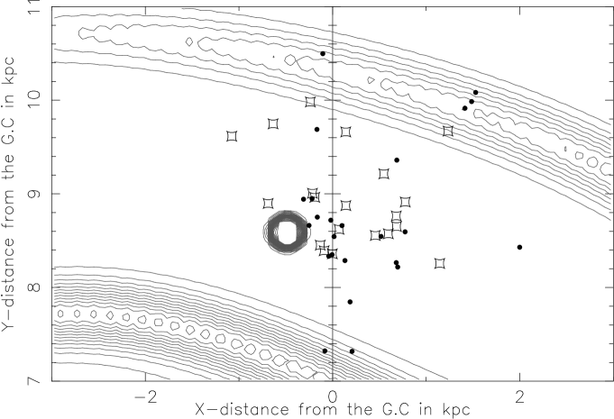
Figure 1: 24 of our sample of 25 stars (HD 119608 lies outside the region shown) are shown as dots on the contour plot of the Galactic spiral arms from Taylor and Cordes. The squares show the local OB associations from Blaauw (1985). The Sun is at 8.5 kpc from the Galactic center. The object with dense contours to the left of the sun is the Gum Nebula. The outer arm shown is the Perseus arm, while the inner one is the Sagittarius arm. The three stars bunched together well inside the Perseus arm are HD 14134, 14143 and 14818. The Perseus OB1 cluster is seen close to them. The two stars seen projected on the Sagittarius arm are HD 166937 and 159176. These fields show high velocity HI absorption.

figure are from the electron density model by Taylor and Cordes (1993). In 13 of these directions HI emission measurements had been carried out earlier by Habing (1968,1969). Most of the fields studied by Habing were chosen at $|\rm b|$ $>$ 20 ^∘ to avoid complicated HI emission arising in the plane. Four stars, however, have $|\rm b|$ $<$ 10^∘ and were selected since they show CaII velocities well outside the limits of Galactic rotation at the estimated distances. Out of the remaining 12 fields, 3 have been investigated by Goniadzki (1972) for HI emission and one by Takakubo (1967). The rest of the fields have not been investigated in the radio. However, we have been able to get the brightness temperatures and column densities of HI in these directions also from the Leiden-Green Bank survey (Burton 1985).

In the observations described in this paper we have obtained HI absorption spectra towards a radio source whose line of sight is close to that of the star in each of the 24 fields. We have been able to identify fairly strong radio sources (in most cases $\stackrel{{\scriptstyle>}}{{{}_{\sim}}}\,$ 50 mJy at 21 cm) within 30’ to 40’ of the star in every field. In more than half the fields the radio sources are within 10’ and several within 5’ of the star in question. If the cloud is halfway to the star, then given a 10’ separation between the star and the radio source one will sample a cloud of size less than 2 pc even for the farthest stars in the sample which are about 2 kpc away. This is well within the range of accepted sizes for standard clouds (Spitzer 1978). In some fields we had to arrive at a compromise between the minimum cloud size we could sample (i.e., the proximity of the projected position of the background source to the star) and the optical depth sensitivity we could achieve. The latter constrains us to fairly strong radio sources for reasonable integration times. This flux density requirement limits the number of sources that one can find close to the star and hence the trade off. Most of the background sources selected are from the NRAO/VLA Sky Survey (Condon et al. 1996). We aimed at an optical depth sensitivity of $\tau$ = 0.1 and have done better than that in several cases. The worst case limit on the optical depth is 0.4.

3 Observations and data analysis

We obtained the absorption spectra using the Very Large Array (VLA) in the $\sim$ 1 km and $\sim$ 11 km configurations with a synthesized beam size of 44” and 4”, respectively, at 21 cm. The observations were carried out with a total bandwidth of 1.56 MHz using both polarizations and 128 channels. We used 0134+329 as the primary flux calibrator. For each source we observed a nearby secondary calibrator to do a phase and bandpass calibration. The calibrator was observed with the frequency band shifted by 1.5 MHz, corresponding to a velocity shift $\sim$ 300 km s^-1. This shift in velocity is sufficient to move the band away from any Galactic feature which might affect the bandpass calibration. Typically, each of these calibrators were observed for $\sim$ 10 minutes. The typical strengths of these calibrator sources being $>$ 1 Jy, 10 minutes of integration time was sufficient to achieve a signal-to-noise ratio greater than that on the source by a factor of 2. After on line Hanning smoothing over 2 channels, the frequency resolution obtained was $\sim$ 12 kHz which corresponds to a velocity resolution of $\sim$ 2.5 km s^-1. The integration time on each source was chosen to give an optical depth sensitivity of $\tau\sim$ 0.1, and ranged from a few minutes to more than an hour. In all a total of $\sim$ 30 hours were spent on the sources, split over several sessions of observing.

The analysis was carried out using the Astronomical Image Processing System (AIPS) developed by the National Radio Astronomy Observatory (NRAO). The first step was to make continuum images of each field and examine them for bright sources, including the target source. Our observations coincided with the ongoing NRAO/VLA Sky Survey (in the B and D configurations) and most of our observations were carried out during the daytime. Hence we had to contend with moderate to strong levels of interference over most of the band owing to which approximately 10% of the data was lost. The next stage involved removing the continuum level from all channels. The task used for this was UVLIN. The continuum level to be removed is determined from a linear fit to the visibility levels in selected channels, which are chosen to be free of interference as well as any spectral features. Finally the image cubes were made. The imaging was typically done over an area of 512 by 512 pixels. In some cases several cubes were synthesised for different areas to cover all the sources of interest in the field. The spectra towards each of the sources were analysed with the Groningen Image Processing System (GIPSY; van der Hulst et al. 1992).

Field	d	lII, bII	$\theta$	Vlsr	$\tau$	VGal
	pc		arcmin	km s-1		km s-1
14143∗	2000	135, $-$4	10.0	$-$52.8, $-$50.3, $-$46.1,	0.09	$-$25
				$-$11.2, $-$8.2
14818	2200	136, $-$4	10.0	$-$55.8, $-$14.0, $-$3.7	0.05	$-$25
21278	190	148, $-$6	37.0	2.8	0.08	$>$0
21291	1100	141, 3	36.0	$-$31.2, $-$7.0, $-$4.9	0.07	$-$10
24912	46	160, $-$13	2.2	4.3, 6.0, $-$82.0	0.39	$-$5
25558	220	185, $-$33	26.0	8.1	0.10	$<$0
34816	540	215, $-$26	40.0	6.0, 8.0	0.10	$<$0
37742	500	206, $-$16	15.0	9.5	0.03	5
38666	300	237, $-$27	21.5	none	0.02	5
41335	300	213, $-$13	3.0	1.0, 10.0	0.04	$>$0
42087	1200	188, 2	42.0, 32.0	4.4, 6.5, 12.4	0.13	$-$5
93521	2000	183, 62	27.0	none	0.11	$<$0
119608	3400	320, 43	16.0	$-$5.4	0.09	$-$20
141637	170	346, 21	11.0	0.5, $-$0.2	0.28	$\sim$0
148184	150	358, 21	0.82	3.4	0.26	$\sim$0
156110	720	71, 36	$<$10.0	2.2	0.18	5
159176	1180	356, 0	5.3	$-$20.8, $-$74.0	0.28	$\sim$0
166937	1200	10, $-$2	5.0, 7.0	34.6, 47.2, 35.7	0.39	5
175754	680	16, $-$10	$<$10.0	6.8	0.09	10
199478	2000	88, 1	8.0	5.0 to $-$75.0	0.21	$-$7
205637	250	32, $-$45	18.4	none	0.30	5
212978	520	95, $-$15	12.0	0.3, $-$12.3	0.04	$-$5
214680	780	97, $-$17	12.0	$-$4.8, 1.4	0.28	$-$5
220172	750	68, $-$63	2.9	none	0.33	10

Table 1: Summary of HI absorption: Column 1 gives the HD number of the star. Columns 2 and 3 show the distance to the star (as listed in the Sky Catalogue 2000.0, Vol 1, Hirshfield and Sinnott 1982) and its galactic coordinates, respectively. Column 4 gives the angular separation of the star from the radio source(s) towards which absorption has been detected. Column 5 lists the HI absorption velocities (LSR). Columns 6 shows the detection limit in $\tau$ (towards the strongest source in the field). Column 7 shows the approximate radial component of the Galactic rotation velocity at the distance to the star. $<$ 0 and $>$ 0 are used to indicate velocities with magnitude less than 5 km s^-1.
The stars 14134 and 14143 are in the same field referred to above as 14143^∗.

Field	Vlsr(optical, all)	Vlsr(HI, coincident)	VGal	Ref
	km s-1	km s-1	km s-1
14143∗	$-$62.3, $-$46.8, $-$6.3	$-$46.1, $-$50.3, $-$11.2	$-$25	M
	$-$65.3, $-$50.8, $-$10.3
14818	$-$42.6, $-$33.6, $-$6.6	$-$3.7	$-$25	M
21278	$-$0.2, 48.6	2.8	$>$0	A
21291	$-$34.0, $-$7.5	$-$31.2, $-$7.0, $-$4.9	$-$10	M
24912	4.7, 20.7	4.3	$-$5	A
25558	10.1, 19.0	8.1	$<$0	A
34816	$-$14.0, 4.14	6.0	$<$0	A
37742	$-$21.0, 3.6	none	5	A
38666	1.0, 20.2	no absorption	5	MZ
41335	$-$20.8, 0.2	1.0	$>$0	A
42087	$-$37.7, $-$4.8, 10.2	12.4	$-$5	A
93521	$-$55.0, $-$34.0, $-$10.3, 6.8	no absorption	$<$ 0	MZ
119608	1.3, 22.4	none	$-$20	MZ
141637	$-$22.0, 0.0	0.5, $-$0.2	0	B
148184	14.2, 2.2	3.4	0	A
156110	$-$19.7, 0.4	2.2	5	MZ
159176	3.5, $-$22.5	$-$20.8	0	A
166937	$-$5.5, 5.9, 25.3, 41.1	5.4, 47.2, 35.7	5	A
175754	$-$73.0, 5.9, 29.5	6.8	10	A
199478	$-$2.1, 8.7, 42.3, 61.2	3.8 (blend)	$-$7	A
205637	$-$13.9, 1.8	no absorption	5	A
212978	$-$73.0, 0.6	0.3	$-$5	A
214680	$-$23.7, $-$14.7, 0.1	1.4	$-$5	A
220172	$-$21.5, $-$0.8, 13.5	no absorption	10	MZ

Table 2: Summary of coincident velocities: Column 2 lists the LSR velocities of all the optical absorption features seen in each line of sight (most of the listed velocities are from CaII observations). Velocities of the matching HI absorption features are given in column 3. Column 4 shows the radial component of the Galactic rotation velocity at the distance to the star. Column 5 has the reference for the optical absorption velocities which are from A: Adams (1949), B: Buscombe and Kennedy (1962), M: Münch (1957) and MZ: Münch and Zirrin (1961).

4 Results

Table 1 lists the details of all the fields observed. In most of these fields there were several radio sources within the primary beam in addition to the source initially targeted. We have obtained spectra towards these sources as well if they turned out to be strong enough to detect reasonable optical depths ($\sim$ 0.1). Column 1 gives the HD number of the star. Columns 2 and 3 give the distance to the star (as listed in the SKY 2000 catalogue of bright stars) and its galactic coordinates, respectively. Column 4 gives the angular separation of the star from the radio source(s) towards which absorption has been detected. Column 5 lists the HI absorption velocities (LSR).These velocities have been derived by fitting Gaussian profiles to the absorption features. Columns 6 shows the detection limit in $\tau$ (towards the strongest source in the field). Column 7 shows the radial component of the Galactic rotation velocity at the distance to the star.

The optical absorption velocities are likely to suffer from blending of features due to lack of resolution. A discussion of this and associated problems can be found in Welty, Morton and Hobbs (1996). Moreover, the correction for the solar motion adopted by different authors may differ leading to errors of $\sim$ 1 km s^-1(see for example Blaauw, 1952). In some cases, we have smoothed the absorption spectra to a resolution of 5 km s^-1to facilitate the convergence of the gaussian fit. Narrow absorption features are known to have widths less than this (Crovisier 1981). We have checked the unsmoothed data to ensure that there are no serious effects of blending in the estimates for velocities for the features discussed below. However, crowding in velocities inevitably causes some of the absorption widths to be suspect. The formal error in the fitting procedure for our HI absorption velocities is in most cases $\sim$ 1 km s^-1or less. The errors add to $\stackrel{{\scriptstyle<}}{{{}_{\sim}}}\,$2 km s^-1. However, it must be stated that the blending of features in both optical and radio could easily lead to larger errors than this formal value. Hence we consider a feature in the optical spectrum as “coincident” with one seen in HI absorption or emission if the magnitude of the difference in velocities is less than 3 km s^-1. This is roughly the same criterion adopted by Habing (1969) and Howard et al. (1963) for comparing HI emission profiles with optical absorption.

Table 2 lists the “matching” features i.e., HI absorption features whose velocities agree with the velocity of the optical absorption feature. Column 2 shows the LSR velocities of all the optical absorption features seen in each line of sight (most of the listed velocities are from CaII observations). Velocities of the matching HI absorption features follow in column 3. Column 4 shows the radial component of the Galactic rotation velocity at the distance to the star to facilitate comparison with the optical absorption velocities. Column 5 has the reference for the optical absorption velocities which are from Adams (1949), Münch (1957) and Münch and Zirrin (1961). We have used later compilations of these by Takakubo (1967), Siluk and Silk (1974), and Habing (1969).

We present the HI optical depth towards all the observed fields at the end of the paper. The coordinates of the radio source (epoch 1950) towards which the spectrum is obtained is labelled at the top right of each panel. The HD number of the star towards which the corresponding optical spectrum is obtained is at the top left. The star co-ordinates (epoch 1950) are given immediately below this. The star co-ordinates have not been repeated if there are several radio sources in the same field. In all the spectra the velocities at which optical absorption is seen is indicated by arrows on the velocity axis (top). The conclusions we draw from these observations and a detailed discussion of the implications for the models of the ISM are presented in paper II.

HI optical depth $\tau$ versus V_LSR. The arrows indicate the velocities of the optical absorption lines towards the star indicated above each panel.

References

- [1] Adams, W.A. 1949, Astrophys. J., 109, 354. 131.
- [2] Blaauw, A. 1952, B.A.N., 11, 459.
- [3] Blaauw, A. 1985, in IAU Symp. 106, The Milky Way Galaxy, eds. H.van Woerden, R.J.Allen and W.B.Burton, p.335.
- [4] Burton, W.B. 1985, Astr. Astrophys. Supp., 62, 365.
- [5] Buscombe, W., Kennedy, P.M. 1962, Mon. Not. R. astr. Soc., 125, 195.
- [6] Clark, B.G. 1965, Astrophys. J., 142, 1398.
- [7] Clark, B.G., Radhakrishnan, V., and Wilson, R.W. 1962, Astrophys. J., 135, 151.
- [8] Condon, J.J., Cotton, W.D., Greisen, W.E., Yin, Q.F., Perley, R.A., Taylor, G.B., Broderick, J.J 1996, Astr. J., 115, 1693.
- [9] Crovisier. J. 1981, Astr. Astrophys., 94, 162.
- [10] Field, G.B. 1965, Astrophys. J., 142, 531.
- [11] Field, G.B., Goldsmith, D.W., Habing, H.J. 1969, Astrophys. J.(Letters), 155, L149.
- [12] Goniadzki, D. 1972, Astr. Astrophys., 17, 378.
- [13] Goldstein, S.J., MacDonald, D.D. 1969, Astrophys. J., 157, 1101.
- [14] Habing, H.J. 1968, B.A.N., 20, 120.
- [15] Habing, H.J. 1969, B.A.N., 20, 171.
- [16] Heiles, C. 1974, Astrophys. J.(Letters), 193, L31.
- [17] Hirshfeld, A. and Sinnott, R.W. 1982 (eds), Sky Catalogue 2000.0, Vol 1, Sky Pub. Corp. and Cambridge Univ. Press.
- [18] Hobbs, L.M. 1969, Astrophys. J., 157, 135.
- [19] Hobbs, L.M. 1974, Astrophys. J., 191, 395.
- [20] Howard III, W.E., Wentzel, D.G., McGee, R.X. 1963, Astrophys. J., 138, 988.
- [21] Münch, G. 1957, Astrophys. J., 125, 42.
- [22] Münch, G., and Zirrin, H. 1961, Astrophys. J., 133, 11.
- [23] Radhakrishnan, V., Goss, W.M. 1972, Astrophys. J. Suppl., 24, 161.
- [24] Radhakrishnan, V., Goss, W.M., Murray, J.D., Brooks, J.W. 1972, Astrophys. J. Suppl., 24, 49.
- [25] Radhakrishnan, V. and Srinivasan, G. 1980, J. Astrophys. Astr., 1, 47.
- [26] Rajagopal, J., Srinivasan, G., and Dwarakanath, K.S. (paper II) 1998, J. Astrophys. Astr., submitted.
- [27] Routly, P.M., and Spitzer, L.Jr. 1952, Astrophys. J., 115, 227.
- [28] Siluk, R.S., and Silk, J. 1974, Astrophys. J., 192, 51.
- [29] Spitzer, L.Jr. 1956, Astrophys. J., 124, 20.
- [30] Spitzer, L.Jr. 1978, Physical Processes in the Interstellar Medium (New York:Wiley-Interscience).
- [31] Takakubo, K. 1967, B.A.N., 19, 125.
- [32] Taylor, J.H., Cordes, J.M. 1993, Astrophys. J., 411, 674.
- [33] van der Hulst, J.M., Terlouw, J.P., Begeman, K., Zwitzer, W., Roelfsema, P.R., in GIPSY in Astronomical Data Analysis Software and Systems I, eds. D.M.Worall, C.Biemesderfer,
- [34] Welty, D.E., Morton, D.C., Hobbs, L.M. 1996, Astrophys. J. Suppl., 106, 533.