Prediction of the In-Situ Dust Measurements of the Stardust Mission to Comet 81P/Wild 2

Abstract

We predict the amount of cometary, interplanetary, and interstellar cosmic dust that is to be measured by the Cometary and Interstellar Dust Analyzer (CIDA) and the aerogel collector on-board the Stardust spacecraft during its fly-by of comet P/Wild 2 and during the interplanetary cruise phase. We give the dust flux on the spacecraft during the encounter with the comet using both, a radially symmetric and an axially symmetric coma model. At closest approach, we predict a total dust flux of $10^{6.0}\;{\rm m}^{-2}\;{\rm s}^{-1}$ for the radially symmetric case and $10^{6.5}\;{\rm m}^{-2}\;{\rm s}^{-1}$ for the axially symmetric case. This prediction is based on an observation of the comet at a heliocentric distance of $1.7\;{\rm AU}$. We reproduce the measurements of the Giotto and VEGA missions to comet P/Halley using the same model as for the Stardust predictions. The planned measurements of interstellar dust by Stardust have been triggered by the discovery of interstellar dust impacts in the data collected by the Ulysses and Galileo dust detector. Using the Ulysses and Galileo measurements we predict that $25$ interstellar particles, mainly with masses of about $10^{-12}\ {\rm g}$, will hit the target of the CIDA experiment. The interstellar side of the aerogel collector will contain $120$ interstellar particles, $40$ of which with sizes greater than $1\ {\rm\mu m}$. We furthermore investigate the “contamination” of the CIDA and collector measurements by interplanetary particles during the cruise phase.

1 Introduction

The Stardust mission to comet 81P/Wild 2 is dedicated to the in situ measurement and sample return of cosmic dust. At the comet the pristine cometary material is investigated which is assumed to be a good sample of the nebula from which the Solar System has formed. Pre-solar interstellar grains that survived the formation process may therefore be present in the samples collected or measured in situ. On the way to the comet the opportunity is taken to investigate contemporary interstellar dust that traverses the Solar System and originates from the local interstellar low-density diffuse cloud which crosses the Sun’s way through the Milky Way [17]. We predict the dust flux on the two main instruments on-board Stardust, the aerogel dust collector and the Cosmic and Interstellar Dust Analyzer (CIDA) [7]. The dust collector is a plate with an area of $\approx 0.1\;{\rm m}^{2}$ that is to be exposed to the dust stream. Particles hitting the collector are trapped inside the aerogel [2]. CIDA is an in-situ impact plasma dust detector with a time-of-flight mass spectrometer similar to the PUMA/PIA instruments flown on Giotto [28]. Stardust launches in February 1999 and flies by Earth in January 2001 for gravity assist. The slow ($6.1\ {\rm km}\ {\rm s}^{-1}$) fly-by of comet P/Wild 2 occurs on January 1st, 2004 at a heliocentric distance of $1.86\ {\rm AU}$ when the comet is on the out-bound part of its orbit. During the fly-by the distance of the spacecraft to the comet nucleus is $\approx 100\ {\rm km}$, and the phase angle, i.e. the Sun–comet–spacecraft angle, is $70^{\circ}$. After fly-by Stardust returns to Earth in January 2006, where the sample-return capsule that contains the aerogel collector is separated from the spacecraft and sent to a direct entry into Earth’s atmosphere. The collection and in situ measurement of interstellar dust occurs during the cruise phase as shown in figure 1.

Figure 1: The trajectory of Stardust (solid line) in the ecliptic plane (the verenal equinox direction is to the right). The orbits of P/Wild 2 and Earth are indicated as dashed lines. Mission events are marked with the time given in days after launch in brackets. The flow direction of interstellar particles from the LIC as derived from the Ulysses/ Galileo measurements is shown by the arrow in the lower left corner. Thick lines indicate the part of the orbit used to collect interstellar dust with the Aerogel collector.

During the short time of the encounter with the comet cometary dust particles are collected which are lifted from the comet’s nucleus and accelerated into the coma by the drag of the outflowing gas. The amount of material in a comet’s coma depends on the activity of its nucleus, which, in turn, depends on the distance from the Sun and on the properties of the nucleus’ surface. To determine P/Wild 2’s activity we use ground based observations. For the properties of the dust phase, especially the mass distribution of dust particles, contained in a comet’s coma, we rely on data collected with the VEGA and Giotto spacecraft at comet P/Halley during its visit of the inner Solar System in 1986. Since P/Halley and P/Wild 2 differ in activity and size, and since the VEGA and Giotto measurements had a different geometry than the measurements of Stardust, we have to construct a model of the coma and use the measured activity, brightness and mass distribution as an input to this model. By using the model to reproduce the spacecraft measurements of the dust fluence at P/Halley, we can validate the model and the procedure of taking the input activity and brightness from ground based observations. The secondary goal of the Stardust mission is the collection and in-situ measurement of contemporary interstellar dust particles which enter the Solar System from the local interstellar cloud (LIC). The same instruments are used for the interstellar dust measurements as for the cometary part of the mission. During definite parts of Stardust’s cruise, the dust collector will expose its backside to the interstellar dust stream and on other occasions CIDA will be pointed into the upstream-direction (see figure 1). The interstellar dust stream was discovered by Grün et al. (1993) [20] in the data collected by the dust-detector on-board the Ulysses spacecraft after fly-by of Jupiter. It was clearly identified and distinguished from interplanetary dust by its opposite impact direction, its impact velocity in exceess of the escape velocity at Jupiter distance, and its constant impact rate at high heliocentric latitudes. The Ulysses measurements have been confirmed by impacts from the retrograde direction measured by the identical dust-detector on-board the Galileo spacecraft [3]. The total flux of interstellar particles was determined to be $1.5\cdot 10^{-4}\ {\rm m}^{-2}\ {\rm s}^{-1}$ [21]. The mass distributions of the Ulysses and Galileo measurements have been found to be nearly identical and range from $10^{-15}\ {\rm g}$ to $10^{-8}\ {\rm g}$ with particles of masses of $10^{-13}\ {\rm g}$ being most abundant [34]. From the impact direction it was derived that interstellar dust particles come from the same direction [4] as interstellar neutral Helium which was measured by the Ulysses/GAS experiment [43]. The upstream-direction of the interstellar Helium was determined to be $\lambda_{\infty,{\rm gas}}=254.7^{\circ}\pm 1.3^{\circ}$ (heliocentric longitude) and $\beta_{\infty,{\rm gas}}=4.6^{\circ}\pm 0.7$ (heliocentric latitude) [44]. Furthermore the relative velocity of the gas was given by $v_{\infty,{\rm gas}}=25.4\pm 0.5\ {\rm km}\ {\rm s}^{-1}$. These parameters relate the interstellar material measured in the Solar System with the LIC which has been identified in the Doppler shift measured in the UV by HST-GHRS [32]. The Doppler-shift indicates a relative motion between the Sun and the LIC with a velocity of $25.7\pm 0.5\;{\rm km}\;{\rm s}^{-1}$.

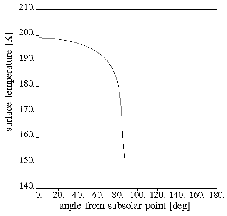
Figure 2: Equilibrium surface temperature versus the angle $\vartheta_{s}$ from the sub-solar point as given by the solution of equation (1).

In this paper we use the expressions “flux” for the number of impacting particles of a given mass per unit area and time, “fluence” for the flux integrated over time, “total flux” for the flux of particles of all masses, and “total fluence” for the total flux integrated over time.

2 Coma Model

In the following we describe the coma model we use to determine the cometary dust flux on the Stardust spacecraft. Because there is no standard model of the gas and dust environment of a comet nucleus, yet, we describe the assumptions and calculations we use in detail. So the reader can see how different assumptions or values of parameters change the results.

Since the dust is dragged into the coma by outflowing gas, we first have to calculate the gas density and velocity inside the coma. We assume that the outflow is symmetric about the Sun-nucleus axis. Therefore, all spatial distributions depend only on the angle $\vartheta_{s}$ between the considered location and the axis of symmetry and the radial distance $r$. We furthermore assume that the dust particles do not affect the gas flow, i.e. we use a test-particle approach.

2.1 Gas Phase

To calculate the state of the gas around the nucleus, we need to know the activity distribution on the nucleus’ surface, which is governed by the temperature distribution.

The temperature at a location on the day side of the nucleus’ surface is calculated such that there is an equilibrium between solar illumination, water sublimation, and blackbody reradiation. Therefore, the surface temperature $T_{s}(\vartheta_{s})$ is the solution of the following equation (the meaning and values of the parameters in the next two equations are given in table 1).

$$\begin{array}[]{l}\left(1-A_{B}\right)\left(\frac{f_{Sun}}{(r_{h}/1AU)}\right)^{2}\cdot\cos(\vartheta_{s})\\ \hskip 56.9055pt=\frac{L}{N_{A}}Z_{\rm HK}(T_{s}(\vartheta_{s}))+\epsilon\left(\sigma(T_{s}(\vartheta_{s}))\right)^{4},\end{array}$$ (1)

where $Z_{\rm HK}(T_{s})$ is the Hertz–Knudsen sublimation rate given by:

$$Z_{\rm HK}(T_{s}) = \frac{p(T_{s})}{\sqrt{2\pi m_{\rm H_{2}O}kT_{s}}}$$ (2)

We use the approximation $p(T_{s})=Ae^{(-B/T_{s})}$ for the vapor pressure [14].

Table 1: Parameters for computation of the surface temperature.

Solar constant	$f_{\rm Sun}=1370\;{\rm W}\;{\rm m}^{-2}$
nucleus surface albedo	$A_{B}=6\%$
Emissivity of comet surface	$\epsilon=1$
Boltzmann constant	$k=1.38\cdot 10^{-23}\;{\rm J}\;{\rm K}$
Stefan Boltzmann constant	$\sigma=5.67\cdot 10^{-7}\;{\rm W}\;{\rm K}^{-4}\;{\rm m}^{-2}$
Advogadro Number	$N_{A}=6\cdot 10^{23}{\rm mol}^{-1}$
Latent heat of water ice	$L=36\;{\rm kJ}\;{\rm mol}^{-1}$
Vapor pressure parameter	$A=3.56\cdot 10^{12}\;{\rm N}\;{\rm m}^{-2}$
Vapor pressure parameter	$B=6141\;{\rm K}$
1 bolometric Bond albedo

On the night side of the nucleus the temperature is constantly set to $150\;{\rm K}$. This value is also used at the day side near the terminator if the solution of equation (1) is smaller than $150\;{\rm K}$. Figure 2 shows the equilibrium temperature distribution determined from equation (1).

Figure 3: Solid lines represent lines of constant gas density (arbitrary units) in the region up to 25 comet radii ($=50\;{\rm km}$) around the nucleus. The Sun direction is upward and the short radial lines indicate the gas velocity (the scale on the top can be used to determine the modulus of the velocity). The gas density above the comet night side (bottom) is much lower than the density above the day side. However, the gas velocity above the day and night side is comparable. Apart from a region above the terminator, the gas flow is almost radial close to the nucleus.

Now, we obtain the activity $Q_{\rm HK}$ of the comet by inserting the temperature distribution into equation (2) and integrate over $\vartheta_{s}$.

$$Q_{\rm HK} = 2\pi r_{n}^{2}\int_{-1}^{1}Z_{\rm HK}(\vartheta_{s})d\cos(\vartheta_{s}).$$ (3)

In our model we use the outgasing activity of the nucleus given by Farnham and Schleicher (1997) [15]. On 1997 March 5 they report an $\rm OH$-activity $Q_{\rm OH}=5.9\cdot 10^{27}\;{\rm s}^{-1}$ and a value of the albedo–filling factor–radius product of $Af\rho=4.27\;{\rm m}$. At this time the comet was at a heliocentric distance of $1.7\;{\rm AU}$ and was observed at a phase angle of $27^{\circ}$. Although the observation was taken on the in-bound part of the comet’s orbit, and the Stardust spacecraft will approach the comet on the out-bound part, we assume that the observed activity is comparable to the comet’s activity during the encounter. Therefore, we run our coma model for a comet at $1.7\;{\rm AU}$ with a water activity equal to the observed $\rm OH$-activity $Q_{\rm H_{2}O}=5.9\cdot 10^{27}\;{\rm s}^{-1}$. To match the observed activity, the water sublimation rate is calculated by scaling the Hertz–Knudsen sublimation rate:

$$Z_{\rm H_{2}O}(\vartheta_{s}) = \frac{Q_{\rm H_{2}O}}{Q_{\rm HK}}\cdot Z_{\rm HK}(T_{s}(\vartheta_{s}))$$ (4)

In addition to the water activity, we assume a $\rm CO$-activity of $10\%$ of the water activity, i.e. $Q_{\rm CO}=5.9\cdot 10^{26}\;{\rm s}^{-1}$, and a constant distribution above the nucleus’ surface $Z_{\rm CO}(\vartheta_{s})=Q_{\rm CO}/(4\pi r_{n}^{2})$. For calculating the acceleration of the dust particles by the cometary gas, we have to consider the most abundant gas molecules only, therefore other constituents than $\rm H_{2}O$ and $\rm CO$ are not considered in the model and the total gas activity is set to $Q_{\rm gas}=Q_{\rm H_{2}O}+Q_{\rm CO}=6.5\cdot 10^{27}\;{\rm s}^{-1}$. Accordingly, we set the total gas activity distribution to $Z_{s}(\vartheta_{s})=Z_{\rm H_{2}O}(\vartheta_{s})+Z_{\rm CO}(\vartheta_{s})$. Using $Z_{s}(\vartheta_{s})$, the thermodynamic state of the gas can be determined by a numerical procedure described by Crifo et al. (1995) [8] and Knollenberg (1993) [29].

As an input to the calculation of the gas state we use a mean mass of a gas molecule of $m_{\rm gas}=(m_{\rm H_{2}O}Q_{\rm H_{2}O}+m_{\rm CO}Q_{\rm CO})$ $/(Q_{\rm H_{2}O}+Q_{\rm CO})$ and a mean degree of freedom per molecule of $f_{\rm gas}=(f_{\rm H_{2}O}Q_{\rm H_{2}O}+f_{\rm CO}Q_{\rm CO})/(Q_{\rm H_{2}O}+Q_{\rm CO})$. This simplification introduces some physical inconsistency into the model, but the results do not depend significantly on these choices.

Another important parameter for modeling the gas outflow is the initial gas temperature above the nucleus’ surface, because it determines the velocity reached by the gas, and therefore also has an impact on the dust acceleration. The initial gas temperature above the nucleus’ surface does not necessarily coincide with the surface temperature, because the gas is not at rest with respect to the surface. This effect was taken into account as it is described in Crifo and Rodionov (1997) [9] (Appendix B).

As shown in figure 3, the gas density determined by our thermodynamic model is distributed highly asymmetric around the nucleus. On the day side much more gas is available to accelerate dust from the surface. The flow direction is nearly radial. In the outer region of the coma, the gas is not dense enough to exert a significant drag force on the dust particles. We assume that the gas drag is negligible outside a maximum distance $r_{\rm max}$ of $25$ times the radius of the nucleus. After leaving this region, the dust particles move independently from the gas.

2.2 Dust Phase

The dust phase of a comet’s coma consists of all dust particles lifted and accelerated from the nucleus by the gas drag. The mass range of dust particles emitted by a comet covers many orders of magnitude and the dynamics of these particles depend on their mass. Therefore we divide the mass range $[10^{-20}\;{\rm kg},10^{0}\;{\rm kg}]$ into $20$ logarithmic mass decades $[m_{i-1},$ $m_{i}]$, $i=1,\ldots,20$ which we call “dust classes” in the following. All dust particles which are released with a mass inside one of the intervals $i$ are modeled by a dust particle of a representative mass $m_{d,i}$. We assume that no processes which change the properties of a dust particle, e.g. fractionation due to mutual collisions, take place after a particle has left the nucleus’ surface. Furthermore, we assume the dust particles to be spherical with a constant bulk density $\rho_{d}=1\;{\rm g}\;{\rm cm}^{-3}$ and a radius $s_{i}=(3m_{d,i}/(4\pi\rho_{d}))^{(1/3)}$. For the determination of the amount of dust in the coma, we derive a dust-to-gas mass ratio $\chi_{i}$ for each dust class. Using the dust to gas ratios $\chi_{i}$, we calculate the number of dust particles released per unit area and time.

$$Z_{d,i}(\vartheta_{s}) = \chi_{i}\frac{m_{\rm gas}}{m_{d,i}}Z_{\rm gas}(\vartheta_{s})$$ (5)

We take into account that particles cannot be lifted from the comet surface above a given mass by setting the dust activity to zero at locations on the comet surface where the gravitational attraction of the comet nucleus exceeds the drag force exerted by the gas.

To calculate the gravitational force of the nucleus, we determined the nucleus’ size by using ground-based observations of P/Wild 2 at large heliocentric distances. Fitzsimmons and Cartright (1995) [16] report a red magnitude of $R=22$ at the heliocentric distance of $r_{h}=4.4\;{\rm AU}$, a geocentric distance of $\Delta=4.0\;{\rm AU}$, and a phase angle of $\alpha=12^{\circ}$. We assume that P/Wild 2’s nucleus has a spherical shape. The radius of the nucleus $r_{n}$ can be calculated by (compare Jewitt (1991) [26])

$$r_{n} = r_{h}\frac{\Delta}{1\;{\rm AU}}\sqrt{\frac{10^{-0.4(R-R_{\rm Sun})}}{p_{\rm nuc}\cdot j_{\rm nuc}(\alpha)}},$$ (6)

where $R_{\rm Sun}=-27.22$ is the red magnitude of the Sun [35], $p_{\rm nuc}=4\%$ is used for the geometric albedo of the nucleus and $j_{\rm nuc}(\alpha)=10^{-0.4\delta\alpha}$ is the phase function of the nucleus with $\delta=0.035\;{\rm deg}^{-1}$ [26]. We find $r_{n}=2.3\;{\rm km}$. Because Fitzsimmons and Cartright (1995) [16] reported a ”near–stellar appearance”, there was already some contribution of the dust coma to the observed intensity. Therefore, $r_{n}=2.3\;{\rm km}$ is an overestimation of the radius of the nucleus and we use the value $r_{n}=2\;{\rm km}$ in our model.

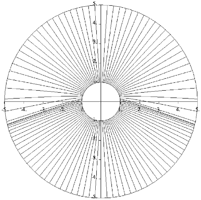
Figure 4: Trajectories of dust particles with radii of $8.8\;{\rm\mu m}$, which start at equidistant positions on the surface. The scales in the image are nucleus radii. The velocity of the particles is dominated by the radial component, far from the nucleus the tangential velocity component is negligible. The distance of the trajectories above the terminator is increased due to the tangential gas flow in this region.

Assuming a bulk density of $\rho_{n}=0.5\;{\rm g}\;{\rm cm}^{-3}$, the gravitational acceleration is given by:

$$\vec{a}_{\rm grav} = \mu_{n}\frac{\vec{r}}{\left|\vec{r}\right|^{3}}\hskip 14.22636pt\mbox{with}\hskip 14.22636pt\mu_{n}=1118\;{\rm m}^{3}\;{\rm s}^{-2}.$$ (7)

The acceleration of a dust particle due to gas drag can be expressed using the drag coefficient $C_{D}$:

$$\vec{a}_{\rm drag} = \frac{1}{2}m_{\rm gas}n_{\rm gas}\cdot\frac{\pi s_{i}^{2}}{m_{d,i}}C_{D}\left|\vec{v}_{\rm gas}-\vec{v}_{\rm dust}\right|$$ (8)

$$\cdot\left(\vec{v}_{\rm gas}-\vec{v}_{\rm dust}\right)$$

The drag coefficient in the free molecular approximation is given by Probstein (1968) [40]

$$C_{D} = \frac{2\sqrt{\pi}}{3s}\sqrt{\frac{T_{d}}{T_{\rm gas}}}+\frac{2s^{2}+1}{s^{3}\sqrt{\pi}}e^{(-s^{2})}$$ (9)

$$+\frac{4s^{4}+4s^{2}-1}{2s^{4}}\mbox{erf}(s),$$

where $s=|\vec{v}_{\rm gas}-\vec{v}_{dust}|/\sqrt{2kT_{\rm gas}/m_{\rm gas}}$. The dust temperature is set to $T_{d}=228\;{\rm K}$ (compare Divine (1981) [10]: $T_{d}=310\;{\rm K}\cdot(r_{h}/1\;{\rm AU})^{-0.58}$ and $r_{h}=1.7\;{\rm AU}$). At every point on the nucleus’ surface for which the gas drag acceleration exceeds the gravitational acceleration of the nucleus, the equation of motion of a dust particle can be solved numerically inside the gas flow (see figure 4 and 5). For large particles which can be lifted only from the comet’s day side, there are trajectories for which the radial velocity is not directed away from the nucleus but fall back into the nucleus’ direction (see figure 5). Since this behavior is only found in a narrow region, we do not consider these particles in the following.

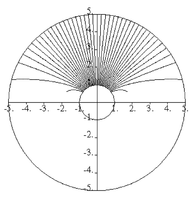
Figure 5: Trajectories of dust particles with a radius of $8.6\;{\rm mm}$. These big dust particles can only be lifted in a region around the sub-solar point. Near the boundary of this region there are trajectories which start to fall back in nucleus direction. In our model we neglect the contribution of these dust particles to the dust number density of the coma.

Apart from a narrow region near back-falling particles, the dust velocity is dominated by the radial velocity component. Since the contribution of the tangential velocity to the total dust velocity decreases with increasing distance from the nucleus’ surface, the dust trajectories can be approximated by straight radial lines with constant radial velocity at large distances. Outside the maximum distance $r_{\rm max}$ we approximate the dust trajectories by straight, radial lines and constant velocities $v_{e,i}(\vartheta)$ which is equal to the radial velocity computed for a dust particle at the distance $r_{\rm max}$. The angle $\vartheta$ denotes the angle of the position of the dust particle with respect to the Sun direction at $r_{\rm max}$, and is also the angle of the extrapolated trajectory with the Sun direction.

The dust number density outside the radius $r_{\rm max}$ can then be computed using the position $\vartheta_{s}$ of the trajectory at the nucleus’ surface as a function of the angle $\vartheta$ with respect to the Sun direction. To calculate the number density $n_{d,i}$ at positions with $r>r_{\rm max}$ and angle $\vartheta$, we introduce the activity distribution of the comet outside the acceleration zone:

$$Z_{e,i} = r_{n}^{2}Z_{s}(\vartheta_{s}(\vartheta))\frac{d\cos(\vartheta_{s})}{d\cos(\vartheta)}$$ (10)

For the number density $n_{d,i}$ we get:

$$n_{d,i}(r,\vartheta) = \frac{Z_{e,i}(\vartheta)}{r^{2}v_{e,i}(\vartheta)}$$ (11)

The number density inside the acceleration cone can be calculated in an analogous way.

As a result, we show the contours of constant dust particle density in figure 6. The region of high dust density occupies a larger volume on the day side than on the night side. Due to the drop in activity at the terminator, the dust particle density right above the terminator is lower than on the night side. Dust particles from the day side can propagate freely to the night side which extends the region of high dust particle density just behind the terminator in a narrow radial feature. If this is a real feature at a comet and if it can be observed in reality remains an open question. The dust particle density opposite to the Sun direction is the result of the night side activity.

Figure 6: The lines of constant dust number density of particles with radii of $8.8\mu m$ in the region within 25 radii of the nucleus. The radial lines indicate the velocity of the dust particles. Because of the low gas density, the dust particle velocity is smaller above the night side. Due to the increased tangential distance of the dust trajectories, the dust number density is small above the terminator (see figure 4).

We want to use the model to determine the dust flux on the Stardust instruments during the fly-by of the nucleus. We can neglect the influence of radiation pressure on the particle’s trajectories, because Stardust approaches the nucleus sufficiently close. Because the velocity of Stardust relative to nucleus is much larger than the velocity of the dust particles, the dust impact velocity at the spacecraft is dominated by the spacecraft’s motion. We therefore calculate the dust flux on the spacecraft by the product of the dust number density and the spacecraft velocity $v_{\rm SC}$ relative to the nucleus.

$$f_{\rm SC} = n_{d,i}\cdot v_{\rm SC}$$ (12)

From the result in equation (12) we can derive the dust fluence on the instruments, which is given by the time integral over the flux and represents the column density of dust particles along the spacecraft’s trajectory. We need the column density of dust particles also to calculate the brightness measured by an ground-based observer for a given line of sight.

As we show in Appendix A, the column density (in number of dust particles per ${\rm m}^{2}$) for an image plane with phase angle $\alpha$ can be calculated by

$$\frac{dn_{d,i}}{d(x^{\prime},y^{\prime})} = \frac{1}{\rho}\int_{-u}^{u}d\cos(\vartheta)\;\frac{Z_{e,i}(\vartheta)}{v_{e,i}(\vartheta)}$$ (13)

$$\cdot\frac{1}{\sqrt{u^{2}-\left(\cos(\vartheta)^{2}\right)}}N(\alpha,\eta,\vartheta),$$

where $u=u(\alpha,\eta)=\sqrt{1-(\sin(\eta)\cdot\sin(\alpha))^{2}}$. The variables $\rho$ and $\eta$ represent the position of the line of sight in the projected plane: $\rho$ is the distance from the (projected) nucleus position and $\eta$ denotes the direction of the line of sight position with anti-solar direction projected in the image plane (compare figure 20). $N(\alpha,\eta,\vartheta)$ is equal to the number of intersections of a line of sight with the cone of constant $\vartheta$ and is equal to $0$, $1$, or $2$ (see table 2).

Table 2: Number of intersections of a line of sight of angle $\eta$ with a cone of opening angle $\vartheta$ for different cases as explained in the text. Note that $(N(\alpha,\eta,\vartheta)+N(\alpha,\pi-\eta,\vartheta))/2=1$ for $|\cos(\vartheta)|<u$.

Condition 1	Condition 2	$N(\alpha,\eta,\vartheta)$
$u<\cos(\vartheta)$	none	$0$
$|\cos(\alpha)|<\cos(\vartheta)<u$	$\cos(\eta)<0$ $\cos(\eta)>0$	$2$ $0$
$\begin{array}[]{l}|\cos(\alpha)|>|\cos(\vartheta)>\\ -|\cos(\alpha)|\end{array}$	none	1
$-|\cos(\alpha)|>\cos(\vartheta)>-u$	$\cos(\eta)<0$ $\cos(\eta)>0$	$0$ $2$
$-u>\cos(\vartheta)$	none	$0$

For comparison with our axially symmetric model we provide the column density in the radially symmetric case:

$$\frac{dn_{d,i}}{d(x^{\prime},y^{\prime})} = \frac{\pi Z_{e,i}}{\rho v_{e,i}}.$$ (14)

2.3 Adjustment of the Dust Activity to the Observed $Af\rho$-value

We adjust the dust activity of our model so that the observed $Af\rho_{\rm obs}=4.27\;{\rm m}$ is matched. The $Af\rho$-parameter is related to the intensity $f_{\rm dust}$ received from dust particles inside a field of view with radius $\rho$ by A’Hearn et al. (1984) [1]:

$$Af\rho = 4\frac{\Delta^{2}(r_{h}/1AU)^{2}}{f_{\rm Sun}}\cdot\frac{f^{*}_{\rm dust}}{\rho},$$ (15)

where $f^{*}_{\rm Sun}$ is the radiation flux density of the Sun at a heliocentric distance of $1\;{\rm AU}$ observed in the same band of the spectrum as the comet, $\Delta$ is the geocentric distance and $r_{h}$ the heliocentric distance.

The intensity received due to a single dust particle is given by

$$I_{sng,i} = pj(\alpha)\cdot\frac{\pi s_{i}^{2}}{\pi\Delta^{2}}\cdot\frac{f^{*}_{\rm Sun}}{(r_{h}/1AU)^{2}},$$ (16)

where $p$ is the dust geometric albedo and $j(\alpha)$ is the dust phase function of the phase angle $\alpha$. Using the number of dust particles inside the aperture $N_{d,i}$ (see equation (38)), we can determine the $Af\rho$-parameter of our model by

$$Af\rho_{\rm mod} = 4pj(\alpha)\sum_{i}s_{i}^{2}\int_{0}^{2\pi}\int_{-u}^{u}\frac{Z_{e,i}(\vartheta)}{V_{e,i}(\vartheta)}$$ (17)

$$\cdot\frac{1}{\sqrt{u^{2}-\cos^{2}(\vartheta)}}d\cos(\vartheta)\;d\eta.$$

Here we assume that all dust particles have a geometric albedo and a phase function independent of size. For the geometric albedo we assume a value of $4$% and take the phase function from Divine (1981) [10].

To match the observed $Af\rho_{\rm obs}$ with the coma model, we have to scale the dust activity of the comet, i.e. the dust to gas ratio of all dust classes have to be scaled by the factor $Af\rho_{\rm obs}/Af\rho_{\rm mod}$.

2.4 Dust Mass Distribution

The mass distribution of the dust particles is the most crucial parameter of the model, because a change in the mass distribution can change the total dust fluence by orders of magnitude. Therefore we take special care to choose a reasonable mass distribution. In this section we explain our choice and discuss the resulting fluence in comparison with the measured fluence in the coma of P/Halley. The reader might want to check what the effects of a different choice of the mass distribution are.

The VEGA spacecraft measured the number of particles per unit area as a function of mass. We use this measurement as the mass distribution of our model. As an analytical representation of the mass distribution, we use a fit by Divine and Newburn (1987) [11].

$$F(m) = F_{t}\left(\frac{(1+x)^{b-1}}{x^{b}}\right)^{ac}\hskip 14.22636pt$$

$$\mbox{with}\hskip 14.22636ptx=\left(\frac{m}{m_{t}}\right)^{1/c}.$$

The parameters which fit the cumulative mass distribution of the VEGA 2 fluence best are $a=0.9$, $b=0.29$, $c=2.16$, and $m_{t}=1.6\cdot 10^{-13}\;{\rm kg}$ [11]. Since the mass distribution is only used to determine the relative but not the total abundance of particles in different dust classes, $F_{t}$ can be set to an arbitrary value. Note that $-a=-0.9$ is the exponent of the cumulative mass distribution for big dust particles ($m\gg m_{t},x\gg 1$), and $-ac=-1.9$ is the exponent for small particles ($m\ll m_{t},x\ll 1$).

For each dust class $[m_{i-1},m_{i}],\;i=1,\ldots,20$ considered in the model, the fluence on the VEGA 2 spacecraft inside one of the mass bins is proportional to

$$n_{VG2,i} \propto F(m_{i-1})-F(m_{i})$$ (19)

The dust fluence on the VEGA 2 spacecraft can be modeled analogous to the fluence on Stardust. At closest approach, VEGA 2 was also far inside the envelope of the measured dust particles, therefore, the total fluence was dominated by direct particles.

Because of the dependency of the integrand in equation (13) on the dust escape velocity $v_{e,i}$, which, in turn, depends on the mass of the dust particle, the mass distribution of particles which hit the VEGA 2 instruments does not coincide with the mass distribution of particles at the nucleus’ surface, i.e. the distribution of $Z_{d,i}$. Therefore a correction has to be applied to the VEGA 2 fluence before it can be used as mass distribution at the nucleus’ surface. For this purpose we compute the dust escape velocities $v_{e,i,{\rm Halley}}$ for an analogous radially symmetric P/Halley model (The model parameters are $Q_{\rm H_{2}O}=6.8\cdot 10^{29}\;{\rm s}^{-1}$ (see Krankowsky (1986) [30], $Q_{\rm CO}=0\;{\rm s}^{-1}$, $r_{n}=5\;{\rm km}$; all other model parameters are not changed). The fluence of dust class $i$ is inversely proportional to the dust escape velocity $v_{e,i,Halley}$ for a radially symmetric coma model (see equation (14)). Therefore, the product $n_{srf,i}=n_{VG2,i}\cdot v_{e,i,{\rm Halley}}$ is proportional to the mass distribution at the comet’s surface and the dust-to-gas mass ratios of the dust classes can be computed by

$$\chi_{i} = \chi_{\rm aux}\frac{m_{d,i}n_{srf,i}}{\sum_{j}m_{d,j}n_{srf,j}},$$ (20)

where $\chi_{\rm aux}$ is an auxiliary dust to gas ratio. $\chi_{\rm aux}$ would have the meaning of the ratio of dust mass to gas mass released per unit time from the comet’s nucleus, if all dust classes could be lifted from the comet’s surface. Since there are dust classes which can not be lifted from the comet’s surface or can only be lifted inside some region around the sub-solar point, no physical interpretation can be linked to this number and is in fact only an auxiliary value needed during the computation.

3 Model of LIC Dust Traversing the Solar System

The impact parameters of interstellar particles on the dust collector and the CIDA target are determined by the impact direction and velocity of the particles, and also by the articulation of the spacecraft during the cruise phase. Since both is non-trivial, we separate the effects by discussing two different types of particles: (1) the reference particles as defined by the Stardust mission plan [25] which move on straight lines through the Solar System in a direction derived from Ulysses and Galileo data, and (2) larger particles coming from the same direction, but being deflected due to solar gravity. For the reference particles the change in impact parameters is caused only by the spacecraft’s trajectory and the articulation strategies defined in the mission plan for the cruise phase. Larger particles are mainly interesting for the dust-collector, because CIDA is unlikely to be hit by such a particle due to its small target area and the low abundance of these particles. Furthermore, larger particles can be more easily extracted from the aerogel, this extraction might be difficult for particles with sizes of about a few tenth of a micron. In the following we argue why the reference particles are a good approximation of the most abundant interstellar particles, which are to be measured with Stardust and why smaller interstellar particles are not expected to reach the spacecraft.

In general, the dynamics of a charged, massive dust-particle in the interplanetary environment can be described by

$$\ddot{\vec{r}} = -\gamma\left(1-\beta\right)\frac{M_{\odot}}{\left|\vec{r}\right|^{3}}+\frac{Q}{m}\left(\vec{v}_{\rm swf}\times\vec{B}\right).$$ (21)

This equation of motion takes into account gravity, radiation pressure, and the Lorentz force induced by the solar wind magnetic field. $\gamma$ is the coupling constant of gravity, $M_{\odot}$ is the solar mass and the parameter $\beta$ is defined as the ratio of the magnitudes of radiation pressure force and gravity. $Q$ is the equilibrium charge to which a dust-particle will be charged in the interplanetary radiation and plasma environment, $\vec{v}_{\rm swf}$ is the velocity vector of the particle, measured in the frame of the radially expanding solar wind, and $\vec{B}$ represents the solar wind magnetic field. In equation (21) drag forces like Poynting-Robertson drag and solar wind drag are neglected, because these drag forces are small and only have a long-term effect on particles on bound orbits. The dynamical parameters $\beta$ and $Q/m$ depend on the particle size and can be represented as functions of particle radius $a$, if we assume a spherical shape for the particles [23, 39].

3.1 Reference Particles

Physically, the reference particles are implemented by setting $\beta=1$ and $Q/m=0\ {\rm C}\ {\rm kg}^{-1}$. In this case the solution to equation (21) are trajectories along straight lines, i.e. $\dot{\vec{r}}=\vec{v}_{\infty,{\rm dust}}={\rm const.}$. Since the Ulysses measurements indicate that interstellar dust and gas are kinematically coupled, we set $\vec{v}_{\infty,{\rm dust}}=\vec{v}_{\infty,{\rm gas}}$ using the parameters derived for the gas by Witte et al. (1996) [44] Gustafson (1994) [23] calculated $\beta$ as a function of particle radius assuming a spherical shape and a composition like the astronomical silicates defined by Draine and Lee (1984) [12] (see figure 7). Using these calculations it was shown [33], that for $57\%$ of all interstellar particles measured by Ulysses and Galileo $|1-\beta|\leq 0.4$. If the particles are measured at about $2\ {\rm AU}$, this deviation from the reference behavior would change the impact angle by less than $15^{\circ}$, which is the uncertainty in the determination of the interstellar dust upstream direction from the Ulysses and Galileo measurements. The impact velocity will deviate by less than $30\%$ for these particles. Furthermore, the variation of impact direction and velocity due to electro-magnetic interaction of interstellar particles with the solar wind magnetic field ($Q/m\neq 0\ {\rm C}\ {\rm kg}^{-1}$) can be neglected if they have radii larger than $0.2\ {\rm\mu m}$.

Figure 7: The parameter $\beta$ as a function of particle radius $a$. Homogeneous, spherical particles with the optical constants of astronomical silicates have been assumed (see [23]).

3.2 Gravitational Particles

As shown in figure 7, $\beta\approx 1$ is not valid for large particles. Large interstellar particles ($m>10^{-12}\ {\rm g}$) are less abundant than smaller ($m<10^{-12}\ {\rm g}$) ones [5], so they are more important for the dust collector than for CIDA due to its larger surface area. If we neglect electro-magnetic effects, the trajectories are hyperbolae and the spatial density distribution of these particles can be calculated analytically (see equation (44) in Appendix A). Figure 8 shows this distribution as a grey-scale in the ecliptic plane. In this simple model the density enhancement of large particles due to gravitational focusing during the collection phase is less than a factor of $2$.

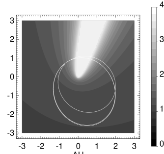
Figure 8: The normalized density distribution of gravitationally deflected ($\beta=0.1$) interstellar particles in the ecliptic plane represented by a grey-scale. The normalization is defined to set the spatial density at infinity equal to $1$. Stardust’s trajectory is indicated as the white solid line (compare to figure 1).

The enhancement in spatial density downstream the Sun is caused by gravitational focusing. Since the downstream vector of the interstellar dust flux has an angle of $\approx 5^{\circ}$ with respect to the ecliptic plane, the actual focus does not lie in the ecliptic, but a peripheral spatial density enhancement is present in the ecliptic plane. The main effect of the dynamics of large particles will be a higher impact velocity and a deviation in impact angle with respect to the reference particles.

Particles with large $\beta$-values ($\beta>1.4$) have diameters of $\approx 0.45\ {\rm\mu m}$ which correspond to the maximum wavelength of the solar spectrum. As we will argue in the next section, we do not expect these particles to be abundant in the Solar System during the Stardust mission due to their interaction with the solar wind magnetic field.

3.3 Electromagnetic Effects

In section 3.1 we have argued that electromagnetic effects can be neglected for the determination of the impact direction and velocity of interstellar particles. But we have to take into account these effects when considering the abundance of interstellar particles in the Solar System since long-term effects might reduce or enhance their spatial density. It was argued by Levy and Jokipii (1976) [36] that classical (very small) interstellar particles are removed from the Solar System by Lorentz force. The Ulysses and Galileo measurements show [5] a depletion of small particles (but still one order of magnitude above the detection threshold). Models of the electromagnetic interaction of the charged interstellar particles with the solar wind magnetic field [21, 24, 19] predict a periodic focusing and defocusing of the particles to the solar equator plane with the $22$-years solar cycle. A new magnetic cycle starts at solar maximum and the mean deflection effect is strongest when the magnetic field is in the most ordered configuration during the solar minimum. The last solar maximum in 1991 started a defocusing cycle. We have calculated the total flux of interstellar particles on the Ulysses detector as a function of time to check if the defocusing causes the total flux to drop. Figure 9 shows that the total flux (in the heliocentric inertial frame) of interstellar particles was constant after Ulysses’ fly-by of Jupiter in February 1992 (when Ulysses left the ecliptic plane).

Figure 9: Total flux $f$ of interstellar particles measured by Ulysses as a function of time. The error-bars are due to the fraction of particles which could not be clearly identified as interstellar dust.

The gap in the data between beginning and mid of 1995 is caused by the ecliptic crossing in March 1995 when distinction between interstellar and interplanetary particles was difficult. After mid of 1996 the measured total flux of interstellar particles drops by a factor of $3$. We interpret this phenomenon as the effect of electromagnetic defocusing. Unfortunately this can not be confirmed by Galileo data, because Galileo is inside the Jovian system since the end of 1995, therefore, Jupiter dust dominates the data and interstellar dust impacts can not be identified [31]. We assume that the period of reduced total flux will last for half a solar cycle, which is $11$ years, i.e. from mid of 1996 to mid of 2007. This period of time covers the duration of the Stardust mission. Following this estimate, we predict from the Ulysses data that the total dust flux on the Stardust experiments will be reduced by a factor of $3$ compared to the Ulysses and Galileo measurements.

For Ulysses and Galileo a total flux of $f_{\rm U/G}=1.5\cdot 10^{-4}$ ${\rm m}^{-2}\ {\rm s}^{-1}$ has been determined [3], so we predict $f_{\rm SD}=5\cdot 10^{-5}\ {\rm m}^{-2}\ {\rm s}^{-1}$.

4 Results

4.1 Cometary Dust Measurements

In this section we apply the coma model developed in section 2 to quantitatively predict the flux and the fluence of cometary dust particles on the Stardust spacecraft during the P/Wild 2 encounter. The results we obtain for an axially symmetric model are compared with the results we get if we use a radially symmetric model. We can compare our results for Stardust at P/Wild 2 with the fluence measured by the VEGA spacecraft inside the coma of P/Halley by scaling the predicted fluence with the difference in brightness, encounter distance, and phase angle.

Fluence as a function of mass

We approximate the trajectory of Stardust as a straight line passing the coma with a phase angle of $70^{\circ}$ with respect to the Sun direction. Stardust’s closest approach to the nucleus is above the comet’s day side. The fluence of dust particles of a given dust class $i$ during the whole trajectory is equal to the column density along the spacecraft’s trajectory which is given by equation (13). As the fluence is inversely proportional to the distance of closest approach of the spacecraft to the nucleus $\rho$, our results can easily be scaled to other closest approach distances. The numerical values of the fluence for a trajectory above the sub-solar point is given in table 3.

Flux and Fluence as a Function of Spacecraft Position

The fluence as a function of time from closest approach is calculated by the time integral, or, equivalently, by the integral over the path $s$ along the spacecraft’s trajectory, of the dust flux on the spacecraft as given in equation (12).

$$F_{SC,i}(t) = \int_{-\infty}^{V_{SC}t}f_{SC}\;dt=\int_{-\infty}^{s(t)}n_{d,i}(\vec{r}(s))\;ds$$ (22)

Table 3: Fluence of dust particles on the spacecraft for the radial and axially symmetric model for a closest approach distance of $\rho=100\;{\rm km}$. For different distances $\rho^{\prime}$ of closest approach the fluence can be scaled by $\rho/\rho^{\prime}$. In the axially symmetric model we assume that the spacecraft’s trajectory crosses the sub-solar point.

Dust	particle	particle
class	mass	radius	fluence $[{\rm m}^{-2}]$
$i$	$m_{d,i}\ [{\rm kg}]$	$s_{i}\ [{\rm m}]$	radial-symm.	axial-symm.
$1$	$10^{-20}$	$1.34\cdot 10^{-8}$	$5.86\cdot 10^{+07}$	$1.11\cdot 10^{+08}$
$2$	$10^{-19}$	$2.88\cdot 10^{-8}$	$3.86\cdot 10^{+07}$	$7.05\cdot 10^{+07}$
$3$	$10^{-18}$	$6.20\cdot 10^{-8}$	$2.52\cdot 10^{+07}$	$4.46\cdot 10^{+07}$
$4$	$10^{-17}$	$1.34\cdot 10^{-7}$	$1.60\cdot 10^{+07}$	$2.76\cdot 10^{+07}$
$5$	$10^{-16}$	$2.88\cdot 10^{-7}$	$9.67\cdot 10^{+06}$	$1.64\cdot 10^{+07}$
$6$	$10^{-15}$	$6.20\cdot 10^{-7}$	$5.39\cdot 10^{+06}$	$8.98\cdot 10^{+06}$
$7$	$10^{-14}$	$1.34\cdot 10^{-6}$	$2.58\cdot 10^{+06}$	$4.26\cdot 10^{+06}$
$8$	$10^{-13}$	$2.88\cdot 10^{-6}$	$9.37\cdot 10^{+05}$	$1.53\cdot 10^{+06}$
$9$	$10^{-12}$	$6.20\cdot 10^{-6}$	$2.32\cdot 10^{+05}$	$3.75\cdot 10^{+05}$
$10$	$10^{-11}$	$1.34\cdot 10^{-5}$	$4.11\cdot 10^{+04}$	$6.62\cdot 10^{+04}$
$11$	$10^{-10}$	$2.88\cdot 10^{-5}$	$6.02\cdot 10^{+03}$	$9.64\cdot 10^{+03}$
$12$	$10^{-09}$	$6.20\cdot 10^{-5}$	$8.11\cdot 10^{+02}$	$1.29\cdot 10^{+03}$
$13$	$10^{-08}$	$1.34\cdot 10^{-4}$	$1.06\cdot 10^{+02}$	$1.67\cdot 10^{+02}$
$14$	$10^{-07}$	$2.88\cdot 10^{-4}$	$1.37\cdot 10^{+01}$	$2.14\cdot 10^{+01}$
$15$	$10^{-06}$	$6.20\cdot 10^{-4}$	$1.78\cdot 10^{+00}$	$2.72\cdot 10^{+00}$
$16$	$10^{-05}$	$1.34\cdot 10^{-3}$	$2.40\cdot 10^{-01}$	$3.44\cdot 10^{-01}$
$17$	$10^{-04}$	$2.88\cdot 10^{-3}$	$3.55\cdot 10^{-02}$	$4.34\cdot 10^{-02}$
$18$	$10^{-03}$	$6.20\cdot 10^{-3}$	$6.31\cdot 10^{-03}$	$5.37\cdot 10^{-03}$
$19$	$10^{-02}$	$1.34\cdot 10^{-2}$	$0.00\cdot 10^{+00}$	$5.71\cdot 10^{-04}$
$20$	$10^{-01}$	$2.88\cdot 10^{-2}$	$0.00\cdot 10^{+00}$	$1.15\cdot 10^{-05}$

For a radially symmetric model an analytical expression is given by:

$$F_{SC,i} = \int_{-\infty}^{V_{SC}t}\frac{Z_{e,i}}{V_{e,i}\rho^{2}+s^{2}}\;ds$$ (23)

$$= \frac{Z_{e,i}}{V_{e,i}\rho}\cdot\left(\xi+\frac{\pi}{2}\right),$$

where $\xi=\arctan(V_{SC}t/\rho)$ is the angle of the spacecraft position to the point of closest approach. From equation (23) we see that $F_{SC,i}$ is a linear function of $\xi$ in the radially symmetric model.

We show the calculated total dust fluence on Stardust in figure 10.

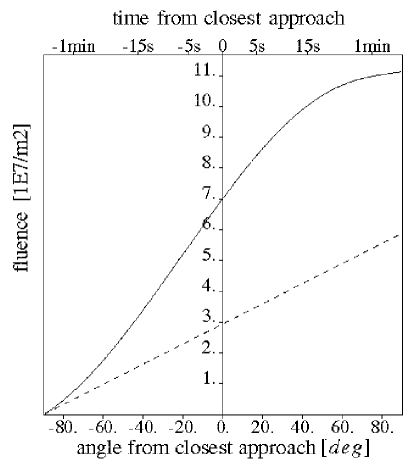
Figure 10: Total fluence on Stardust versus the angle $\xi$ from the location of closest approach for the radially symmetric (dashed line) and axially symmetric model (solid line). The total fluence calculated by the axially symmetric model deviates significantly from the result of the radially symmetric calculation.

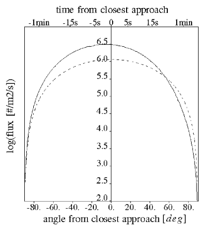
Figure 11: Total dust flux versus the angle $\xi$ between Stardust’s location on the trajectory and the location of closest approach P/Wild 2. The total flux of the axis and radially symmetric model are represented by the solid and dashed lines, respectively. It can be seen that the total flux predicted by the radially symmetric model is symmetric with respect to closest approach and reaches its maximum at that point.

In the axially symmetric model the total fluence is approximately a linear function of $\xi$ for $-40^{\circ}\leq\xi\leq 40^{\circ}$ , like it would be for the radially symmetric model. The radially symmetric model predicts a too low dust flux during closest approach, because it does not take into account the enhanced activity on the day side. Therefore, the slope of the total fluence is flatter between $\xi=-60^{\circ}$ and $\xi=60^{\circ}$ in the radially symmetric case. For $\xi>60^{\circ}$ Stardust enters the region above the terminator and consequently the total flux (and therefore the slope of the total fluence) drops below the value predicted by the radially symmetric model. We conclude that, for predicting the total dust fluence on Stardust during closest approach, one must take into account that Stardust approaches the comet from the day side and passes the terminator shortly after closest approach. The different results from the radially and axially symmmetric calculations show that the total fluence is strongly affected by the activity distribution on the surface of the nucleus. Unfortunately, we do not have any information about the activity distribution on P/Wild 2, so we have to rely on the axially symmetric coma model as a simple yet complete physical model of the inner coma for which we can constrain the parameters by measurements.

In figure 11 we show the total particle flux versus $\xi$. In the radially symmetric model the closest approach coincides with the point of highest total dust flux. Using the axially symmetric model, we find that the maximum total flux is reached $3\;{\rm s}$ before closest approach and that the total flux stays nearly constant until after closest approach. This is because the spacecraft enters into a region of lower activity after it has passed the sub-solar point but the decrease of cometary activity is apparently compensated by the still decreasing distance from the nucleus.

Reproduction of the VEGA and Giotto measurements at P/Halley

To validate our prediction of the fluence on the Stardust instruments, we scale our model to the conditions at P/Halley during the fly by of the Giotto and VEGA spacecraft. We stress that, although the VEGA 2 data were used to derive a mass distribution of our coma model, the comparison of the fluence is in fact a check of the model. This is because the VEGA 2 data were only used to derive the relative abundance of particles in different dust classes, but we derive the total amount of the dust activity from the value of $Af\rho$ that has been determined from ground based observations.

The fluence on the Stardust and VEGA spacecraft is proportional to the value of $Af\rho$ of the coma, inversely proportional to the distance $\rho$ of closest approach, and the dust phase function during the observation. Thus, the fluence which was computed for the Stardust spacecraft can be scaled to the fluence measured on board the VEGA spacecraft by multiplying the fluence with the following three ratios:

$$\begin{array}[]{ccccc}\lx@intercol\mbox{closest approach distance ratio:}\hfil\lx@intercol\\ \frac{\mbox{$\rho_{\mbox{\tiny Stardust}}$}}{\mbox{$\rho_{\mbox{\tiny VEGA}}$}}&\approx&\frac{100\;{\rm km}}{8000\;{\rm km}}&=&\frac{1}{80}\\ \\ \lx@intercol\mbox{$Af\rho$-ratio:}\hfil\lx@intercol\\ \frac{\mbox{$Af\rho_{\mbox{\tiny Halley}}$}}{\mbox{$Af\rho_{\mbox{\tiny Wild 2}}$}}&\approx&\frac{219\;{\rm m}}{4.27\;{\rm m}}&\approx&51.3\\ \\ \lx@intercol\mbox{dust phase function ratio:}\hfil\lx@intercol\\ \frac{\mbox{$j(\alpha_{\mbox{\tiny Wild 2}}\approx 30^{\circ})$}}{\mbox{$j\left(\alpha_{\mbox{\tiny Halley}}\approx 60^{\circ}\right)$}}&\approx&\frac{0.04}{0.032}&=&1.25\end{array}$$ (24)

The $Af\rho$ value of P/Halley during the VEGA encounter was taken from Schleicher et al. (1998) [41]. This leads to a total scaling factor of $51.3\cdot 1.25/80\approx 0.8$. Hence the fluence which we predict for Stardust at P/Wild 2 is compatible with the fluence measured on the VEGA spacecraft at P/Halley. In figure 12 we show the data of the fluence measured by VEGA together with the our prediction of the fluence on Stardust scaled by $0.8$.

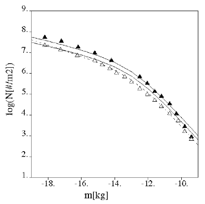
Figure 12: Fluence of dust particles on the VEGA spacecraft. Filled and outlined triangles represent VEGA 1 and VEGA 2 data, respectively. The fit to the VEGA 2 data by Divine and Newburn (1987) [11] is shown as the dashed line and the solid lines represent the scaled fluences as predicted by the axially symmetric (upper solid curve) and radially symmetric model (lower solid curve)

The good agreement of the number of dust particles collected on the VEGA spacecraft with the scaled Stardust fluence validates our procedure to derive the total dust activity of the comet from the observations and it shows that the parameter set we use in our model is consistent.

Unfortunately, because of the loss of the Giotto data near closest approach due to large particle impacts, we can not perform any quantitative comparison of the Giotto fluence to our model. However, we can estimate the total mass fluence on Giotto on the basis of the well known deceleration of $\Delta V=23\;{\rm cm}\;{\rm s}^{-1}$ [13] of Giotto during the encounter. As for the considered mass distribution, the total fluence is dominated by large particles and the momentum enhancement factor is believed to be rather low for large particles [13], the total mass fluence is estimated by assuming inelastic dust particle impacts on Giotto: With the Giotto mass of $M_{\rm Giotto}=573.7\;{\rm kg}$ and the velocity of $V_{\rm Giotto}=68.37\;{\rm km}\;{\rm s}^{-1}$ during encounter, the total mass which hit Giotto can be estimated to be $m_{\rm Giotto}=M_{\rm Giotto}/$ $V_{\rm Giotto}\cdot\Delta V\approx 2\;{\rm g}$. Using the area of the Giotto dust shield of $A=2.64\;{\rm m}^{2}$, we determine the total mass fluence on Giotto to be $0.76\;{\rm g}\;{\rm m}^{-2}$. The total mass fluence on the Stardust at P/Wild 2 can also be scaled to the total mass fluence on Giotto at P/Halley by taking into account that the closest approach distance of Giotto was approximatively $600\;{\rm km}$. We find the values $0.038\;{\rm g}$ and $0.064\;{\rm g}$ for the radially symmetric and axially symmetric model, respectively. Thus, the extrapolation of the mass distribution which was fitted by Divine and Newburn (1987) [11] to the fluence on the VEGA 2 spacecraft to larger masses leads to an underestimation of the total mass fluence by about one order of magnitude when compared to the total mass fluence derived from the final impact on Giotto. We discuss this discrepancy and its significance in section 5.

4.2 Interstellar Dust Measurements

We predict the measurements of interstellar dust during the interplanetary cruise phase by both main instruments on-board Stardust, CIDA and the aerogel collector. Unlike in the case of the measurements at P/Wild 2, the geometry of the measurements of both instruments is different, because they are used at different parts of the interplanetary trajectory. Therefore, we discuss the predictions for both instruments separately.

CIDA

To comprehend the predictions we make for CIDA one has to understand the three attitude strategies which have been defined by the mission plan [25]. Since CIDA has a fixed position on Stardust, its pointing is determined by the spacecraft attitude. The overall strategy should be to choose the attitude in a way that a maximum number of interstellar particles are detected assuming that they all behave like the reference particles. But the more one optimizes the attitude, the more complicated the spacecraft operations will become during the cruise phase. Thus, a trade-off has to be found between maximum number of detected particles and operation complexity.

We now explain the three different attitude strategies defined in the mission plan. Figure 13 shows a simplified sketch of Stardust containing the high gain antenna defining the $+z$-direction , the solar panels, which lie in the $x$-$y$-plane and the CIDA field of view (FOV) in the $x$-$z$-plane.

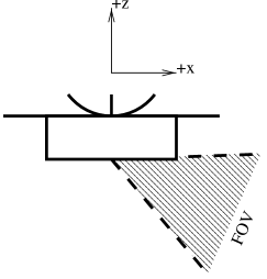
Figure 13: Configuration of the CIDA field of view (FOV) with respect to Stardust. The $+z$-direction is defined by the pointing of the high gain antenna and the fixed solar panels, which should always be pointed roughly towards the Sun.

In this plane the angle of FOV is $52^{\circ}$. Strategy #1 fixes the $+x$-axis to the upstream-direction of reference particles. This means that the $+z$ axis, i.e. the solar panels and the high gain antenna, are not always pointing to the Sun. The mission plan restricts this off-pointing to $45^{\circ}$ due to power concerns. If more than $45^{\circ}$ off-pointing is required to keep the $+x$-axis pointing upstream, the spacecraft is to be turned to full Sun-pointing again, which means that the upstream-direction is turned out of the FOV. Strategy #2 is the most complex one. If pointing of the $+x$-axis towards the upstream direction is possible without more than $45^{\circ}$ off-pointing of the $+z$-axis with respect to the Sun, strategy #2 is identical to strategy #1. But if this configuration is not possible any more, strategy #2 keeps the $45^{\circ}$ off-pointing as long as the upstream-direction lies inside the FOV. If even this is impossible, the spacecraft should return to Sun-pointing again. The most simple strategy is strategy #3. It fixes Sun-pointing of the $+z$-axis all the time, so CIDA will only collect interstellar particles when the upstream direction of the flux is occasionally in the FOV. Table 4 summarizes the three attitude strategies.

Table 4: Attitude strategies for the Stardust mission during the cruise phase as given by the mission plan.

strategy	description
# 1	$+x$-axis points upstream. Maximum Sun off-pointing is $45^{\circ}$.
# 2	upstream-direction is kept in the FOV. Maximum Sun off-pointing is $45^{\circ}$.
# 3	$+z$-axis always points towards the Sun.

Since the reference particles have a constant velocity of $26\;{\rm km}\;{\rm s}^{-1}$, the impact velocity of the reference particles as a function of time is determined by the spacecraft velocity. The impact velocity, the impact energy, and the quantity $mv_{i}^{3.5}$, which is proportional to the impact charge for impact plasma detectors [22], where $m$ is the mass and $v_{i}$ is the impact velocity of the particle, are shown in figure 14.

We predict the impact rate $\nu$ of reference particles on the CIDA target. We can estimate $\nu$ by the given effective sensitive target area of $A_{\rm CIDA}=80\ {\rm cm}^{2}\cdot\cos 40^{\circ}=60\;{\rm cm}^{2}$ [27], the flux $f_{\rm SD}=5\cdot 10^{-5}\;{\rm m}^{-2}\;{\rm s}^{1}$ (see section 3.3) in the inertial heliocentric frame, and the enhancement due to the upstream motion of Stardust. We get

$$\nu_{\rm max} = A_{\rm CIDA}f_{\rm SD}\left(\frac{v_{\rm rel,max}}{v_{\rm dust,ecl}}\right)\approx 7.0\cdot 10^{-7}\ {\rm s}^{-1},$$ (25)

where $v_{\rm rel,max}=60\ {\rm km}\ {\rm s}^{-1}$ is the maximum relative velocity of Stardust to the stream of reference particles (see above) and $v_{\rm dust,ecl}=26\ {\rm km}\ {\rm s}^{-1}$ is the velocity of the reference particles in the inertial ecliptic frame. Figure 15 shows the predicted impact rate on the CIDA target as a function of time for all three strategies explained above.

The total number of reference particles that CIDA will detect is given by the accumulated impact rate over time. We show the prediction in figure 16.

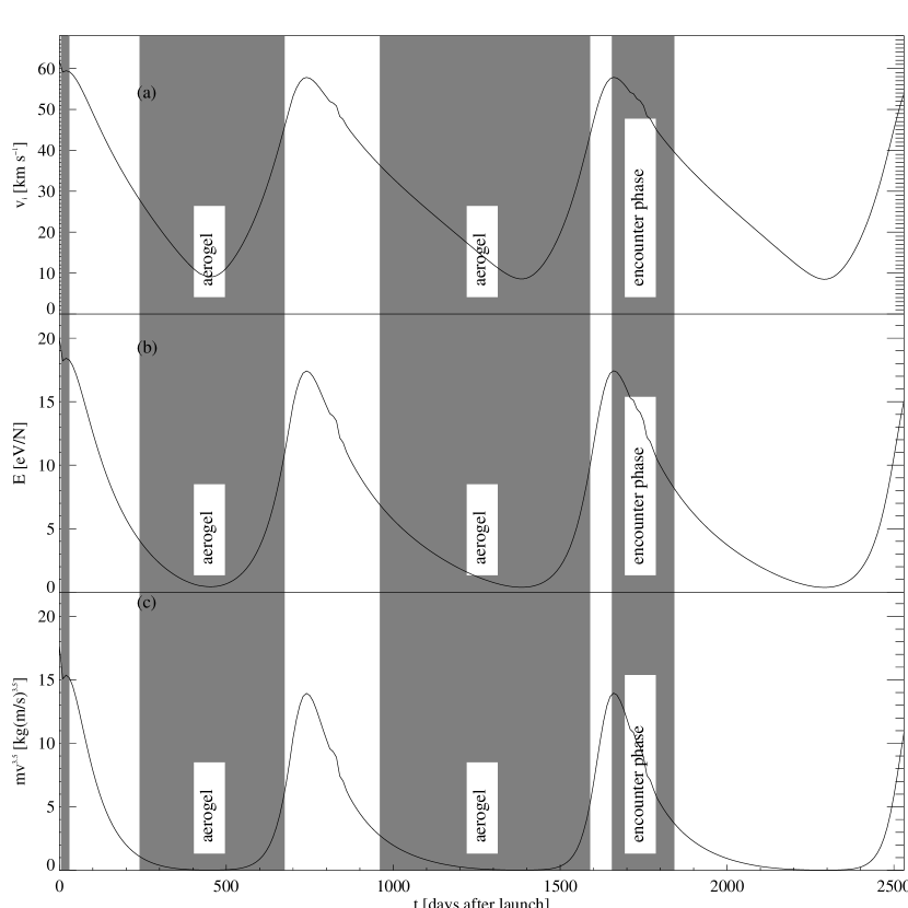
Figure 14: The values of $v$, $E=mv^{2}/2$, and $mv^{3.5}$ as a function of time, where $m$ is the mass and $v$ the velocity of the impacting reference particle. The shaded areas labeled “Arogel” indicate the phases of deployment of the Aerogel collector and “encounter Phases” labels the phase of preparations of the comet encounter. During these phases, CIDA is not taking data.

Figure 15: Impact rate on the CIDA target as a function of time. Prediction in panel (a) assumes strategy #1, in panel (b) strategy #2, and in panel (c) strategy #3. Mission phases during which CIDA is not allowed to be turned on due to other activities are indicated by the shaded areas (compare figure 14).

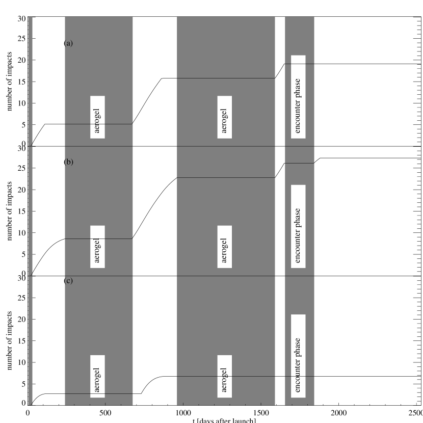
Figure 16: Total fluence on the CIDA target as a function of time. Prediction in panel (a) assumes strategy #1, in panel (b) strategy #2, and in panel (c) strategy #3. Mission phases during which CIDA is not allowed to be turned on due to other activities are indicated by the shaded areas (compare figure 14).

In summary, we predict that, assuming attitude strategy #2, CIDA will detect about $25$ particles which behave very much like reference particles and hit the target with velocities between $30\ {\rm km}\ {\rm s}^{-1}$ and $60\ {\rm km}\ {\rm s}^{-1}$ and energies between $18\;{\rm eV}\;{\rm N}^{-1}$ and $4\;{\rm eV}\;{\rm N}^{-1}$ (${\rm eV}\;{\rm N}^{-1}$ = electronvolt per nucleon). For a summary of the prediction see table 5, this table also contains the number of interplanetary dust particles as determined from the five-population model of interplanetary dust by Staubach et al. (1997) [42] “contaminating” the measurement.

Table 5: Number of interstellar and interplanetary particles predicted to be measured by Stardust during the cruise. For the collector we give the numbers for the front (which is exposed to the comet) and the back side (which is exposed to the interstellar upstream direction) seperately.

		collector
	CIDA	front	back
interstellar	$25$	$0$	$120$
interplanetary	$5$	$25$	$20$
1 Attitude strategy #2, see table 4

The Dust Collector

Figure 17: Total fluence on the aerogel detector of reference particles (a) and gravitationally deflected particles (b) as a function of time. Aerogel collection is not possible in the hatched periods.

Figure 18: Deviation of the impact angle of gravitationally deflected particles from the impact angle of reference particles, which should be close to $0^{\circ}$ as a function of time. Aerogel collection is not possible in the hatched regions.

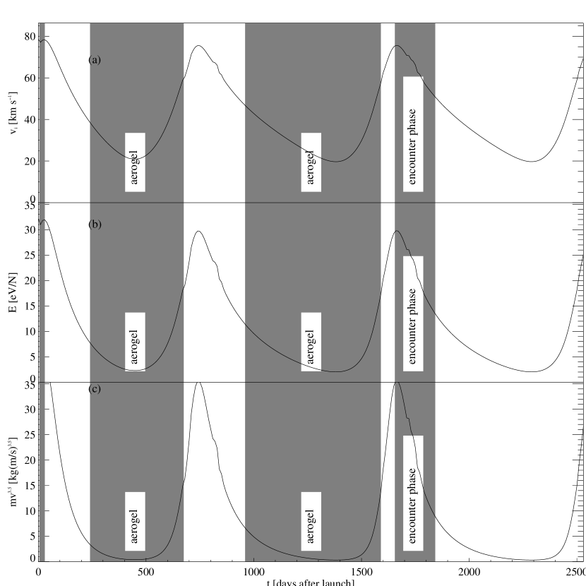
Figure 19: Values of $v$, $E=mv^{2}/2$, and $mv^{3.5}$ as a function of time, where $m$ is the mass and $v$ the velocity of the impacting gravitationally deflected particle (compare figure 14).

For the dust collector larger particles are more interesting, because their trajectories can more easily be measured and they can be extracted from the aerogel. Since the collector is turned to maintain a pointing to the upstream direction of the reference particles, we expect a spread in impact direction due to dynamical effects. For larger particles the dynamics should be dominated by gravity and we assume $\beta=0.1$ (see section 3.2). The Mie-calculations [23] give a radius of $1\ {\rm\mu m}$ for these particles, which translates to a mass of $1\cdot 10^{-11}\ {\rm g}$ assuming a density of $2.5\ {\rm g}\ {\rm cm}^{-3}$. In the Ulysses and Galileo data particles heavier than $10^{-11}\ {\rm g}$ make up $\approx 10\%$ of the total number [5], but they are not depleted due to electro-magnetic effects (see section 3.3). So we assume a flux of $1.5\cdot 10^{-5}\ {\rm m}^{-2}\ {\rm s}^{-1}$ of these large particles. We show the total fluence of interstellar particles on the collector for both, reference and gravitationally deflected particles, in figure 17.

Due to particle dynamics, tracks of larger particles should show a direction distribution. We show the deviation of impact angle as a function of time in figure 18.

For the collector it is furthermore interesting how fast gravitationally deflected particles impact into the aerogel. Since the particles are accelerated towards the Sun we expect their impact velocities to be higher than the impact velocities of the reference particles. In figure 19 we show the same plot as in figure 14 for gravitationally deflected particles.

To summarize our prediction for the aerogel collector, we give the total number particles collected during the $290$ days of exposure time [25] to be $120$. $80$ of these particles are small, like reference particles. The remaining $40$ are large particles, the impact tracks of which have angular deviations between $10^{\circ}$ and $30^{\circ}$. For the large particles we expect impact velocities on the aerogel between $20\ {\rm km}\ {\rm s}^{-1}$ and $40\ {\rm km}\ {\rm s}^{-1}$.

5 Discussion

We think that the Stardust mission to comet P/Wild 2 will enhance our understanding of the environment and the properties of comets by a large amount. According to our prediction, Stardust is able to fulfill its primary goal, the in situ measurement and collection of cometary dust particles. Concerning the secondary goal, the in situ detection and collection of interstellar dust particles from the local interstellar cloud, we find that the total number of particles we expect to be measured by Stardust is quite small considering the seven year duration of the mission. But having material from beyond the Solar System in a laboratory on the ground would be a big achievement.

We have determined the fluence on the Stardust spacecraft using a coma model. In our model the dust activity was determined using observations of P/Wild 2 at $1.7\;{\rm AU}$ heliocentric distance. Our model can reproduce the measurements of the VEGA spacecraft at P/Halley when scaling the model to the geometry of this measurement. The total mass fluence on Giotto, deduced from the fact that the spacecraft was hit by a very large particle, is underestimated by our model by one order of magnitude. Of course, a one-particle hit has not a very high statistic significance and we can hypothesize that this one hit was a low probability event. The possibility that the mass distribution used in our model has a deficit of large dust particles, as suggested by the DIDSY data [18], exists, but simply adding large particles to the mass distribution would either contradict ground based observations of the total brightness of P/Wild 2 during its in-bound part of its orbit at $1.7\;{\rm AU}$, or the dust fluence measured by VEGA at P/Halley. The real mass distribution of dust particles at the nucleus is still unknown and the reader may choose a different mass distribution and put it into our calculation to calculate the expected flux on Stardust.

Stardust approaches the comet from the sunlit side and therefore more dust particle impacts are expected before than after closest approach. Thus, a radially symmetric model is not sufficient to calculate the dust fluence on CIDA and the aerogel collector. As a result of the axially symmetric model, radial features on the night side of the nucleus appear (see figure 6). Unfortunately, we can not prove or disprove the existence of these features by the Stardust measurements, because Stardust is passing by the day side of P/Wild 2. The prove or disprove of the existence of such features remains a task for future ground based observations and space missions.

On the basis of the Galileo and Ulysses measurements we predict that during the interplanetary cruise phase $25$ mainly small ($m\approx 10^{-12}\ {\rm g}$) particles will hit the CIDA target. As the Ulysses data indicate, Stardust’s timing with the solar magnetic cycle is unfortunate (see section 3.3). To confirm that the decrease in the total flux of interstellar particles measured by Ulysses is due to their interaction with the solar wind magnetic field, modeling of this interaction is under way [33]. Even if the total number of interstellar particles detected by CIDA could be low, the scientific significance of the data, in any case, is high because the composition of LIC dust is to be directly measured for the first time by CIDA. The reliability of this measurement depends very much on the ability to identify interstellar impacts clearly. Interplanetary particles are a possible source of “contamination” for CIDA’s measurements. Table 5 shows that 5 interplanetary dust particles with masses greater than $10^{-14}\;{\rm g}$ are expected to hit the CIDA target during the cruise phase. For the determination of this number we have used the five-population-model of interplanetary dust by Staubach et al. (1997) [42]. So, interstellar particles should dominate the impacts on the CIDA target during cruise, but one has to make sure that an individual detection is really from an interstellar particle.

We expect the aerogel collector to contain about $120$ interstellar particles inside its interstellar collection layer. Of these, $40$ should be large particles (size $>1\ {\rm\mu m}$) that are probably the only ones which are extractable from the aerogel. Due to their high impact velocities, these large particles might be able to penetrate very deep into the aerogel and are possibly altered by the entry process. The distribution of impact angles can be determined by measuring the geometry of the entry-tracks. This will give valuable information on the dynamics of interstellar particles in the solar system. The highest amount of information is of course contained in the particles themselves when put into the laboratory and analyzed for their chemical and mineralogical properties. Like CIDA, the collector might also contain a contamination by interplanetary particles on both sides, the interstellar and the cometary dust collection layer. As shown in table 5 we predict $25$ interplanetary particles with masses greater than $10^{-13}\;{\rm g}$ to hit the cometary side of the collector and $20$ to hit the interstellar side.

If the interplanetary particles can be identified as such, it might be interesting to compare them with the IDPs collected by stratospheric aircraft [6, 38].

Appendix A Spatial Density in the Coma

The number of particles which leave the coma per unit time and solid angle is given by $Z_{e,i}(\vartheta)$, where $\vartheta$ denotes the angle between ejection and Sun direction. The velocity of the particles is given by $V_{e,i}(\vartheta)$. For the computation we introduce a reference frame with the comet nucleus in its origin: The z-axis is pointing to the anti-solar direction. The observers position is inside the z-x plane. The position of a particle which was released in the $(\vartheta,\varphi)$ direction before time $t$ with respect to this reference frame is given by (see figure 20):

$$\vec{r}(t,\vartheta,\varphi) = r\left(\begin{array}[]{c}\cos(\varphi)\sin(\vartheta)\\ -\sin(\varphi)\sin(\vartheta)\\ -\cos(\vartheta)\end{array}\right)\hskip 14.22636pt$$

$$\mbox{with}\hskip 14.22636ptr=tV_{e,i}(\vartheta)$$

The phase angle of the observation is denoted by $\alpha$. The projected position of a dust particle is given by (compare figure 20):

$$\begin{array}[]{l}\left(\begin{array}[]{c}x^{\prime}\\ y^{\prime}\end{array}\right)=\rho\left(\begin{array}[]{c}\cos(\eta)\\ \sin(\eta)\end{array}\right)\\ \hskip 28.45274pt=r\left(\begin{array}[]{c}-\cos(\alpha)\cos(\varphi)\sin(\vartheta)-\sin(\alpha)\cos(\vartheta)\\ -\sin(\varphi)\sin(\vartheta)\end{array}\right)\end{array}$$ (30)

The x-axis in the image plane is the projected anti-solar direction. Alternatively to the cartesian coordinates in the projected plane $(x^{\prime},y^{\prime})$ a point in the image plane can be represented by the cylindrical coordinates $(\rho,\eta)$, where the $\eta=0$ direction points towards the (projected) anti-solar direction. The number of particles which are ejected in the time interval $dt$ and with solid angles inside $d\varphi$ $\sin(\vartheta)d\vartheta$ is given by:

$$dN = Z_{e,i}(\vartheta)dt\,d\varphi\,\sin(\vartheta)d\vartheta$$ (31)

$$= \frac{Z_{e,i}(\vartheta)}{V_{e,i}(\vartheta)}dr\,d\varphi\,\sin(\vartheta)d\vartheta$$

Next, we determine the contribution of a cone of given angle $\vartheta$ to the projected number density is computed. The total number density is then obtained by integrating over all cones in a second step.

For computing the number of particles inside an infinitesimal area element in the projected plane $dA=\rho\,d\rho\,d\eta$ due to particles of the cone $\vartheta$, one needs to know for which radial distance $r$ and azimuthal angle $\varphi$ there are contributions to the chosen point in the image plane $(\rho,\eta)$. This can be found by solving equation (30) for $r$ and $\cos(\varphi)$ (with constant $\vartheta$). This leads to

$$r_{1,2} = \frac{\rho}{\cos^{2}(\vartheta)-\cos^{2}(\alpha)}\left(-\cos(\eta)\sin(\alpha)\cos(\vartheta)\right.$$ (32)

$$\left.\pm\cos(\alpha)\sqrt{u^{2}-\cos^{2}(\vartheta)}\right)$$

$$\cos(\varphi)_{1,2} = \frac{1}{u^{2}\sin(\vartheta)}\left(-\frac{\sin(2\alpha)\cos(\vartheta)}{2}\sin^{2}(\eta)\right.$$ (33)

$$\left.\pm\cos(\eta)\sqrt{u^{2}-\cos^{2}(\vartheta)}\right),$$

where $u=u(\alpha,\eta)=\sqrt{1-(\sin(\eta)\sin(\alpha))^{2}}$. For $u<|\cos(\vartheta)|$ the cone $\vartheta$ does not contribute to the point with angle $\eta$ in the image plane. Furthermore, since $r=V_{e,i}(\vartheta)t>0$, only the solutions with $r>0$ have to be considered. The number of solutions for a given angle $\eta$, phase angle $\alpha$, and cone $\vartheta$ is denoted by $N(\alpha,\eta,\vartheta)$ and is given for different conditions in table 2.

Finally, we calculate which infinitesimal azimuthal-radial element $dr\,d\varphi$ corresponds to the chosen surface element $dA=\rho\,d\rho\,d\eta$ in the image plane. This relation is given by the determinant of the Jacobian matrix:

$$\begin{array}[]{ccl}dN&=&\frac{Z_{e,i}(\vartheta)}{V_{e,i}(\vartheta)}\cdot\det\left(\begin{array}[]{cc}\frac{\partial r}{\partial\rho}&\frac{\partial r}{\partial\eta}\\ \frac{\partial\varphi}{\partial\rho}&\frac{\partial\varphi}{\partial\eta}\end{array}\right)\,d\rho\,d\eta\,\sin(\vartheta)d\vartheta\\ \\ &=&\frac{Z_{e,i}(\vartheta)}{V_{e,i}(\vartheta)}\cdot\left(\frac{\partial r}{\partial\rho}\cdot\frac{\partial\varphi}{\partial\eta}\right)\,d\rho\,d\eta\,\sin(\vartheta)d\vartheta\end{array}$$ (34)

Computation of the partial derivatives yields

$$dN=\frac{Z_{e,i}(\vartheta)}{V_{e,i}(\vartheta)}\frac{1}{\sqrt{u^{2}-\cos^{2}(\vartheta)}}d\rho\,d\eta\,\sin(\vartheta)d\vartheta.$$ (35)

Since the last equation gives only the contribution to the number density due to a single solution of equations (32) and (33) the contribution of all solutions has to be summed up to find the total number of particles in $dA=\rho\,d\rho\,d\eta$ due to cone $\vartheta$:

$$\frac{dN}{dA}=N(\alpha,\eta,\vartheta)\frac{Z_{e,i}(\vartheta)}{\rho V_{e,i}(\vartheta)}\frac{1}{\sqrt{u^{2}-\cos^{2}(\vartheta)}}\sin(\vartheta)d\vartheta$$ (36)

Finally, the projected number density is found by integrating over all cones which contribute to the chosen point $(\rho,\eta)$:

$$\frac{dn_{d,i}}{d(x^{\prime},y^{\prime})}(\rho,\eta) = \int_{-u}^{u}N(\alpha,\eta,\vartheta)\frac{Z_{e,i}(\vartheta)}{\rho V_{e,i}(\vartheta)}$$ (37)

$$\cdot\frac{1}{\sqrt{u^{2}-\cos^{2}(\vartheta)}}d\cos(\vartheta)$$

For the calculation of the intensity which is received from the dust coma the number of particles inside a circular field of view with radius $\rho$ is needed and can be found by integration of the projected number density over the field of view (note that $(N(\alpha,\eta,\vartheta)+N(\alpha,\pi-\eta,\vartheta))/2=1$):

$$N_{d,i}(\rho) = \rho\int_{0}^{2\pi}\int_{-u}^{u}\frac{Z_{e,i}(\vartheta)}{V_{e,i}(\vartheta)}$$ (38)

$$\cdot\frac{1}{\sqrt{u^{2}-\cos^{2}(\vartheta)}}d\cos(\vartheta)\;d\eta$$

Figure 20: We define the reference frame with the comet in its origin such that the $z$-axis points in the anti-solar direction and the observers position is located in the plane spanned by the $x$- and $z$-axis. In the projection plane, the $y^{\prime}$-axis is parallel to the y axis and the $x^{\prime}$-axis points in the direction of the projected anti-solar direction. Alternatively to the cartesian coordinates, a point in the projection plane can be represented by the cylindrical coordinates $(\rho,\eta)$, where $\rho$ is the distance of the point from the projected comet position and $\eta$ the angle from the anti-solar direction.

Appendix B Spatial Density of Hyperbolic Particles

We derive the number density of particles, which initially enter the Solar System on parallel trajectories with velocity $V_{\infty}$ and number density $n_{\infty}$, assuming that the particles are moving on Keplerian trajectories. For this purpose an infinitesimal volume element $dV$ at distance $r$ from the Sun and angle $\vartheta$ with respect to the direction the particles enter the Solar System is considered (see figure 21).

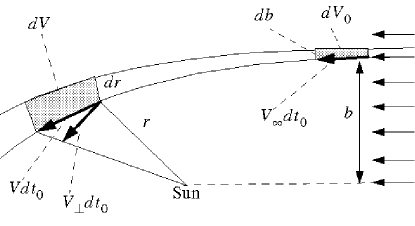
Figure 21: The sketch shows the volume element which contains the particles originating from the volume element $dV_{0}$. The particles on the right boundary of the volume elements reach the left boundary in the time $dt_{0}$.

The particles which cover the volume element $dV$ has started in the time interval $dt_{0}$ from outside the impact parameter interval $db$ and covered at a large distance from the Sun the volume element $dV_{0}=2\pi b\,db\,V_{\infty}dt_{0}$. The number of particles inside both volume elements is given by $dN=n_{\infty}\,dV_{0}$. The size of the volume element $dV$ can be computed by

$$dV=2\pi r\sin(\vartheta)\,dr\,V_{\bot}\,dt_{0}=2\pi r\,\frac{dr}{db}db\,V_{\bot}\,dt_{0}.$$ (39)

Due to the preservation of the angular momentum on a Keplerian trajectory the velocity perpendicular to the radial direction can be expressed by $V_{\bot}=bV_{\infty}/r$ and the size of the volume element can be written

$$dV=\sin(\vartheta)\frac{dr}{db}\,dV_{0}.$$ (40)

Thus, only the derivative of the radial distance $r$ with respect to the impact parameter needs to be computed. The radial distance $r$ of a non radial Keplerian trajectory can be parameterized:

$$r=\frac{p}{1+e\cos(\vartheta-\vartheta_{0})},$$ (41)

where $p$, $e$ and $\vartheta_{0}$ are constants which has to be expressed by the initial condition:

$$p = \frac{b^{2}}{d}$$

$$e = \pm\sqrt{1+\left(\frac{b}{d}\right)^{2}}$$

$$\cos(\vartheta_{0}) = -\frac{1}{e}$$

$$\sin(\vartheta_{0}) = \frac{b}{de}$$

$$d = \frac{\mu}{V_{\infty}^{2}},$$ (42)

where $\mu=\gamma M_{\odot}(1-\beta)$ is the effective gravitational constant of the Sun and $e$ is positive in the case $\mu>0$ and negative for $\mu<0$. By inserting the constants $p$, $e$ and $\vartheta_{0}$ in equation (41), we find the radial distance as a function of the impact parameter $b$:

$$r(b)=\frac{b^{2}}{d}\cdot\frac{1}{1-\cos(\vartheta)+\frac{b}{d}\sin(\vartheta)}$$ (43)

By computing the derivative with $b$ an expression for the number density at the position $(r,\vartheta)$ is found:

$$n=\frac{dN}{dV}=n_{\infty}\cdot\frac{b^{2}}{r\sin(\vartheta)|2b-r\sin(\vartheta)|}\hskip 28.45274pt\vartheta>0$$ (44)

For computing the number density at a given position in the Solar System, the impact parameter $b$ as a function of $r$ and $\vartheta$ is needed, what can be found by solving equation (43) for $b$:

$$b=\left|\frac{r\sin(\vartheta)}{2}\pm\sqrt{\left(\frac{r\sin(\vartheta)}{2}\right)^{2}+rd(1-\cos(\vartheta))}\right|$$ (45)

For an attractive effective gravitational constant $\mu>0$, i.e. $d>0$, every position can be reached by two trajectories (apart from the axes $\vartheta=0$ and $\vartheta=\pi$). For a repulsive effective gravitational constant $\mu<0$ i.e. $d<0$ every position outside the parabola $|r\sin(\vartheta)|=4\sqrt{d^{2}+d/2\cdot r\cos(\vartheta)}$ is reached by two different trajectories, no trajectories reach the interior of the parabola and every place on the parabola is reached by exactly one trajectory. Since equation (44) gives only the contribution to the number density of one solution the contributions due to the different solutions which reach a point has to be added up to calculate the total number density at a point. On the axis $\vartheta=\pi$ for $\mu>0$ and on the parabola for $\mu<0$ the volume element $dV$ becomes zero. Therefore the number density becomes infinite at those positions. However, the infinities are of that kind that any integral of the number density over a finite volume is finite.

Because the representation of a Keplerian orbit as it is given in equation (41) cannot be applied to radial trajectories i.e. impact parameter $b=0$ and $\vartheta=0$, the number density at the axis $\vartheta=0$ cannot be computed directly by equation (44), but the formula must be smoothly continued to this axis:

$$n=n_{\infty}\frac{1}{4}\left(\frac{1}{\sqrt{1+\frac{2d}{r}}}+\sqrt{1+\frac{2d}{r}}\pm 2\right),$$ (46)

The upper sign applies to the contribution to the number density due to the particles approaching the Sun and the lower sign to the departing particles.

References

- [1] A’Hearn, M. F., Schleicher, D. G., Millis, R.L., Feldmann, P.D., and Thompson, T.D., Comet Bowell 1980b, Astronomical Journal, 89, 579–591, 1984.
- [2] Albee, A. L., Brownlee, D. E., Burnett, D. S., Tsou, P., and Uesugi, K. T., Comet coma sample return instrument, in Lunar and Planetary Institute, Workshop on Particle Capture, Recovery and Velocity/Trajectory Measurement Technologies, pp. 5–7, 1994.
- [3] Baguhl, M., Grün, E., Hamilton, D. P., Linkert, G., Riemann, R., and Staubach, P., The flux of interstellar dust observed by Ulysses and Galileo, Space Science Reviews, 72, 471–476, 1995.
- [4] Baguhl, M., Hamilton, D., Grün, E., Dermott, S. F., Fechting, H., Hanner, M. S., Kissel, J., Lindblad, B.-A., Linkert, D., Linkert, G., Mann, I., McDonnell, J. A. M., Morfill, G. E., Polanskey, C., Riemann, R., Schwehm, G., Staubach, P., and Zook, H. A. , Dust measurements at high ecliptic latitudes, Science, 268, 1016–1019, 1995.
- [5] Baguhl, M., Grün, E., and Landgraf, M., In situ measurements of interstellar dust with the ulysses and galileo spaceprobes, in The Heliosphere in the Local Interstellar Medium, edited by R. von Steiger, R. Lallement, and M. Lee, vol. 78 of Space Science Reviews, pp. 165–172, Kluwer Academic Publishers, 1996.
- [6] Brownlee, D. E., Cosmic dust - collection and research, Annual Review of Earth and Planetary Sciences, 13, 147–173, 1985.
- [7] Brownlee, D. E., Tsou, P., Burnett, D., Clark, B., Hanner, M. S., Horz, F., Kissel, J., McDonnell, J. A. M., Newburn, R. L., Sandford, S., Sekanina, Z., Tuzzolino, A. J., and Zolensky, M., The Stardust mission: Returning comet samples to earth, Meteoritics & Planetary Science, 32, A22, 1997.
- [8] Crifo, J. F., Itkin, L., and Rodionov, A. V., The near-nucleus coma formed by interacting dusty gas jets effusing from a cometary nucleus I., Icarus, 116, 77–112, 1995.
- [9] Crifo, J. F. and Rodionov, A. V., The dependence of the circumnuclear coma structure on the properties of the nucleus, I. Comparison between homogeneous and an inhomogeneous spherical nucleus with application to P/Wirtanen, Icarus, 127, 319–353, 1997.
- [10] Divine, N., A simple radiation model of cometary dust of P/Halley, ESA SP-174, 25–30, 1981.
- [11] Divine, N. and Newburn, R. L., Modelling Halley before and after encounters, Astronomy and Astrophysics, 187, 867–872, 1987.
- [12] Draine, B. T. and Lee, H. M., Optical propoerties of interstellar graphite and silicate grains, Astrophysical Journal, 285, 89–108, 1984.
- [13] Edenhofer, P., Bird, M.K., Brenkle, J.P., Buschert, H., Kursinski, E.R., Mottinger, N.A., Porsche, H., Stelzried, C.T., and Volland, H., Dust distribution of comet P/Halley’s inner coma determined from the Giotto radio-science Experiment, Astronomy and Astrophysics, 187, 712–718, 1987.
- [14] Fanale F. P. and Salvail, J. R., An idealized short-period comet model: Surface insolation, flux, dust flux, and mantle evolution, Icarus, 60, 476–511, 1984.
- [15] Farnham, T., Schleicher, D., Hornoch, K., Znojil, V., Pereira, A., Bortle, J.E., and Granslo, B.H., Comet 81P/Wild 2, IAU Circ., 6597, 2, 1997.
- [16] Fitzsimmons, A. and Cartright, M., Comet 81P/Wild 2, IAU Circ., 6217, 1995.
- [17] Frisch, P. C., Characteristics of nearby interstellar matter, Space Science Reviews,72, 499–592, 1995.
- [18] Fulle M., Colangeli L., Mennella V., Rotundi A., and Bussoletti E., The sensitivity of the size distribution to the grain dynamics: simulation of the dust flux measured by Giotto at P/Halley, Astronomy and Astrophysics, 304, 622–630, 1995.
- [19] Grogan, K., Dermott, S. F., and Gustafson, B. Å. S., An estimation of the interstellar contribution to the zodiacal thermal emission, Astrophysical Journal, 472, 812–817, 1996.
- [20] Grün, E., Zook, H. A., Baguhl, M., Balogh, A., Bame, S. J., Fechtig, H., Forsyth, R., Hanner, M. S., Horanyi, M., Kissel, J., Lindblad, B.-A., Linkert, D., Linkert, G., Mann, I., McDonnell, J. A. M., Morfill, G. E., Phillips, J. L., Polanskey, C., Schwehm, G., Siddique, N., Staubach, P., Svestka, J., and Taylor, A., Discovery of jovian dust streams and interstellar grains by the Ulysses spacecraft, Nature, 362, 428–430, 1993.
- [21] Grün, E., Gustafson, B. Å. S., Mann, I., Baguhl, M., Morfill, G. E., Staubach, P., Taylor, A. , and Zook, H. A., Interstellar dust in the heliosphere, Astronomy and Astrophysics, 286, 915–924, 1994.
- [22] Grün, E., Baguhl, M., Fechtig, H., Kissel, J., Linkert, D., Linkert, G., and Riemann, R., Reduction of galileo and ulysses dust data, Planet. Space Sci., 43, 941–951, 1995.
- [23] Gustafson, B. Å. S., Physics of zodiacal dust, Annual Review of Earth and Planetary Science, 22, 553–95, 1994.
- [24] Gustafson, B. Å. S. and Lederer, S. M., Interstellar grain flow through the solar wind cavity around 1992, in Physics, Chemistry and Dynamics of Interplanetary Dust, edited by B. Gustafson and M. Hanner, vol. 104 of Astronomical Society of the Pacific Conference Series, pp. 35–39, 1996.
- [25] Hirst, E. H. and Yen, C.-W. L., Stardust mission plan, Tech. rep., Jet Propulsion Laboratory, 1997.
- [26] Jewitt, D., Cometary photometry, in Comets in the Post Halley Era, edited by R. L. Newburn, M. Neugebauer, and J. Rahe , volume 1, 19–65, 1991.
- [27] Kissel, J., pers. comm., 1997.
- [28] Kissel, J., Brownlee, D. E., Buchler, K., Clark, B. C., Fechtig, H., Grün, E., Hornung, K., Igenbergs, E. B,, Jeßberger, E. K., Krueger,F., Kuczera, H., McDonnell, J. A. M., Morfill, G. E., Rahe, J., Schwehm, G. H., Sekanina, Z., Utterback, N. G., Völk, H. J., and Zook, H. A., Composition of comet halley dust particles from Giotto observations, Nature, 321, 336–337, 1986.
- [29] Knollenberg, J., Modellrechnungen zur Staubverteilung in der inneren Koma von Kometen unter spezieller Berücksichtigung der [HMC-Daten der Giotto-Mission, Ph.D. thesis (in german), 1993.
- [30] Krankowsky, D. Lämmerzahl, P., Herrwerth, I., Woweries, J., Eberhardt, P., Polder, U., Herrmann, U., Schulte, W., Berthelier, J.J., Illiano, J.M., Hodges, R.R., and Hoffman J.H., In situ gas and ion measurements at comet Halley, Nature, 321, 326–329, 1986.
- [31] Krüger, H., Grün, E., Landgraf, M., Baguhl, M., Dermott, S. F., Fechtig, H., Gustafson, B. Å. S., Hamilton, D. P., Hanner, M. S., Horányi, M., Kissel, J., Lindblad, B. A., Linkert, D., Linkert, G., Mann, I., McDonnell, J. A. M., Morfill, G. E., Polanskey, C., Schwehm, G., Srama, R., and Zook, H. A., Three years of Ulysses dust data: 1993 to 1995, in press, 1998.
- [32] Lallement, R. and Bertin, P., Northern-hemisphere observations of nearby interstellar gas – possible detection of the local cloud, Astronomy and Astrophysics, 266, 479–485, 1992.
- [33] Landgraf, M., Modeling of the Dynamics and Interpretation of the In Situ Measurement of Interstellar Dust in the Local Vicinity of the Solar System, Ph.D. thesis, Ruprecht-Karls-Universität Heidelberg, 1998.
- [34] Landgraf, M. and Grün, E., In situ measurements of interstellar dust, in Proceedings of the IAU Colloquium No. 166 “The Local Bubble and Beyond”, edited by D. Breitschwerdt, M. Freyberg, and J. Trümper, vol. 506 of Lecture Notes in Physics, pp. 381–384, Springer Heidelberg, 1998.
- [35] Landolt-Börnstein, Numerical data and functional relationships in science and technology, in Astronomy and Astrophysics, Extension and Supplement to Volume 1, Subvolume a, ”Methods Constants Solar System”, Group VI Volume 2, 1981.
- [36] Levy, E. H. and Jokipii, J. R., Penetration of interstellar dust into the solar system, Nature, 264, 423–424, 1976.
- [37] Mazets, E.P., Sagdeev, R.Z., Aptekar, R.L., Golenetskii, S.V., Guryan, Yu.A., Dyachkov, A.V., Ilyinskii, V.N., Panov, V.N., Petrov, G.G., Savvin, A.V., Sokolov, I.A., Frederiks, D.D., Khavenson, N.G., Shapiro, V.D., and Shevchenko, V.I., Dust in comet P/Halley from VEGA observations, Astronomy and Astrophysics, 187, 699–706, 1987.
- [38] Love, S. G., Joswiak, D. J., and Brownlee, D. E., Densities of stratospheric micrometeorites., Icarus, 111, 227–, 1994.
- [39] Mukai, T., On the charge distribution of interplanetary grains, Astronomy and Astrophysics, 99, 1–6, 1981.
- [40] Probstein, R. F., The dusty gasdynamics of comet heads, in Problems in hydrodynamics and continuum mechanics, SIAM, 568–583, 1968.
- [41] Schleicher, D. G., Millis, R. L., Birch, P. V., Narrowband photometry of comet P/Halley: Variation with heliocentric distance, season and solar phase angle, Icarus, 132, 397–417, 1998.
- [42] Staubach, P., Grün, E., and Jehn, R., The meteoroid environment near earth, Advances in Space Research, 19(II), 301–308, 1997.
- [43] Witte, M., Rosenbauer, H., Banaszkiewicz, H., and Fahr, H., The Ulysses neutral gas experiment - determination of the velocity and temperature of the interstellar neutral helium, Advances in Space Research, 13, (6)121–(6)130, 1993.
- [44] Witte, M., Banaszkiewicz, M., and Rosenbauer, H., Recent results on the parameters of interstellar helium from the Ulysses/GAS experiment, in The Heliosphere in the Local Interstellar Medium, edited by R. von Steiger, R. Lallement, and M. Lee, vol. 78 of Space Science Reviews, pp. 289–296, Kluwer Academic Publishers, 1996.