Multiple mode gravitational wave detection with a spherical antenna

Abstract

Apart from omnidirectional, a solid elastic sphere is a natural multimode and multifrequency device for the detection of Gravitational Waves (GW). Motion sensing in a spherical GW detector thus requires a multiple set of transducers attached to it at suitable locations. Resonant transducers exert a significant back action on the larger sphere, and as a consequence the joint dynamics of the entire system has to be properly understood before reliable conclusions can be drawn from its readout. In this paper, we present and develop a mathematical formalism to analyse such dynamics, which generalises and enhances currently existing ones, and which clarifies their actual range of validity, thereby shedding light into the physics of the detector. In addition, the new formalism has enabled us to discover a new resonator layout (we call it PHC) which only requires five resonators per quadrupole mode sensed, and has mode channels, i.e., linear combinations of the transducers’ readouts which are directly proportional to the GW amplitudes. The perturbative nature of our proposed approach makes it also very well adapted to systematically assess the consequences of small mistunings in the device parameters by robust analytic methods. These prove to be very powerful, not only theoretically but also practically: confrontation of our model’s predictions with the experimental data of the LSU prototype detector TIGA reveals an agreement between both consistently reaching the fourth decimal place.

1 Introduction

The idea of using a solid elastic sphere as a gravitational wave (GW) antenna is almost as old as that of using cylindrical bars: as far back as 1971 Forward published a paper [Forward 1971] in which he assessed some of the potentialities offered by a spherical solid for that purpose. It was however Weber’s ongoing philosophy and practice of using bars which eventually prevailed and developped up to the present date, with the highly sophisticated and sensitive ultracryogenic systems currently in operation —see [Coccia et al.  1995b] and [Coccia et al. 1997] for reviews and bibliography. With few exceptions [Ashby & Dreitlein 1975, Wagoner & Paik 1977], spherical detectors fell into oblivion for years, but interest in them strongly re-emerged in the early 1990’s, and an important number of research articles have been published since which address a wide variety of problems in GW spherical detector science. At the same time, international collaboration has intensified, and prospects for the actual construction of large spherical GW observatories (in the range of $\sim$100 tons) are being currently considered in several countries , even in a variant hollow shape [Coccia et al. 1998].

A spherical antenna is obviously omnidirectional but, most important, it is also a natural multimode device, i.e., when suitably monitored, it can generate information on all the GW amplitudes and incidence direction [Magalhães et al. 1995], a capability which possesses no other individual GW detector, whether resonant or interferometric [Dhurandhar & Tinto 1989]. Furthermore, a spherical antenna could also reveal the eventual existence of monopole gravitational radiation, or set thresholds on it [Bianchi et al. 1998]. The theoretical explanation of these facts is to be found in the unique matching between the GW amplitude structure and that of the sphere oscillation eigenmodes: a general metric GW generates a tidal field of forces in an elastic body which is given in terms of the “electric” components $R_{0i0j}(t)$ of the Riemann tensor at its centre of mass by the following formula [Lobo 1995]:

$${\bf f}_{\rm GW}({\bf x},t)\ \ \ =\sum_{\stackrel{{\scriptstyle\scriptstyle l=0\ {\rm and}\ 2}}{{m=-l,...,l}}}\,{\bf f}^{(lm)}({\bf x})\,g^{(lm)}(t)$$ (1)

where ${\bf f}^{(lm)}({\bf x})$ are “tidal form factors”, while $g^{(lm)}(t)$ are specific linear combinations of the Riemann tensor components $R_{0i0j}(t)$ which carry all the dynamical information on the GW’s monopole ($l\/$ = 0) and quadrupole ($l\/$ = 2) amplitudes. It is precisely these amplitudes which a GW detector is aimed to measure.

On the other hand, a free elastic sphere has two families of oscillation eigenmodes, so called toroidal and spheroidal modes, and modes within either family group into ascending series of $l\/$-pole harmonics, each of whose frequencies is (2$l\/$+1)-fold degenerate —see [Lobo 1995] for full details. It so happens that only monopole and/or quadrupole spheroidal modes can possibly be excited by an incoming metric GW [Bianchi et al. 1996], and their GW driven amplitudes are directly proportional to the wave amplitudes $g^{(lm)}(t)$ of equation (1). It is this very fact which makes of the spherical detector such a natural one for GW observations [Lobo 1995]. In addition, a spherical antenna has a significantly higher absorption cross section than a cylinder of like fundamental frequency, and also presents good sensitivity at the second quadrupole harmonic [Coccia et al. 1995a].

In order to monitor the GW induced deformations of the sphere motion sensors are required. In cylindrical bars, current state of the art technology is based upon resonant transducers [Astone et al. 1993, Hamilton et al. 1989]. A resonant transducer consists in a small (compared to the bar) mechanical device possessing a resonance frequency accurately tuned to that of the cylinder. This frequency matching causes back-and-forth resonant energy transfer between the two bodies (bar and resonator), which results in turn in mechanically amplified oscillations of the smaller resonator. The philosophy of using resonators for motion sensing is directly transplantable to a spherical detector —only a multiple set rather than a single resonator is required if its potential capabilities as a multimode system are to be exploited to satisfaction.

A most immediate question in a multiple motion sensor system is: where should the sensors be? The answer to this basic question naturally depends on design and purpose criteria. Merkowitz and Johnson (M&J) made a very appealing proposal consisting in a set of 6 identical resonators coupling to the radial motions of the sphere’s surface, and occupying the positions of the centres of the 6 non-parallel pentagonal faces of a truncated icosahedron [Johnson & Merkowitz 1993, Merkowitz & Johnson 1995]. One of the most remarkable properties of such layout is that there exist 5 linear combinations of the resonators’ readouts which are directly proportional to the 5 quadrupole GW amplitudes $g^{(2m)}(t)$ of equation (1). M&J call these combinations mode channels, and they therefore play a fundamental role in GW signal deconvolution in a real, noisy system [Merkowitz 1998, Merkowitz, Lobo & Serrano 1999]. In addition, a reduced scale prototype antenna —called TIGA, for Truncated Icosahedron Gravitational Antenna— was constructed at Lousiana State University, and its working experimentally put to test [Merkowitz 1995]. The remarkable success of this experiment in almost every detail [Merkowitz & Johnson 1996, Merkowitz & Johnson 1997, Merkowitz & Johnson 1998] stands as a vivid proof of the practical feasibility of a spherical GW detector [Astone et al. 1997b].

Despite its success, the theoretical model proposed by M&J to describe the system dynamics is based upon a simplifying assumption that the resonators only couple to to the quadrupole vibration modes of the sphere [Johnson & Merkowitz 1993, Merkowitz & Johnson 1995]. While this is seen a posteriori of experimental measurements to be a very good approximation [Merkowitz 1995, Merkowitz & Johnson 1997], a deeper physical reason which explains why this happens is missing so far. The original motivation for the research we present in this article was to develop a new and more general approach for the analysis of the resonator problem, very much in the spirit of the methodology and results of reference [Lobo 1995]; this, we thought, would not only provide the necessary tools for a rigorous analysis of the system dynamics, but also contribute to improve our understanding of the physics of the spherical GW detector.

Pursuing this programme, we succeeded in setting up and solving the equations of motion for the coupled system of sphere plus resonators. The most important characteristic of our solution is that it is expressible as a perturbative series expansion in ascending powers of the small parameter $\eta^{1/2}$, where $\eta\/$ is the ratio between the average resonator’s mass and the sphere’s mass. The dominant (lowest) order terms in this expansion appear to exactly reproduce Merkowitz and Johnson’s equations [Merkowitz & Johnson 1995], whence a quantitative assessment of their degree of accuracy, as well as of the range of validity of their underlying hypotheses obtains; if further precision is required then a well defined procedure of going to next (higher) order terms is unambiguously prescribed by the system equations.

Beyond this, though, the simple and elegant algebra which emerges out of the general scheme has enabled us to explore different resonator layouts, alternative to the unique TIGA of M&J. In particular we have found one [Lobo & Serrano 1996, Lobo & Serrano 1997] requiring 5 rather than 6 resonators per quadrupole mode sensed and possessing the remarkable property that mode channels can be constructed from the system readouts, i.e., five linear combinations of the latter which are directly proportional to the five quadrupole GW amplitudes. We have called this distribution PHC —see below for full details.

The intrinsically perturbative nature of our approach makes it also particularly well adapted to assess the consequences of small defects in the system structure, such as for example symmetry breaking due to suspension attachments, small resonator mistunings and mislocations, etc. We have applied them with outstanding success to account for the reported frequency measurements of the LSU TIGA prototype [Merkowitz 1995], which was diametrically drilled for suspension purposes; in particular, discrepancies between measured and calculated values (generally affecting only the fourth decimal place) are precisely of the theoretically predicted order of magnitude.

We have also applied our methods to analyse the stability of the spherical detector to several mistuned parameters, with the result that it is not very sensitive to small construction errors. This conforms again to experimental reports [Merkowitz & Johnson 1998], but has the advantage that the argument depends on analytic mathematical work rather than on computer simulated procedures, the only ones available to this date to our knowledge —see e.g. [Merkowitz & Johnson 1998] or [Stevenson 1997].

The paper is structured as follows: in section 2 we present the main physical hypotheses of the model, and the general equations of motion. In section 3 we set up a Green function approach to solve those equations, and in section 4 we apply it to assess the system response to both monopole and quadrupole GW signals. In section 5 we describe in detail the PHC layout, including its frequency spectrum and mode channels. Section 6 contains a few brief considerations on the system response to a hammer stroke calibration signal, and finally in section 7 we study how the different parameter mistunings affect the detector’s behaviour. The paper closes with a summary of conclusions, and three appendices where the heavier mathematical details are made precise for the interested reader.

2 General equations

With minor improvements, we shall use the notation of references [Lobo 1995] and [Lobo & Serrano 1996], some of which is now briefly recalled. We consider a solid sphere of mass $\cal M\/$, radius $R\/$, (uniform) density $\varrho\/$, and elastic Lamé coefficients $\lambda$ and $\mu\/$, endowed with a set of $J\/$ resonators of masses $M_{a}\/$ and resonance frequencies $\Omega_{a}\/$ ($a\/$ = 1,…,$J\/$), respectively. We shall model the latter as point masses attached to one end of a linear spring, whose other end is rigidly linked to the sphere at locations ${\bf x}_{a}\/$ —see Figure 1. The system degrees of freedom are given by the field of elastic displacements ${\bf u}({\bf x},t)$ of the sphere plus the discrete set of resonator spring deformations $z_{a}(t)$; equations of motion need to be written down for them, of course, and this is our next concern in this section.

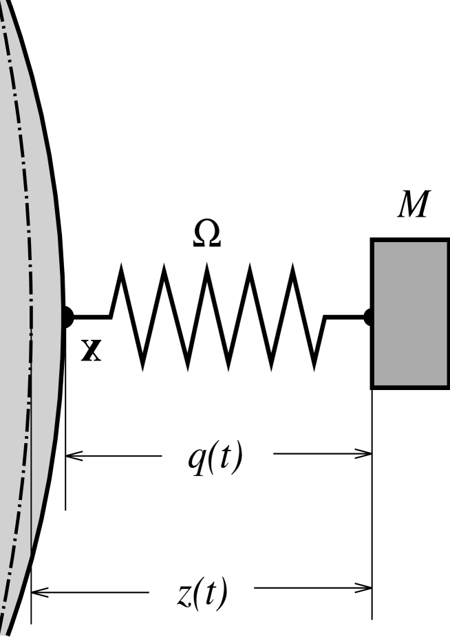
Figure 1: Schematic diagramme of the coupling model between a solid sphere and a resonator. The notation is that in the text, but subindices have been dropped for clarity. The dashed-dotted arc line on the left indicates the position of the undeformed sphere’s surface, and the solid arc its actual position.

We shall assume that the resonators only move radially, and also that Classical Elasticity theory [Landau & Lifschitz 1970] is sufficiently accurate for our purposes. In these circumstances we have [Lobo & Serrano 1996]

$$\varrho\,\frac{\partial^{2}{\bf u}}{\partial t^{2}} = \mu\nabla^{2}{\bf u}+(\lambda+\mu)\,\nabla(\nabla{\bf\cdot}{\bf u})+{\bf f}({\bf x},t)$$ (2)

$$\ddot{z}_{a}(t) = -\Omega_{a}^{2}\,\left[z_{a}(t)-u_{a}(t)\right]+\xi_{a}^{\rm external}(t)\ ,\qquad a=1,\ldots,J$$ (3)

where ${\bf n}_{a}\/$ $\equiv$ ${\bf x}_{a}/R\/$ is the outward pointing normal at the the $a\/$-th resonator’s attachment point, and

$$u_{a}(t)\equiv{\bf n}_{a}\!\cdot\!{\bf u}({\bf x}_{a},t)\ ,\qquad a=1,\ldots,J$$ (4)

is the radial deformation of the sphere’s surface at ${\bf x}_{a}\/$. A dot ( $\dot{}$ ) is an abbreviation for time derivative. The term in square brackets in (3) is thus the spring deformation —$q(t)$ in Figure 1.

${\bf f}({\bf x},t)$ in the rhs of (2) contains the density of all non-internal forces acting on the sphere, which we expediently split into a component due the resonators’ back action and an external action proper, which can be a GW signal, a calibration signal, etc. Thus

$${\bf f}({\bf x},t)={\bf f}_{\rm resonators}({\bf x},t)+{\bf f}_{\rm external}({\bf x},t)$$ (5)

Finally, $\xi_{a}^{\rm external}(t)$ in the rhs of (3) is the force per unit mass (acceleration) acting on the $a\/$-th resonator due to external agents.

Since we are making the hypothesis that the resonators are point masses the following holds:

$${\bf f}_{\rm resonators}({\bf x},t)=\sum_{a=1}^{J}M_{a}\Omega_{a}^{2}\,\left[\,z_{a}(t)-u_{a}(t)\right]\,\delta^{(3)}({\bf x}-{\bf x}_{a})\,{\bf n}_{a}$$ (6)

where $\delta^{(3)}\/$ is the three dimensional Dirac density function.

The external forces we shall be considering in this paper will be gravitational wave signals, and also a simple calibration signal, a perpendicular hammer stroke. GW driving terms, we recall from (1), can be written

$${\bf f}_{\rm GW}({\bf x},t)={\bf f}^{(00)}({\bf x})\,g^{(00)}(t)\ +\ \sum_{m=-2}^{2}\,{\bf f}^{(2m)}({\bf x})\,g^{(2m)}(t)$$ (7)

for a general metric wave —see [Lobo 1995] for explicit formulas and technical details. While the spatial coefficients ${\bf f}^{(lm)}({\bf x})$ are pure form factors associated to the tidal character of a GW excitation, it is the time dependent factors $g^{(lm)}(t)$ which carry the specific information on the incoming GW. The purpose of a GW detector is to determine the latter coefficients on the basis of suitable measurements.

If a GW sweeps the observatory then the resonators themselves will also be affected, of course. They will be driven, relative to the sphere’s centre, by a tidal acceleration which, since they only move radially, is given by

$$\xi_{a}^{\rm GW}(t)=c^{2}\,R_{0i0j}(t)\,x_{a,i}n_{a,j}\ ,\qquad a=1,\ldots,J$$ (8)

where $R_{0i0j}(t)$ are the “electric” components of the GW Riemann tensor at the centre of the sphere. These can be easily manipulated to give

$$\xi_{a}^{\rm GW}(t)=R\,\sum_{\stackrel{{\scriptstyle\scriptstyle l=0\ {\rm and}\ 2}}{{m=-l,...,l}}}\,Y_{lm}({\bf n}_{a})\,g^{(lm)}(t)\ ,\qquad a=1,\ldots,J$$ (9)

where $R\/$ is the sphere’s radius.

We shall also be later considering in this paper the response of the system to a particular calibration signal, consisting in a hammer stroke with intensity ${\bf f}_{0}$, delivered perpendicularly to the sphere’s surface at point ${\bf x}_{0}$:

$${\bf f}_{\rm stroke}({\bf x},t)={\bf f}_{0}\,\delta^{(3)}({\bf x}-{\bf x}_{0})\,\delta(t)$$ (10)

which we have modeled as an impulsive force in both space and time variables. Unlike GW tides, a hammer stroke will be applied on the sphere’s surface, so it has no direct effect on the resonators. In other words,

$$\xi_{a}^{\rm stroke}(t)=0\ ,\qquad a=1,\ldots,J$$ (11)

Our fundamental equations thus finally read:

$$\varrho\frac{\partial^{2}{\bf u}}{\partial t^{2}} = \mu\nabla^{2}{\bf u}+(\lambda+\mu)\,\nabla(\nabla{\bf\cdot}{\bf u})+$$ (12)

$$\sum_{b=1}^{J}M_{b}\Omega_{b}^{2}\,\left[z_{b}(t)-u_{b}(t)\right]\,\delta^{(3)}({\bf x}-{\bf x}_{b})\,{\bf n}_{b}+{\bf f}_{\rm external}({\bf x},t)$$

$$\ddot{z}_{a}(t) = -\Omega_{a}^{2}\,\left[z_{a}(t)-u_{a}(t)\right]+\xi_{a}^{\rm external}(t)\ ,\qquad a=1,\ldots,J$$ (13)

where ${\bf f}_{\rm external}({\bf x},t)$ will be given by either (7) or (10), as the case may be. Likewise, $\xi_{a}^{\rm external}(t)$ will be given by (9) or (11), respectively. The remainder of this paper will be concerned with finding solutions to the system of coupled differential equations (12) and (13), and with their meaning and consequences.

3 Green function formalism

In order to solve equations (12)-(13) we shall resort to Green function formalism. The essentials of this procedure in the context of the present problem can be found in detail in reference [Lobo 1995]; more specific technicalities are given in appendix A.

By means of such formalism equations (12)-(13) become the following integro-differential system:

$$u_{a}(t) = u_{a}^{\rm external}(t)+\sum_{b=1}^{J}\,\eta_{b}\,\int_{0}^{t}K_{ab}(t-t^{\prime})\,\left[\,z_{b}(t^{\prime})-u_{b}(t^{\prime})\right]\,dt^{\prime}$$ (14)

$$\ddot{z}_{a}(t) = \xi_{a}^{\rm external}(t)-\Omega_{a}^{2}\,\left[\,z_{a}(t)-u_{a}(t)\right]\ ,\qquad a=1,\ldots,J$$ (15)

where $u_{a}^{\rm external}(t)$ $\equiv$  ${\bf n}_{a}\!\cdot\!{\bf u}^{\rm external}({\bf x}_{a},t)$, and ${\bf u}^{\rm external}({\bf x},t)$ is the bare (i.e., without attached resonators) sphere’s response to the external forces ${\bf f}_{\rm external}({\bf x},t)$ in the rhs of (12). $K_{ab}(t)$ is a kernel matrix defined by the following weighted sum of diadic products of wavefunctions:

$$K_{ab}(t)=\Omega_{b}^{2}\,\sum_{N}\,\omega_{N}^{-1}\,\left[{\bf n}_{b}\!\cdot\!{\bf u}_{N}^{*}({\bf x}_{b})\right]\left[{\bf n}_{a}\!\cdot\!{\bf u}_{N}({\bf x}_{a})\right]\,\sin\omega_{N}t$$ (16)

Finally, we have defined the mass ratios of the resonators to the entire sphere

$$\eta_{b}\equiv\frac{M_{b}}{\cal M}\ ,\qquad b=1,\ldots,J$$ (17)

which will be small parameters in a real device.

Before proceeding further, let us briefly pause for a qualitative inspection of equations (14) and (15). Equation (14) shows that the sphere’s surface deformations $u_{a}(t)$ are made up of two contributions: one due to the action of external agents (GWs or other), contained in $u_{a}^{\rm external}(t)$, and another one due to coupling to the resonators. The latter is commanded by the small parameters $\eta_{b}\/$, and correlates to all of the sphere’s spheroidal eigenmodes through the kernel matrix $K_{ab}(t)$. This has consequences for GW detectors, for even though GWs may only couple to quadrupole and monopole spheroidal modes of the free sphere [Lobo 1995, Bianchi et al. 1996], attachment of resonators causes, as we see, coupling between these and the other modes of the antenna, and conversely, these modes back-act on the former. As we shall shortly prove, such effects can be minimised by suitable tuning of the resonators’ frequencies.

3.1 Laplace transform domain equations

We now take up the problem of solving these equations. Equation (14) is an integral equation belonging in the general category of Volterra equations [Tricomi 1957], but the usual iterative solution to it by repeated substitution of $u_{b}(t)$ into the kernel integral is not viable here due to the dynamical contribution of $z_{b}(t)$, which is in turn governed by the differential equation (15).

A better suited method to solve this integro-differential system is to Laplace-transform it. We denote the Laplace transform of a generic function of time $f(t)$ with a caret ( $\hat{}$ ) on its symbol, e.g.,

$$\hat{f}(s)\equiv\int_{0}^{\infty}f(t)\,e^{-st}\,dt$$ (18)

and make the assumption that the system is at rest before an instant of time, $t\/$ = 0, say, or

$${\bf u}({\bf x},0)={\bf\dot{u}}({\bf x},0)=z_{a}(0)=\dot{z}_{a}(0)=0$$ (19)

Equations (14) and (15) then adopt the equivalent form

$$\hat{u}_{a}(s) = \hat{u}_{a}^{\rm external}(s)-\,\sum_{b=1}^{J}\eta_{b}\,\hat{K}_{ab}(s)\,\left[\hat{z}_{b}(s)-\hat{u}_{b}(s)\right]$$ (20)

$$s^{2}\,\hat{z}_{a}(s) = \hat{\xi}_{a}^{\rm external}(s)-\Omega_{a}^{2}\,\left[\hat{z}_{a}(s)-\hat{u}_{a}(s)\right]\ ,\qquad a=1,\ldots,J$$ (21)

for which use has been made of the convolution theorem for Laplace transforms. A further simplification is accomplished if we consider that we shall in practice be only concerned with the measurable quantities

$$q_{a}(t)\equiv z_{a}(t)-u_{a}(t)\ ,\qquad a=1,\ldots,J$$ (22)

representing the resonators’ actual elastic deformations —cf. Figure 1. It is readily seen that these verify the following:

$$\sum_{b=1}^{J}\left[\delta_{ab}+\eta_{b}\,\frac{s^{2}}{s^{2}+\Omega_{a}^{2}}\,\hat{K}_{ab}(s)\right]\,\hat{q}_{b}(s)=-\frac{s^{2}}{s^{2}+\Omega_{a}^{2}}\,\hat{u}_{a}^{\rm external}(s)+\frac{\hat{\xi}_{a}^{\rm external}(s)}{s^{2}+\Omega_{a}^{2}}\ ,\qquad a=1,\ldots,J$$ (23)

Equations (23) constitute a significant simplification of the original problem, as they are a set of just $J\/$ algebraic rather than integral or differential equations. We must solve them for the unknowns $\hat{q}_{a}(s)$, then perform inverse Laplace transforms to revert to $q_{a}(t)$. We do this next.

4 System response to a Gravitational Wave

Our concern now is the actual system response when it is acted upon by an incoming GW. We shall calculate it by making a number of simplifying assumptions, more precisely:

1. The detector is perfectly spherical.

2. The resonators have identical masses and resonance frequencies.

3. The resonators’ frequency is accurately matched to one of the sphere’s oscillation eigenfrequencies.

As we shall see below (section 7), a real system can be appropriately treated as one which deviates by definite amounts from this idealised construct. Therefore detailed knowledge of the ideal system behaviour is essential for all purposes. This is the justification for the above simplifications.

The wavefunctions ${\bf u}_{nlm}({\bf x})$ of an elastic sphere can be found in reference [Lobo 1995] in full detail, and we shall keep the notation of that paper for them. The Laplace transform of the kernel matrix (16) can thus be expressed as —see equation (92) in appendix A:

$$\hat{K}_{ab}(s)=\sum_{nl}\,\frac{\Omega_{b}^{2}}{s^{2}+\omega_{nl}^{2}}\,\left|A_{nl}(R)\right|^{2}\,\frac{2l+1}{4\pi}\,P_{l}({\bf n}_{a}\!\cdot\!{\bf n}_{b})\equiv\sum_{nl}\,\frac{\Omega_{b}^{2}}{s^{2}+\omega_{nl}^{2}}\,\chi_{ab}^{(nl)}$$ (24)

where the last term simply defines the quantities $\chi_{ab}^{(nl)}$. Note that the sums here stretch across the entire spectrum of the solid sphere.

Our next assumption that all the resonators are identical simply means that

$$\eta_{1}=\,\ldots\,=\eta_{J}\equiv\eta\ ,\qquad\Omega_{1}=\,\ldots\,=\Omega_{J}\equiv\Omega$$ (25)

The third hypothesis makes reference to the fundamental idea behind using resonators, which is to have them tuned to one of the frequencies of the sphere’s spectrum. We express this by

$$\Omega=\omega_{n_{0}l_{0}}$$ (26)

where $\omega_{n_{0}l_{0}}$ is a specific and fixed frequency of the spheroidal spectrum.

In a GW detector it will only make sense to choose $l_{0}$ = 0 or $l_{0}$ = 2, as only monopole and quadrupole sphere modes couple to the incoming signal; in practice, $n_{0}$ will refer to the first or perhaps second harmonic [Coccia et al. 1995a]. We shall however keep the generic expression (26) for the time being in order to encompass all the possibilities with a unified notation.

Based on the above hypotheses, equation (23) can be rewritten in the form

$$\sum_{b=1}^{J}\,\left[\delta_{ab}+\eta\,\sum_{nl}\,\frac{\Omega^{2}s^{2}}{(s^{2}+\Omega^{2})(s^{2}+\omega_{nl}^{2})}\,\chi_{ab}^{(nl)}\right]\,\hat{q}_{b}(s)=-\frac{s^{2}}{s^{2}+\Omega^{2}}\,\hat{u}_{a}^{\rm GW}(s)+\frac{\hat{\xi}_{a}^{\rm GW}(s)}{s^{2}+\Omega^{2}}\ ,\qquad(\Omega=\omega_{n_{0}l_{0}})$$ (27)

where $\hat{\xi}_{a}^{\rm GW}(s)$ is the Laplace transform of (9), i.e.,

$$\hat{\xi}_{a}^{\rm GW}(s)=R\,\sum_{\stackrel{{\scriptstyle\scriptstyle l=0\ {\rm and}\ 2}}{{m=-l,...,l}}}\,Y_{lm}({\bf n}_{a})\,\hat{g}^{(lm)}(s)\ ,\qquad a=1,\ldots,J$$ (28)

As mentioned at the end of the previous section, we must now invert the matrix in the lhs of (27), which will give us an expression for $\hat{q}_{a}(s)$, then find the inverse Laplace transform of these functions to revert back to the time domain. A simple glance at the equation suffices however to grasp the unsurmountable difficulties of accomplishing this analytically.

Thankfully, though, a perturbative approach is applicable when the masses of the resonators are small compared to the mass of the whole sphere, i.e., when the inequality

$$\eta\ll 1$$ (29)

holds. We shall henceforth assume that this is the case, as also is with cylindrical bar resonant transducers. It is shown in appendix B that the perturbative series happens in ascending powers of $\eta^{1/2}$, rather than $\eta\/$ itself, and that the lowest order contribution has the form

$$\hat{q}_{a}(s)=\eta^{-1/2}\,\sum_{l,m}\,\hat{\Lambda}_{a}^{(lm)}(s;\Omega)\,\hat{g}^{(lm)}(s)+O(0)\ ,\qquad a=1,\ldots,J$$ (30)

where $O(0)$ stands for terms of order $\eta^{0}$ or smaller. Here, $\hat{\Lambda}_{a}^{(lm)}(s;\Omega)$ is a transfer function matrix which relates linearly the system response $\hat{q}_{a}(s)$ to the GW amplitudes $\hat{g}^{(lm)}(s)$, in the usual sense that $q_{a}(t)$ is given by the convolution product of the signal $g^{(lm)}(t)$ with the time domain expression, $\Lambda_{a}^{(lm)}(t;\Omega)$, of $\hat{\Lambda}_{a}^{(lm)}(s;\Omega)$. The detector is thus seen to act as a linear filter on the GW signal, whose frequency response is characterised by the properties of $\hat{\Lambda}_{a}^{(lm)}(s;\Omega)$. More specifically, the filter has a number of characteristic frequencies which correspond to the imaginary parts of the poles of $\hat{\Lambda}_{a}^{(lm)}(s;\Omega)$. As also shown in appendix B, these frequencies are the symmetric pairs

$$\omega_{a\pm}^{2}=\Omega^{2}\,\left(1\pm\sqrt{\frac{2l+1}{4\pi}}\,\left|A_{n_{0}l_{0}}(R)\right|\,\zeta_{a}\,\eta^{1/2}\right)+O(\eta)\ ,\qquad a=1,\ldots,J$$ (31)

where $\zeta_{a}^{2}\/$ is the $a\/$-th eigenvalue of the Legendre matrix

$$P_{l_{0}}({\bf n}_{a}\!\cdot\!{\bf n}_{b})\ ,\qquad a,b=1,\,\ldots,J$$ (32)

associated to the multipole ($l_{0}$) selected for tuning —see (26). These frequency pairs correspond to beats, typical of resonantly coupled oscillating systems —we shall find them again in section 6 in a particularly illuminating example.

Another very important fact is also neatly displayed by equation (30): the resonators’ motions are mechanically amplified by a factor $\eta^{-1/2}$ relative to the driving amplitudes $\hat{g}^{(lm)}(s)$. This is the counterpart, in our multimode system, of a similar behaviour known to happen in monomode cylindrical antennas [Astone et al. 1993].

The specific form of the transfer function matrix $\hat{\Lambda}_{a}^{(lm)}(s;\Omega)$ depends on both the selected mode to tune the resonator frequency $\Omega$, and on the resonator distribution geometry. We now come to a discussion of these.

4.1 Monopole gravitational radiation sensing

General Relativity, as is well known, forbids monopole GW radiation. More general metric theories, e.g. Brans-Dicke [Brans & Dicke 1961], do however predict this kind of radiation. It appears that a spherical antenna is potentially sensitive to monopole waves, so it can serve the purpose of thresholding, or eventually detecting them. This clearly requires that the resonator set be tuned to a monopole harmonic of the sphere, i.e.,

$$\Omega=\omega_{n0}\ ,\qquad(l_{0}=0)$$ (33)

where $n\/$ tags the chosen harmonic —most likely the first ($n\/$ = 1) in a thinkable device.

Since $P_{0}(z)$ $\equiv$ 1 (for all $z\/$) the eigenvalues of $P_{0}({\bf n}_{a}\!\cdot\!{\bf n}_{b})$ are, clearly,

$$\zeta_{1}^{2}=J\ ,\qquad\zeta_{2}^{2}=\,\ldots\,=\zeta_{J}^{2}=0$$ (34)

for any resonator distribution. The tuned mode frequency thus splits into a single strongly coupled pair:

$$\omega_{\pm}^{2}=\Omega^{2}\,\left(1\pm\sqrt{\frac{J}{4\pi}}\,\left|A_{n0}(R)\right|\,\eta^{1/2}\right)+O(\eta)\ ,\qquad\Omega=\omega_{n0}$$ (35)

The $\Lambda$-matrix of equation (30) is seen to be in this case

$$\hat{\Lambda}_{a}^{(lm)}(s;\omega_{n0})=(-1)^{J}\,\frac{a_{n0}}{\sqrt{J}}\,\frac{1}{2}\,\left[\left(s^{2}+\omega_{+}^{2}\right)^{-1}-\left(s^{2}+\omega_{-}^{2}\right)^{-1}\right]\,\delta_{l0}\,\delta_{m0}$$ (36)

whence the system response is

$$\hat{q}_{a}(s)=\eta^{-1/2}\,\frac{(-1)^{J}}{\sqrt{J}}\,a_{n0}\,\frac{1}{2}\,\left[\left(s^{2}+\omega_{+}^{2}\right)^{-1}-\left(s^{2}+\omega_{-}^{2}\right)^{-1}\right]\,\hat{g}^{(00)}(s)+O(0)\ ,\qquad a=1,\ldots,J$$ (37)

regardless of resonator positions. The overlap coefficient $a_{n0}$ is calculated by means of formulas given in [Lobo 1995], and has dimensions of length. By way of example, $a_{10}/R\/$ = 0.214, and $a_{20}/R\/$ = $-$0.038 for the first two harmonics.

A few interesting facts are displayed by equation (37). First, as we have already stressed, it is seen that if the resonators are tuned to a monopole detector frequency then only monopole wave amplitudes couple strongly to the system, even if quadrupole radiation amplitudes are significantly high at the observation frequencies $\omega_{\pm}\/$. Also, the amplitudes $\hat{q}_{a}(s)$ are equal for all $a\/$, as corresponds to the spherical symmetry of monopole sphere’s oscillations, and are proportional to $J^{-1/2}$, a factor we should indeed expect as an indication that GW energy is evenly distributed amongst all the resonators. A single transducer suffices to experimentally determine the only monopole GW amplitude $\hat{g}^{(00)}(s)$, of course, but (37) provides the system response if more than one sensor is mounted on the antenna for whatever reasons.

4.2 Quadrupole gravitational radiation sensing

We now consider the more interesting case of quadrupole motion sensing. We thus take

$$\Omega=\omega_{n2}\ ,\qquad(l_{0}=2)$$ (38)

where $n\/$ labels the chosen harmonic —most likely the first ($n\/$ = 1) or the second ($n\/$ = 2) in a practical system. The evaluation of the $\Lambda$-matrix is now considerably more involved [Serrano 1999], yet a remarkably elegant form is found for it:

$$\hat{\Lambda}_{a}^{(lm)}(s;\omega_{n2})=(-1)^{N}\,\sqrt{\frac{4\pi}{5}}\,a_{n2}\,\sum_{b=1}^{J}\,\left\{\sum_{\zeta_{c}\neq 0}\,\frac{1}{2}\left[\left(s^{2}+\omega_{c+}^{2}\right)^{-1}-\left(s^{2}+\omega_{c-}^{2}\right)^{-1}\right]\,\frac{v_{a}^{(c)}v_{b}^{(c)*}}{\zeta_{c}}\right\}\,Y_{2m}({\bf n}_{b})\,\delta_{l2}$$ (39)

where $v_{a}^{(c)}$ is the $c\/$-th normalised eigenvector of $P_{2}({\bf n}_{a}\!\cdot\!{\bf n}_{b})$, associated to the non-null eigenvalue $\zeta_{c}^{2}$. Let us stress that equation (39) explicitly shows that at most 5 pairs of modes, of frequencies $\omega_{c\pm}$, couple strongly to quadrupole GW amplitudes, no matter how many resonators in excess of 5 are mounted on the sphere. The tidal overlap coefficients $a_{2n}\/$ can also be calculated, and give for the first two harmonics [Lobo & Serrano 1996]

$$\frac{a_{12}}{R}=0.328\ ,\qquad\frac{a_{22}}{R}=0.106$$ (40)

The system response is thus

$$\hat{q}_{a}(s) = \eta^{-1/2}\,(-1)^{J}\,\sqrt{\frac{4\pi}{5}}\,a_{n2}\,\sum_{b=1}^{J}\,\left\{\sum_{\zeta_{c}\neq 0}\,\frac{1}{2}\left[\left(s^{2}+\omega_{c+}^{2}\right)^{-1}-\left(s^{2}+\omega_{c-}^{2}\right)^{-1}\right]\,\frac{v_{a}^{(c)}v_{b}^{(c)*}}{\zeta_{c}}\right\}\times$$ (41)

$$\hskip 113.81102pt\times\sum_{m=-2}^{2}\,Y_{2m}({\bf n}_{b})\,\hat{g}^{(2m)}(s)+O(0)\ ,\qquad a=1\,\ldots,J$$

Equation (41) is completely general, i.e., it is valid for any resonator configuration over the sphere’s surface, and for any number of resonators. It describes precisely how all 5 GW amplitudes $\hat{g}^{(2m)}(s)$ interact with all 5 strongly coupled system modes; like before, only quadrupole wave amplitudes are seen in the detector (to leading order) when $\Omega$ = $\omega_{n2}$, even if the incoming wave carries significant monopole energy at the frequencies $\omega_{c\pm}$.

The degree of generality and algebraic simplicity of (41) is new in the literature. As we shall now see, it makes possible a systematic search for different resonator distributions and their properties.

5 The PHC configuration

Merkowitz and Johnson’s TIGA [Johnson & Merkowitz 1993] is highly symmetric, and is the minimal set with maximum degeneracy, i.e., all the non-null eigenvalues $\zeta_{a}\/$ are equal. To accomplish this, however, 6 rather than 5 resonators are required on the sphere’s surface. Since there are just 5 quadrupole GW amplitudes one may wonder whether there are alternative layouts with only 5 resonators. Equation (41) is completely general, so it can be searched for an answer to this question. In reference [Lobo & Serrano 1996] we made a specific proposal, which we now describe in more detail.

In pursuing a search for 5 resonator sets we found that distributions having a sphere diameter as an axis of pentagonal symmetry exhibit a rather appealing structure. More specifically, let the resonators be located at the spherical positions

$$\theta_{a}=\alpha\qquad({\rm all}\,\ a)\ ,\qquad\varphi_{a}=(a-1)\,\frac{2\pi}{5}\ ,\qquad a=1,\ldots,5$$ (42)

The eigenvalues and eigenvectors of $P_{2}({\bf n}_{a}\!\cdot\!{\bf n}_{b})$ are easily calculated:

$$\zeta_{0}^{2}=\frac{5}{4}\,\left(3\,\cos^{2}\alpha-1\right)^{2}\ ,\qquad\zeta_{1}^{2}=\zeta_{-1}^{2}=\frac{15}{2}\,\sin^{2}\alpha\,\cos^{2}\alpha\ ,\qquad\zeta_{2}^{2}=\zeta_{-2}^{2}=\frac{15}{8}\,\sin^{4}\alpha$$ (43)

$$v_{a}^{(m)}=\sqrt{\frac{4\pi}{5}}\,\zeta_{m}^{-1}\,Y_{2m}({\bf n}_{a})\ ,\qquad m=-2,\ldots,2\ ,\ \ a=1,\ldots,5$$ (44)

so the $\Lambda$-matrix is also considerably simple in structure in this case:

$$\hat{\Lambda}_{a}^{(lm)}(s;\omega_{n2})=-\sqrt{\frac{4\pi}{5}}\,a_{n2}\,\zeta_{m}^{-1}\,\frac{1}{2}\left[\left(s^{2}+\omega_{m+}^{2}\right)^{-1}-\left(s^{2}+\omega_{m-}^{2}\right)^{-1}\right]\,Y_{2m}({\bf n}_{a})\,\delta_{l2}\qquad({\sl PHC})$$ (45)

where we have used the notation

$$\omega_{m\pm}^{2}=\Omega^{2}\,\left(1\pm\sqrt{\frac{5}{4\pi}}\,\left|A_{n2}(R)\right|\,\zeta_{m}\,\eta^{1/2}\right)+O(\eta)\ ,\qquad m=-2,\ldots,2$$ (46)

As we see from these formulas, the five expected pairs of frequencies actually reduce to three, so pentagonal distributions keep a certain degree of degeneracy, too. The most important distinguishing characteristic of the general pentagonal layout is best displayed by the explicit system response:

$$\hat{q}_{a}(s)=-\eta^{-1/2}\,\sqrt{\frac{4\pi}{5}}\,a_{n2} \left\{\,\frac{1}{2\zeta_{0}}\left[\left(s^{2}+\omega_{0+}^{2}\right)^{-1}-\left(s^{2}+\omega_{0-}^{2}\right)^{-1}\right]\,Y_{20}({\bf n}_{a})\,\hat{g}^{(20)}(s)\right.$$

$$+\;\frac{1}{2\zeta_{1}}\left[\left(s^{2}+\omega_{1+}^{2}\right)^{-1}-\left(s^{2}+\omega_{1-}^{2}\right)^{-1}\right]\,\left[Y_{21}({\bf n}_{a})\,\hat{g}^{(11)}(s)+Y_{2-1}({\bf n}_{a})\,\hat{g}^{(1\,-1)}(s)\right]$$

$$+\left.\frac{1}{2\zeta_{2}}\left[\left(s^{2}+\omega_{2+}^{2}\right)^{-1}-\left(s^{2}+\omega_{2-}^{2}\right)^{-1}\right]\,\left[Y_{22}({\bf n}_{a})\,\hat{g}^{(22)}(s)+Y_{2-2}({\bf n}_{a})\,\hat{g}^{(2\,-2)}(s)\right]\right\}$$

This equation indicates that different wave amplitudes selectively couple to different detector frequencies. This should be considered a very remarkable fact, for it thence follows that simple inspection of the system readout spectrum immediately reveals whether a given wave amplitude $\hat{g}^{2m}(s)$ is present in the incoming signal or not.

Pentagonal configurations also admit mode channels, which are easily constructed from (5) thanks to the orthonormality property of the eigenvectors (44):

$$\hat{y}^{(m)}(s)\equiv\sum_{a=1}^{5}\,v_{a}^{(m)*}\hat{q}_{a}(s)=\eta^{-1/2}\,a_{n2}\,\frac{1}{2}\left[\left(s^{2}+\omega_{m+}^{2}\right)^{-1}-\left(s^{2}+\omega_{m-}^{2}\right)^{-1}\right]\,\hat{g}^{(2m)}(s)+O(0)\ ,\qquad m=-2,\ldots,2$$ (48)

These are almost identical to the TIGA mode channels [Merkowitz & Johnson 1995], the only difference being that each mode channel comes now at a single specific frequency pair $\omega_{m\pm}$.

Mode channels are fundamental in signal deconvolution algorithms in noisy systems [Merkowitz 1998, Merkowitz, Lobo & Serrano 1999]. Pentagonal resonator configurations should thus be considered non-trivial candidates for a real GW detector.

Figure 2: The three distinct eigenvalues $\zeta_{m}\/$ ($m\/$ = 0,1,2) as functions of the distance of the resonator parallel’s co-latitude $\alpha\/$ relative to the axis of symmetry of the distribution, cf. equation (43).

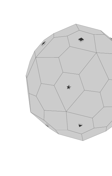
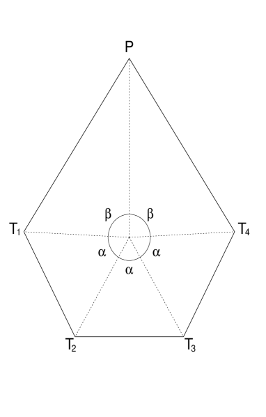
Figure 3: To the left, the pentagonal hexacontahedron shape. Certain faces are marked to indicate resonator positions in a specific proposal —see text— as follows: a square for resonators tuned to the first quadrupole frequency, a triangle for the second, and a star for the monopole. On the right we see the (pentagonal) face of the polyhedron. A few details about it: the confluence point of the dotted lines at the centre is the tangency point of the inscribed sphere to the PHC; the labeled angles have values $\alpha\/$ = 61.863^∘, $\beta\/$ = 87.205^∘; the angles at the $T\/$-vertices are all equal, and their value is 118.1366^∘, while the angle at $P\/$ is 67.4536^∘; the ratio of a long edge (e.g. $PT_{1}$) to a short one (e.g. $T_{1}T_{2}$) is 1.74985, and the radius of the inscribed sphere is twice the long edge of the pentagon, $R\/$ = 2 $PT_{1}$.

Figure 4: Compared line spectrum of a coupled TIGA and a PHC resonator layout in an ideally spherical system. The weakly coupled central frequency in the TIGA is drawn dashed. The frequency pair is 5-fold degenerate for this layout, while the two outer pairs of the PHC are doubly degenerate each, and the inner pair is non-degenerate. Units in abscissas are $\eta^{1/2}\Omega$, and the central value, labeled 0.0, corresponds to $\Omega$.

Based on these facts one may next ask which is a suitable transducer distribution with an axis of pentagonal symmetry. In Figure 2 we give a plot of the eigenvalues (43) as a function of $\alpha\/$, the angular distance of the resonator set from the symmetry axis. Several criteria may be adopted to select a specific choice in view of this graph. An interesting one was proposed by us in reference [Lobo & Serrano 1996] with the following argument. If for ease of mounting, stability, etc., it is desirable to have the detector milled into a close-to-spherical polyhedric shape then polyhedra with axes of pentagonal symmetry must be searched. The number of quasi regular convex polyhedra is of course finite —there actually are only 18 of them [Holden 1977, Har’El 1993]—, and we found a particularly appealing one in the so called pentagonal hexacontahedron (PHC), which we see in Figure 3, left. This is a 60 face polyhedron, whose faces are the identical irregular pentagons of Figure 3, right. The PHC admits an inscribed sphere which is tangent to each face at the central point marked in the Figure. It is clearly to this point that a resonator should be attached so as to simulate an as perfect as possible spherical distribution.

The PHC is considerably spherical: the ratio of its volume to that of the inscribed sphere is 1.057, which quite favourably compares to the value of 1.153 for the ratio of the circumscribed sphere to the TI volume. If we now request that the frequency pairs $\omega_{m\pm}$ be as evenly spaced as possible, compatible with the PHC face orientations, then we must choose $\alpha\/$ = 67.617^∘, whence

$$\omega_{0\pm}=\omega_{12}\,\left(1\pm 0.5756\,\eta^{1/2}\right)\ ,\ \ \ \omega_{1\pm}=\omega_{12}\,\left(1\pm 0.8787\,\eta^{1/2}\right)\ ,\ \ \ \omega_{2\pm}=\omega_{12}\,\left(1\pm 1.0668\,\eta^{1/2}\right)$$ (49)

for instance for $\Omega$ = $\omega_{12}$, the first quadrupole harmonic. In Figure 4 we display this frequency spectrum together with the multiply degenerate TIGA for comparison.

The criterion leading to the PHC proposal is of course not unique, and alternatives can be considered. For example, if the 5 faces of a regular icosahedron are selected for sensor mounting ($\alpha\/$ = 63.45^∘) then a four-fold degenerate pair plus a single non-degenerate pair is obtained; if the resonator parallel is 50^∘ or 22.6^∘ away from the “north pole” then the three frequencies $\omega_{0+}$, $\omega_{1+}$, and $\omega_{2+}$ are equally spaced; etc. The number of choices is virtually infinite if the sphere is not milled into a polyhedric shape [Stevenson 1997, Magalhães et al. 1997].

Let us finally recall that the complete PHC proposal [Lobo & Serrano 1996] was made with the idea of building an as complete as possible spherical GW antenna, which amounts to making it sensitive at the first two quadrupole frequencies and at the first monopole one. This would take advantage of the good sphere cross section at the second quadrupole harmonic [Coccia et al. 1995a], and would enable measuring (or thresholding) eventual monopole GW radiation. Now, the system pattern matrix $\hat{\Lambda}_{a}^{(lm)}(s;\Omega)$ has identical structure for all the harmonics of a given $l\/$ series —see (36) and (39)—, and so too identical criteria for resonator layout design apply to either set of transducers, respectively tuned to $\omega_{12}$ and $\omega_{22}$. The PHC proposal is best described graphically in Figure 3, left: a second set of resonators, tuned to the second quadrupole harmonic $\omega_{22}$ can be placed in an equivalent position in the “southern hemisphere”, and an eleventh resonator tuned to the first monopole frequency $\omega_{10}$ is added at an arbitrary position. It is not difficult to see, by the general methods outlined earlier on in this paper, that cross interaction between these three sets of resonators is only second order in $\eta^{1/2}\/$, therefore weak.

A spherical GW detector with such a set of altogether 11 transducers would be a very complete multi-mode multi-frequency device with an unprecedented capacity as an individual antenna. Amongst other it would practically enable monitoring of coalescing binary chirp signals by means of a rather robust double passage method [Coccia & Fafone 1996], a prospect which was considered so far possible only with broadband long baseline laser interferometers [Dhurandhar, Krolak & Lobo 1989, Krolak, Lobo & Meers 1991], and is almost unthinkable with currently operating cylindrical bars.

6 A calibration signal: hammer stroke

This section is a brief digression from the main streamline of the paper. We propose to assess now the system response to a particular, but useful, calibration signal: a perpendicular hammer stroke.

We first go back to equation (23) and replace $\hat{u}_{a}^{\rm external}(s)$ in its rhs with that corresponding to a hammer stroke, which is easily calculated —cf. appendix A:

$$\hat{u}_{a}^{\rm stroke}(s)=-\sum_{nl}\,\frac{f_{0}}{s^{2}+\omega_{nl}^{2}}\,\left|A_{nl}(R)\right|^{2}\,P_{l}({\bf n}_{a}\!\cdot\!{\bf n}_{0})\ ,\qquad a=1,\ldots,J$$ (50)

where ${\bf n}_{0}$ are the spherical coordinates of the hit point on the sphere, and $f_{0}$ $\equiv$ ${\bf n}_{0}\!\cdot\!{\bf f}_{0}/{\cal M\/}$. Clearly, the hammer stroke excites all of the sphere’s vibration eigenmodes, as it has a completly flat spectrum.

The coupled system resonances are again those calculated in appendix B. The same procedures described in section 4 for a GW excitation can now be pursued to obtain

$$\hat{q}_{a}(s) = \eta^{-1/2}\,(-1)^{J-1}\,\sqrt{\frac{2l+1}{4\pi}}\,f_{0}\,\left|A_{nl}(R)\right|\,\times$$ (51)

$$\times \sum_{b=1}^{J}\,\left\{\sum_{\zeta_{c}\neq 0}\,\frac{1}{2}\left[\left(s^{2}+\omega_{c+}^{2}\right)^{-1}-\left(s^{2}+\omega_{c-}^{2}\right)^{-1}\right]\,\frac{v_{a}^{(c)}v_{b}^{(c)*}}{\zeta_{c}}\right\}\,P_{l}({\bf n}_{b}\!\cdot\!{\bf n}_{0})+O(0)\ ,\qquad a=1\,\ldots,J$$

when the system is tuned to the $nl\/$-th spheroidal harmonic, i.e., $\Omega$ = $\omega_{nl}$. It is immediately seen from here that the system response to this signal when the resonators are tuned to a monopole frequency is given by

$$\hat{q}_{a}(s)=\eta^{-1/2}\,(-1)^{J-1}\,\frac{f_{0}}{\sqrt{4\pi J}}\,\left|A_{n0}(R)\right|\,\frac{1}{2}\left[\left(s^{2}+\omega_{+}^{2}\right)^{-1}-\left(s^{2}+\omega_{-}^{2}\right)^{-1}\right]\ ,\qquad\Omega=\omega_{n0}$$ (52)

an expression which holds for all $a\/$, and is independent of either the resonator layout or the hit point, which in particular prevents any determination of the latter, as obviously expected. The frequencies $\omega_{\pm}$ are those of (35), and we find here again a global factor $J^{-1/2}$, as also expected.

We consider next the situation when quadrupole tuning is implemented, $\Omega$ = $\omega_{n2}$. We shall however do so only for the PHC and TIGA configurations, as more general considerations are not quite as interesting at this point.

Figure 5: Simulated response of a PHC to a hammer stroke: the time series and their respective spectra, both for direct resonator readouts and mode channels. Note that while the former are not simple beats, the latter are.

6.1 PHC and TIGA response to a hammer stroke

Expanding equation 51 by substitution of the eigenvalues $\zeta_{m}\/$ and eigenvectors $v^{(m)}_{a}\/$ of the PHC, one readily finds that the system response is given by

$$\hat{q}_{a}(s)=\eta^{-1/2}\,f_{0}\,\sqrt{\frac{4\pi}{5}}\,\left|A_{n2}(R)\right|\,\sum_{m=-2}^{2}\,\frac{1}{2}\left[\left(s^{2}+\omega_{m+}^{2}\right)^{-1}-\left(s^{2}+\omega_{m-}^{2}\right)^{-1}\right]\,\zeta_{m}^{-1}\,Y_{2m}({\bf n}_{a})\,Y_{2m}^{*}({\bf n}_{0})\ ,\qquad a=1,\ldots,5$$ (53)

and the mode channels by

$$\hat{y}^{(m)}(s)=\eta^{-1/2}\,f_{0}\,\left|A_{n2}(R)\right|\frac{1}{2}\left[\left(s^{2}+\omega_{m+}^{2}\right)^{-1}-\left(s^{2}+\omega_{m-}^{2}\right)^{-1}\right]\,Y_{2m}^{*}({\bf n}_{0})\ ,\ \ m=-2,\ldots,2$$ (54)

These equations indicate that the system response $q_{a}(t)$ is a superposition of three different beats, while the mode channels are single beats each, but with differing modulation frequencies. This is represented graphically in Figure 5, where we see the result of a numerical simulation of the PHC response to a hammer stroke, delivered to the solid at a given location. The readouts $q_{a}(t)$ are somewhat complex time series, whose frequency spectrum shows three pairs of peaks —in fact, the lines in the ideal spectrum of Figure 4. The mode channels on the other hand are pure beats, whose spectra consist of the individually separate pairs of the just mentioned peaks.

The response of the TIGA layout to a hammer stroke has been described in detail by Merkowitz and Johnson —see e.g. reference [Merkowitz & Johnson 1997]. Our formalism does of course recover the results obtained by those authors; in the notation of this paper, we have

$$\hat{q}_{a}(s) = -\eta^{-1/2}\,\frac{5}{\sqrt{24\pi}}\,f_{0}\,\left|A_{n2}(R)\right|\,\frac{1}{2}\left[\left(s^{2}+\omega_{+}^{2}\right)^{-1}-\left(s^{2}+\omega_{-}^{2}\right)^{-1}\right]\,P_{2}({\bf n}_{a}\!\cdot\!{\bf n}_{0})\ ,\qquad{\sl TIGA}$$ (55)

$$\hat{y}^{(m)}(s) = -\eta^{-1/2}\,f_{0}\,\left|A_{n2}(R)\right|\frac{1}{2}\left[\left(s^{2}+\omega_{+}^{2}\right)^{-1}-\left(s^{2}+\omega_{-}^{2}\right)^{-1}\right]\,Y_{2m}^{*}({\bf n}_{0})\ ,\ \ m=-2,\ldots,2$$ (56)

for the system response and the mode channels, respectively, where

$$\omega_{\pm}^{2}=\omega_{n2}^{2}\,\left(1\pm\sqrt{\frac{3}{2\pi}}\,\left|A_{n2}(R)\right|\eta^{1/2}\right)+O(\eta)\ ,\qquad a=1,\ldots,6$$ (57)

are the five-fold degenerate frequency pairs corresponding to the TIGA distribution. Comparison of the mode channels shows that they are identical for PHC and TIGA, except that the former come at different frequencies depending on the index $m\/$. One might perhaps say that the PHC gives rise to a sort of “Zeeman splitting” of the TIGA degenerate frequencies, which can be attributed to an axial symmetry breaking of that resonator distribution: the PHC mode channels partly split up the otherwise degenerate multiplet into its components.

7 Symmetry defects

So far we have made the assumption that the sphere is perfectly symmetric, that the resonators are identical, that their locations on the sphere’s surface are ideally accurate, etc. This is of course unrealistic. So we propose to address now how such departures from ideality affect the system behaviour. As we shall see, the system is rather robust, in a sense to be made precise shortly, against a number of small defects.

In order to quantitatively assess ideality failures we shall adopt a philosophy which is naturally suggested by the results already obtained in an ideal system. It is as follows.

As we have seen in previous sections, the solution to the general equations (23) must be given as a perturbative series expansion in ascending powers of the small quantity $\eta^{1/2}$. This is clearly a fact not related to the system’s symmetries, so it will survive symmetry breakings. It is therefore appropriate to parametrize deviations from ideality in terms of suitable powers of $\eta^{1/2}$, in order to address them consistently with the order of accuracy of the series solution to the equations of motion. An example will better illustrate the situation.

In a perfectly ideal spherical detector the system frequencies are given by equations (31). Now, if a small departure from e.g. spherical symmetry is present in the system then we expect that a correspondingly small correction to those equations will be required. Which specific correction to the formula will actually happen can be qualitatively assessed by a consistency argument: if symmetry defects are of order $\eta^{1/2}$ then equations (31) will be significantly altered in their $\eta^{1/2}$ terms; if on the other hand such defects are of order $\eta\/$ or smaller then any modifications to equations (31) will be swallowed into the $O(0)$ terms, and the more important $\eta^{1/2}$ terms will remain unaffected by the symmetry failure. We will say in the latter case that the system is robust to that ideality breaking.

More generally, this argument can be extended to see that the only system defects standing a chance to have any influences on lowest order ideal system behaviour are defects of order $\eta^{1/2}$ relative to an ideal configuration. Defects of such order are however not necessarily guaranteed to be significant, and a specific analysis is required for each specific parameter in order to see whether or not the system response is robust against the considered parameter deviations.

We therefore proceed as follows. Let $P\/$ be one of the system parameters, e.g. a sphere frequency, or a resonator mass or location, etc. Let $P_{\rm ideal}$ be the numerical value this parameter has in an ideal detector, and let $P_{\rm real}$ be its value in the real case. These two will be assumed to differ by terms of order $\eta^{1/2}$, or

$$P_{\rm real}=P_{\rm ideal}\,(1+p\,\eta^{1/2})$$ (58)

For a given system, $p\/$ is readily determined adopting (58) as the definition of $P_{\rm real}$, once a suitable hypothesis has been made as to which is the value of $P_{\rm ideal}$. In order for the following procedure to make sensible sense it is clearly required that $p\/$ be of order 1 or, at least, appreciably larger than $\eta^{1/2}$. Should $p\/$ thus calculated from (58) happen to be too small, i.e., of order $\eta^{1/2}$ itself or smaller, then the system will be considered robust as regards the affected parameter.

We now apply this criterion to various departures from ideality.

7.1 The suspended sphere

An earth based observatory obviously requires a suspension mechanism for the large sphere. If a nodal point suspension is e.g. selected then a diametral bore has to be drilled across the sphere [Merkowitz 1995]. The most immediate consequence of this is that spherical symmetry is broken, what in turn results in degeneracy lifting of the free spectral frequencies $\omega_{nl}\/$, which now split up into multiplets $\omega_{nlm}\/$ ($m\/$ = $-l\/$,…,$l\/$). The resonators’ frequency $\Omega$ cannot therefore be matched to the frequency $\omega_{n_{0}l_{0}}$, but at most to one of the $\omega_{n_{0}l_{0}m}\/$’s. In this subsection we keep the hypothesis that all the resonators are identical —we shall relax it later—, and assume that $\Omega$ falls within the span of the multiplet of the $\omega_{n_{0}l_{0}m}\/$’s. Then we write

$$\omega_{n_{0}l_{0}m}^{2}=\Omega^{2}\,(1+p_{m}\,\eta^{1/2})\ ,\qquad m=-l_{0},\ldots,l_{0}$$ (59)

We now search for the coupled frequencies, i.e., the roots of equation (100). The kernel matrix $\hat{K}_{ab}(s)$ is however no longer given by (24), due the removed degeneracy of $\omega_{nl}\/$, and we must stick to its general expression (89), or

$$\hat{K}_{ab}(s)=\sum_{nlm}\,\frac{\Omega_{b}^{2}}{s^{2}+\omega_{nlm}^{2}}\,\left|A_{nl}(R)\right|^{2}\,\frac{2l+1}{4\pi}\,Y_{lm}^{*}({\bf n}_{a})\,Y_{lm}({\bf n}_{b})\equiv\sum_{nlm}\,\frac{\Omega_{b}^{2}}{s^{2}+\omega_{nlm}^{2}}\,\chi_{ab}^{(nlm)}$$ (60)

Following the steps of appendix A we now seek the roots of the equation

$$\det\,\left[\delta_{ab}+\eta\,\sum_{m=-l_{0}}^{l_{0}}\,\frac{\Omega^{2}s^{2}}{(s^{2}+\Omega^{2})(s^{2}+\omega_{n_{0}l_{0}m}^{2})}\,\chi_{ab}^{(n_{0}l_{0}m)}+\eta\,\sum_{nl\neq n_{0}l_{0},m}\,\frac{\Omega^{2}s^{2}}{(s^{2}+\Omega^{2})(s^{2}+\omega_{nlm}^{2})}\,\chi_{ab}^{(nlm)}\right]=0$$ (61)

Since $\Omega$ relates to $\omega_{n_{0}l_{0}m}\/$ through equation (59) we see that the roots of (61) fall again into either of the two categories (103)-(104)(see Appendix B), i.e., roots close to $\pm i\Omega$ and roots close to $\pm i\omega_{nlm}\/$ ($nl\/$ $\neq$ $n_{0}l_{0}$). We shall exclusively concentrate on the former now. Direct substitution of the series (103) into (61) yields the following equation for the coefficient $\chi_{\frac{1}{2}}$:

$$\det\left[\delta_{ab}-\frac{1}{\chi_{\frac{1}{2}}}\,\sum_{m=-l_{0}}^{l_{0}}\,\frac{\chi_{ab}^{(n_{0}l_{0}m)}}{\chi_{\frac{1}{2}}-p_{m}}\right]=0$$ (62)

This is a variation of (105), to which it reduces when $p_{m}\/$ = 0, i.e., when there is full degeneracy.

The solutions to (62) no longer come in symmetric pairs, like (31). Rather, there are 2$l_{0}$+1+$J\/$ of them, with a maximum number of 2(2$l_{0}$+1) non-identically zero roots if $J\/$ $\geq$ 2$l_{0}$+1. For example, if we choose to select the resonators’ frequency close to a quadrupole multiplet ($l_{0}$ = 2) then (62) has at most 5+$J\/$ non-null roots, with a maximum ten no matter how many resonators in excess of 5 we attach to the sphere. Modes associated to null roots of (62) can be seen to be weakly coupled, just like in a free sphere, i.e., their amplitudes are smaller than those of the strongly coupled ones by factors of order $\eta^{1/2}$.

In order to assess the reliability of this method we have applied it to see what are its predictions for a real system. To this end, data taken with the TIGA prototype at LSU were used to confront with. The TIGA was drilled and suspended from its centre, so its first quadrupole frequency split up into a multiplet of five frequencies. Their reportedly measured values are

$$\omega_{120}=3249\ {\rm Hz}\ ,\ \ \omega_{121}=3238\ {\rm Hz}\ ,\ \ \omega_{12\,-1}=3236\ {\rm Hz}\ ,\ \ \omega_{122}=3224\ {\rm Hz}\ ,\ \ \omega_{12\,-2}=3223\ {\rm Hz}\ ,\ \$$ (63)

All 6 resonators were equal, and had the following characteristic frequency and mass, respectively:

$$\Omega=3241\ {\rm Hz}\ ,\qquad\eta=\frac{1}{1762.45}$$ (64)

Substituting these values into (59) it is seen that

$$p_{0}=0.2075\ ,\ \ p_{1}=-0.0777\ ,\ \ p_{-1}=-0.1036\ ,\ \ p_{2}=-0.4393\ ,\ \ p_{-2}=-0.4650$$ (65)

Table 1: Numerical values of measured and theoretically predicted frequencies (in Hz) for the TIGA prototype with varying number of resonators. Percent differences are also shown. The calculated values of the tuning and free multiplet frequencies are taken by definition equal to the measured ones, and quoted in brackets. In square brackets the frequency of the weakly coupled sixth mode in the full, 6 resonator TIGA layout. These data are plotted in Figure 6.

Item	Measured	Calculated	% difference	Item	Measured	Calculated	% difference
Tuning	3241	(3241)	(0.00)	4 resonators	3159	3155	$-0.12$
Free multiplet	3223	(3223)	(0.00)		3160	3156	$-0.11$
	3224	(3224)	(0.00)		3168	3165	$-0.12$
	3236	(3236)	(0.00)		3199	3198	$-0.05$
	3238	(3238)	(0.00)		3236	3236	$0.00$
	3249	(3249)	(0.00)		3285	3286	$0.03$
1 resonator	3167	3164	$-0.08$		3310	3310	$0.00$
	3223	3223	$0.00$		3311	3311	$0.00$
	3236	3235	$-0.02$		3319	3319	$0.00$
	3238	3237	$-0.02$	5 resonators	3152	3154	$0.08$
	3245	3245	$0.00$		3160	3156	$-0.14$
	3305	3307	$0.06$		3163	3162	$-0.03$
2 resonators	3160	3156	$-0.13$		3169	3167	$-0.08$
	3177	3175	$-0.07$		3209	3208	$-0.02$
	3233	3233	$0.00$		3268	3271	$0.10$
	3236	3236	$0.00$		3304	3310	$0.17$
	3240	3240	$0.00$		3310	3311	$0.03$
	3302	3303	$0.03$		3313	3316	$0.10$
	3311	3311	$0.00$		3319	3321	$0.06$
3 resonators	3160	3155	$-0.15$	6 resonators	3151	3154	$0.11$
	3160	3156	$-0.13$		3156	3155	$-0.03$
	3191	3190	$-0.02$		3162	3162	$0.00$
	3236	3235	$-0.02$		3167	3162	$-0.14$
	3236	3236	$0.00$		3170	3168	$-0.07$
	3297	3299	$0.08$		[3239]	[3241]	[0.06]
	3310	3311	$0.02$		3302	3309	$0.23$
	3311	3311	$0.00$		3308	3310	$0.06$
					3312	3316	$0.12$
					3316	3317	$0.02$
					3319	3322	$0.10$

Equation (62) can now be readily solved once the resonator positions are fed into the matrices $\chi_{ab}^{(12m)}$. Such positions correspond to the pentagonal faces of a truncated icosahedron. Merkowitz [Merkowitz 1995] gives a complete account of all the measured system frequencies as resonators are progressively attached to the selected faces, beginning with one and ending with six. In Figure 6 we present a graphical display of the experimentally reported frequencies along with those calculated theoretically by solving equation (62). In Table 1 we give the numerical values. As can be seen, coincidence between our theoretical predictions and the experimental data is remarkable: the worst error is 0.2%, while for the most part it is below 0.1%. Thus discrepancies between our theoretical predictions and experiment are of order $\eta$, as indeed expected —see (64). In addition, it is also reported in reference [Merkowitz & Johnson 1997] that the 11-th, weakly coupled mode of the TIGA (enclosed in square brackets in Table 1) has a practically zero amplitude, again in excellent agreement with our general theoretical predictions about modes beyond the tenth —see paragraph after equation (62).

Figure 6: The frequency spectrum of the TIGA distribution as resonators are progressively added from none to 6. Continuous lines correspond to measured values, and dashed lines correspond to their $\eta^{1/2}$ theoretical estimates with equation (62).

This is an encouraging result which motivated us to try a better fit by estimating the next order corrections, i.e., $\chi_{1}$ of (103). As it turned out, however, matching between theory and experiment did not consistently improve. This is not really that surprising, though, as M&J explicitly state [Merkowitz & Johnson 1997] that control of the general experimental conditions in which data were obtained had a certain degree of tolerance, and they actually show satisfaction that $\sim$1% coincidence between theory and measurement is comfortably accomplished. But 1% is two orders of magnitude larger than $\eta\/$ —cf. equation (64)—, so failure to refine our frequency estimates to order $\eta\/$ is again fully consistent with the accuracy of available real data.

A word on a technical issue is in order. Merkowitz and Johnson’s equations for the TIGA [Johnson & Merkowitz 1993, Merkowitz & Johnson 1995] are identical to ours to lowest order in $\eta\/$. Remarkably, though, their reported theoretical estimates of the system frequencies are not quite as accurate as ours [Merkowitz & Johnson 1997]. The reason for this is probably the following: in M&J’s model these frequencies appear within an algebraic system of 5+$J\/$ linear equations with as many unknowns which has to be solved; in our model the algebraic system has only $J\/$ equations and unknowns, actually equations (23). This is a very appreciable difference for the range of values of $J\/$ under consideration. While the roots for the frequencies can be seen to mathematically coincide in both approaches, in actual practice these roots are estimated, generally by means of computer programmes. It is here that problems most likely arise, for the numerical reliability of an algorithm to solve matrix equations normally decreases as the rank of the matrix increases. The significant algebraic simplification of our model’s equations should therefore be considered one of real practical value.

7.2 Other mismatched parameters

We now assess the system sensitivity to small mismatches in resonators’ masses, locations and frequencies.

7.2.1 Resonator mass mismatches

If the masses are slightly non-equal then we can write

$$M_{a}=\eta{\cal M}\,(1+\mu_{a}\,\eta^{1/2})\ ,\qquad a=1,\ldots,J$$ (66)

where $\eta\/$ can be defined e.g. as the ratio of the average resonator mass to the sphere’s mass. It is immediately obvious from equation (66) that mass non-uniformities of the resonators only affect our equations in second order, since resonator mass non-uniformities result, as we see, in corrections of order $\eta^{1/2}$ to $\eta^{1/2}$ itself, which is the very parameter of the perturbative expansions. The system is thus clearly robust to mismatches in the resonator masses of the type (66).

7.2.2 Errors in resonator locations

The same happens if the locations of the resonators have tolerances relative to a pre-selected distribution. For let ${\bf n}_{a}\/$ be a set of resonator locations, for example the TIGA or the PHC positions, and let ${\bf n^{\prime}}_{a}\/$ be the real ones, close to the former:

$${\bf n^{\prime}}_{a}={\bf n}_{a}+{\bf v}_{a}\,\eta^{1/2}\ ,\qquad a=1,\ldots,J$$ (67)

The values ${\bf n}_{a}$ determine the eigenvalues $\zeta_{a}\/$ in equation (31), and also they appear as arguments to the spherical harmonics in the system response functions of sections 4–6. It follows from (67) by continuity arguments that

$$Y_{lm}({\bf n^{\prime}}_{a}) = Y_{lm}({\bf n}_{a})+O(\eta^{1/2})$$ (68)

$$\zeta^{\prime}_{a} = \zeta_{a}+O(\eta^{1/2})$$ (69)

Inspection of the equations of sections 4–6 shows that both $\zeta_{a}\/$ and $Y_{lm}({\bf n}_{a})$ always appear within lowest order terms, and hence that corrections to them of the type (68)-(69) will affect those terms in second order again. We thus conclude that the system is also robust to small misalignments of the resonators relative to pre-established positions.

7.2.3 Resonator frequency mistunings

The resonator frequencies may also differ amongst them, so let

$$\Omega_{a}=\Omega\,(1+\rho_{a}\,\eta^{1/2})\ ,\qquad a=1,\ldots,J$$ (70)

To assess the consequences of this, however, we must go back to equation (100) and see what the coefficients in its series solutions of the type (103) are. The procedure is very similar to that of section 7.1, and will not be repeated here; the lowest order coefficient $\chi_{\frac{1}{2}}$ is seen to satisfy the algebraic equation

$$\det\left[\delta_{ab}-\frac{1}{\chi_{\frac{1}{2}}}\,\sum_{c=0}^{J}\,\frac{\chi_{ac}^{(n_{0}l_{0})}\,\delta_{cb}}{\chi_{\frac{1}{2}}-\rho_{c}}\right]=0$$ (71)

which reduces to (105) when all the $\rho\/$’s vanish, as expected. This appears to potentially have significant effects on our results to lowest order in $\eta^{1/2}$, but a more careful consideration of the facts shows that it is probably unrealistic to think of such large tolerances in resonator manufacturing as implied by equation (70) in the first place. In the TIGA experiment, for example [Merkowitz 1995], an error of order $\eta^{1/2}$ would amount to around 50 Hz of mistuning between resonators, an absurd figure by all means. In a full scale sphere ($\sim$40 tons, $\sim$3 metres in diameter, $\sim$800 Hz fundamental quadrupole frequency, $\eta\/$ $\sim$ 10^-5) the same error would amount to between 5 Hz and 10 Hz in resonator mistunings for the lowest frequency. This is probably excessive for a capacitive transducer, but may be realistic for an inductive one. With this exception, it is thus more appropriate to consider that resonator mistunings are at least of order $\eta\/$. If this is the case, though, we see once more that the system is quite insensitive to such mistunings.

Summing up the results of this section, we can say that the resonator system dynamics is quite robust to small (of order $\eta^{1/2}$) changes in its various parameters. The important exception is of course the effect of suspension drillings, which do result in significant changes relative to the ideally perfect device, but which can be relatively easily calculated. This theoretical picture is fully supported by experiment, as robustness in the parameters here considered has been reported in reference [Merkowitz & Johnson 1997].

8 Conclusions

A spherical GW antenna is a natural multimode device with very rich potential capabilities to detect GWs on earth. But such detector is not just a bare sphere, it requires a set of motion sensors to be practically useful. It appears that transducers of the resonant type are the best suited ones for an efficient performance of the detector. Resonators however significantly interact with the sphere, and they affect in particular its frequency spectrum and vibration modes in a specific fashion, which has to be properly understood before reliable conclusions can be drawn from the system readout.

The main objective of this paper has been the construction and development of an elaborate theoretical model to describe the joint dynamics of a solid elastic sphere and a set of radial motion resonators attached to its surface at arbitrary locations, with the purpose to make predictions of the system characteristics and response, in principle with arbitrary mathematical precision.

We have shown that the solutions to our equations of motion are expressible as an ascending series in powers of the small “coupling constant” $\eta\/$, the ratio of the average resonator mass to the mass of the large sphere. The lowest order approximation corresponds to terms of order $\eta^{1/2}$ and, to this order, we recover, and widely generalise, other authors’ results [Merkowitz & Johnson 1997, Stevenson 1997, Magalhães et al. 1997], obtained by them on the basis of certain simplifying assumptions. This has in particular enabled us to assess the system response for arbitrary resonator layouts, and to search the equations for configurations other than the highly symmetric TIGA. This search has led us to make a specific proposal, the PHC, which is based on a pentagonally symmetric set of 5 rather than 6 resonators per quadruopole mode sensed. The PHC distribution has the very interesting property that mode channels can be constructed from the resonators’ readouts, much in the same way as in the TIGA [Merkowitz & Johnson 1995]. In the PHC however a new and distinctive characteristic is present: different wave amplitudes selectively couple to different detector modes having different frequencies, so that the antenna’s mode channels come at different rather than equal frequencies. The PHC philosophy can be extended to make a multifrequency system by using resonators tuned to the first two quadrupole harmonics of the sphere and to the first monopole, an altogether 11 transducer set [Lobo & Serrano 1996].

The assessment of symmetry failure effects, as well as other parameter departures form ideality, has also interested us here. This is seen to receive a particularly clear treatment in our general scheme: the theory transparently shows that the system is robust against relative disturbances of order $\eta\/$ or smaller in any system parameters, and provides a systematic procedure to assess larger tolerances —up to order $\eta^{1/2}$. The system is shown to still be robust to tolerances of this order in some of its parameters, whilst it is not to others. Included in the latter group is the effect of spherical symmetry breaking due to system suspension in the laboratory, which causes degeneracy lifting of the sphere’s eigenfrequencies, now split up into multiplets. By using our algorithms we have succeeded in numerically reproducing the reportedly measured frequencies of the LSU prototype antenna [Merkowitz 1995] with a fully satisfactory precision of four decimal places. The experimentally reported robustness of the system to resonator mislocations [Merkowitz & Johnson 1997] is also in full agreement with our theoretical predictions.

The perturbative approach we have adopted is naturally open to refined analysis of the system response in higher orders in $\eta\/$. For example, we can systematically address the weaker coupling of non-quadrupole modes. It appears however that such refinements will be largely masked by noise in a real system, as shown by Merkowitz and Johnson [Merkowitz & Johnson 1998], and this must therefore be considered first. So our next step is to include noise in the model and see its effect. Stevenson [Stevenson 1997] has already made some progress in this direction, and partly assessed the characteristics of TIGA and PHC, but more needs to be done since not too high signal-to-noise ratios should realistically be be considered in an actual GW detector. In particular, the discovery of mode channels also for the PHC distribution opens the possibility of analysis of noise correlations and dependencies, as well as the errors in GW parameter estimation. These are natural extensions of this research, and some of them are currently underway [Merkowitz, Lobo & Serrano 1999].

Appendix A Green functions for the multiple resonator system

The density of forces in he rhs of equation (2) happens to be of the separable type

$${\bf f}({\bf x},t)=\sum_{\alpha}\,{\bf f}^{(\alpha)}({\bf x})\,g^{(\alpha)}(t)$$ (72)

where $\alpha\/$ is a suitable label. We recall from reference [Lobo 1995] that, in such circumstances, a formal solution can be written down for equation (2) in terms of a Green function integral, whereby the following orthogonal series expansion obtains:

$${\bf u}({\bf x},t)=\sum_{\alpha}\sum_{N}\,\omega_{N}^{-1}\,f_{N}^{(\alpha)}\,{\bf u}_{N}({\bf x})\,g_{N}^{(\alpha)}(t)$$ (73)

where

$$f_{N}^{(\alpha)} \equiv \frac{1}{\cal M}\,\int_{\rm Sphere}{\bf u}_{N}^{*}({\bf x})\cdot{\bf f}^{(\alpha)}({\bf x})\,d^{3}x$$ (74)

$$g_{N}^{(\alpha)}(t) \equiv \int_{0}^{t}g^{(\alpha)}(t^{\prime})\,\sin\omega_{N}(t-t^{\prime})\,dt^{\prime}$$ (75)

Here, $\omega_{N}\/$ and ${\bf u}_{N}({\bf x})$ are the eigenfrequencies and associated normalised wavefunctions of the free sphere. Also, $N\/$ is an abbreviation for a multiple index $\{nlm\}$. The generic index $\alpha$ is a label for the different pieces of interaction happening in the system. We quote the result of the calculations of the terms required in this paper:

$$f_{{\rm resonators,}N}^{(a)} = \frac{M_{a}}{\cal M}\,\Omega_{a}^{2}\,\,\left[{\bf n}_{a}\!\cdot\!{\bf u}_{N}^{*}({\bf x}_{a})\right]\ ,\qquad a=1,\ldots,J$$ (76)

$$f_{{\rm GW,}N}^{(l^{\prime}m^{\prime})} = a_{nl}\,\delta_{ll^{\prime}}\,\delta_{mm^{\prime}}\ \ ,\qquad N\equiv\{nlm\}\ ,\ \ l^{\prime}=0,2\ ,\ \ m^{\prime}=-l^{\prime},\ldots,l^{\prime}$$ (77)

$$f_{{\rm stroke,}N} = {\cal M}^{-1}\,{\bf f}_{0}\!\cdot\!{\bf u}_{N}^{*}({\bf x}_{0})$$ (78)

where the coefficients $a_{nl}\/$ in (77) are overlapping integrals of the type (74) , and

$$g_{{\rm resonators,}N}^{(a)}(t) = \int_{0}^{t}\left[z_{a}(t^{\prime})-u_{a}(t)\right]\,\sin\omega_{N}(t-t^{\prime})\,dt^{\prime}\ \ ,\qquad a=1,\ldots,J$$ (79)

$$g_{{\rm GW,}N}^{(lm)}(t) = \int_{0}^{t}g^{(lm)}(t^{\prime})\,\sin\omega_{N}(t-t^{\prime})\,dt^{\prime}$$ (80)

$$g_{{\rm stroke,}N}(t) = \sin\omega_{N}t$$ (81)

If this is replaced into (2) one readily finds

$${\bf u}({\bf x},t)=\sum_{N}\,\omega_{N}^{-1}\,{\bf u}_{N}({\bf x})\,\left\{\sum_{b=1}^{J}\,\frac{M_{b}}{\cal M}\,\Omega_{b}^{2}\,\left[{\bf n}_{b}\!\cdot\!{\bf u}_{N}^{*}({\bf x}_{b})\right]\,g_{{\rm resonators,}N}^{(b)}(t)+\sum_{\alpha}f_{{\rm external,}N}^{(\alpha)}\,g_{{\rm external,}N}^{(\alpha)}(t)\right\}$$ (82)

where the label “external” explicitly refers to agents acting upon the system from outside; two kinds of such external actions are considered in this article: those due to GWs and those due to a calibration hammer stroke. Specifying x = ${\bf x}_{a}\/$ in and multiply by ${\bf n}_{a}\/$ above, the following is readily found:

$$u_{a}(t) = u_{a}^{\rm external}(t)+\sum_{b=1}^{J}\,\eta_{b}\,\int_{0}^{t}K_{ab}(t-t^{\prime})\,\left[\,z_{b}(t^{\prime})-u_{b}(t^{\prime})\right]\,dt^{\prime}$$ (83)

$$\ddot{z}_{a}(t) = \xi_{a}^{\rm external}(t)-\Omega_{a}^{2}\,\left[\,z_{a}(t)-u_{a}(t)\right]\ ,\qquad a=1,\ldots,J$$ (84)

where $\eta_{b}$ $\equiv$ $M_{b}/{\cal M}$, $u_{a}^{\rm external}(t)$ $\equiv$  ${\bf n}_{a}\!\cdot\!{\bf u}^{\rm external}({\bf x}_{a},t)$,

$${\bf u}^{\rm external}({\bf x},t)=\sum_{\alpha}\sum_{N}\,\omega_{N}^{-1}\,f_{{\rm external,}N}^{(\alpha)}\,{\bf u}_{N}({\bf x})\,g_{{\rm external,}N}^{(\alpha)}(t)$$ (85)

and

$$K_{ab}(t)\equiv\Omega_{b}^{2}\,\sum_{N}\,\omega_{N}^{-1}\,\left[{\bf n}_{b}\!\cdot\!{\bf u}_{N}^{*}({\bf x}_{b})\right]\left[{\bf n}_{a}\!\cdot\!{\bf u}_{N}({\bf x}_{a})\right]\,\sin\omega_{N}t$$ (86)

The following bare sphere responses to GWs and hammer strokes (equations (1) and (10), respectively) can be calculated by direct substitution. We present here the results as Laplace transform domain functions, which are the useful ones for our purposes:

$$\hat{u}_{a}^{\rm GW}(s) = \sum_{\stackrel{{\scriptstyle\scriptstyle l=0\ {\rm and}\ 2}}{{m=-l,...,l}}}\,\left(\sum_{n=1}^{\infty}\,\frac{a_{nl}\,A_{nl}(R)}{s^{2}+\omega_{nl}^{2}}\right)\,Y_{lm}({\bf n}_{a})\,\hat{g}^{(lm)}(s)\ ,\qquad a=1,\ldots,J$$ (87)

$$\hat{u}_{a}^{\rm stroke}(s) = -\sum_{nl}\,\frac{f_{0}}{s^{2}+\omega_{nl}^{2}}\,\left|A_{nl}(R)\right|^{2}\,P_{l}({\bf n}_{a}\!\cdot\!{\bf n}_{0})\ ,\qquad a=1,\ldots,J$$ (88)

where $Y_{lm}\/$ are spherical harmonics and $P_{l}\/$ Legendre polynomials [Edmonds 1960]. The calculation of the Laplace transform of the kernel matrix (86) is likewise immediate:

$$\hat{K}_{ab}(s)=\sum_{N}\,\frac{\Omega_{b}^{2}}{s^{2}+\omega_{N}^{2}}\,\left[{\bf n}_{b}\!\cdot\!{\bf u}_{N}^{*}({\bf x}_{b})\right]\left[{\bf n}_{a}\!\cdot\!{\bf u}_{N}({\bf x}_{a})\right]$$ (89)

Given that (see [Lobo 1995] for full details)

$${\bf u}_{nlm}({\bf x})=A_{nl}(r)\,Y_{lm}(\theta,\varphi)\,{\bf n}-B_{nl}(r)\,i{\bf n}\!\times\!{\bf L}Y_{lm}(\theta,\varphi)$$ (90)

and that the spheroidal frequencies $\omega_{nl}\/$ are 2$l\/$+1–fold degenerate, (89) can be easily summed over the degeneracy index $m\/$, to obtain

$$\hat{K}_{ab}(s)=\sum_{nl}\,\frac{\Omega_{b}^{2}}{s^{2}+\omega_{nl}^{2}}\,\left|A_{nl}(R)\right|^{2}\,\left[\sum_{m=-l}^{l}\,Y_{lm}^{*}({\bf n}_{b})\,Y_{lm}({\bf n}_{a})\right]$$ (91)

or, equivalently,

$$\hat{K}_{ab}(s)=\sum_{nl}\,\frac{\Omega_{b}^{2}}{s^{2}+\omega_{nl}^{2}}\,\left|A_{nl}(R)\right|^{2}\,\frac{2l+1}{4\pi}\,P_{l}({\bf n}_{a}\!\cdot\!{\bf n}_{b})$$ (92)

where use has been made of the summation formula for the spherical harmonics [Edmonds 1960]

$$\sum_{m=-l}^{l}\,Y_{lm}^{*}({\bf n}_{b})\,Y_{lm}({\bf n}_{a})=\frac{2l+1}{4\pi}\,P_{l}({\bf n}_{a}\!\cdot\!{\bf n}_{b})$$ (93)

and where $P_{l}\/$ is a Legendre polynomial:

$$P_{l}(z)=\frac{1}{2^{l}\,l!}\,\frac{d^{l}}{dz^{l}}\,(z^{2}-1)^{l}$$ (94)

Appendix B System response algebra

From equation (27), i.e.,

$$\sum_{b=1}^{J}\,\left[\delta_{ab}+\eta\,\sum_{nl}\,\frac{\Omega^{2}s^{2}}{(s^{2}+\Omega^{2})(s^{2}+\omega_{nl}^{2})}\,\chi_{ab}^{(nl)}\right]\,\hat{q}_{b}(s)=-\frac{s^{2}}{s^{2}+\Omega^{2}}\,\hat{u}_{a}^{\rm GW}(s)+\frac{\hat{\xi}_{a}^{\rm GW}(s)}{s^{2}+\Omega^{2}}\ ,\qquad(\Omega=\omega_{n_{0}l_{0}})$$ (95)

we must first isolate $\hat{q}_{b}(s)$, then find inverse Laplace transforms to revert to time domain quantities. Substituting the values of $\hat{u}_{a}^{\rm GW}(s)$ and $\hat{\xi}_{a}^{\rm GW}(s)$ from (87) and (28) into (95) we find

$$\hat{q}_{a}(s)=\sum_{\mbox{\scriptsize$\begin{array}[]{c}l=0\ \mbox{and}\ 2\\ m=-l,...,l\end{array}$}}\hat{\Phi}_{a}^{(lm)}(s)\,\hat{g}^{(lm)}(s)\ ,\qquad a=1,\ldots,J$$ (96)

where

$$\hat{\Phi}_{a}^{(lm)}(s)=-\frac{s^{2}}{s^{2}+\Omega^{2}}\,\left(-\frac{R}{s^{2}}+\sum_{n=1}^{\infty}\,\frac{a_{nl}\,A_{nl}(R)}{s^{2}+\omega_{nl}^{2}}\right)\,\sum_{b=1}^{J}\,\left[\delta_{ab}+\eta\,\sum_{nl}\,\frac{\Omega^{2}s^{2}}{(s^{2}+\Omega^{2})(s^{2}+\omega_{nl})^{2}}\,\chi_{ab}^{(nl)}\right]^{-1}\,Y_{lm}({\bf n}_{b})$$ (97)

Now, using the convolution theorem of Laplace transforms, we see that the time domain version of equation (96) is

$$q_{a}(t)=\sum_{lm}\,\int_{0}^{t}\,\Phi_{a}^{(lm)}(t-t^{\prime})\,g^{(lm)}(t^{\prime})\,dt^{\prime}\ ,\qquad a=1,\ldots,J$$ (98)

where $\Phi_{a}^{(lm)}(t)$ is the inverse Laplace transform of (97). The inverse Laplace transform of $\hat{\Phi}_{a}^{(lm)}(s)$ can be expediently calculated by the residue theorem through the formula [Helstrom 1968]

$$\Phi_{a}^{(lm)}(t)=2\pi i\,\sum\,\left\{{\rm residues\ of}\ \ \left[\hat{\Phi}_{a}^{(lm)}(s)\,e^{st}\right]\ \ {\rm at\ its\ poles\ in\ complex\ {\it s\/}-plane}\right\}$$ (99)

Clearly thus, the poles of $\hat{\Phi}_{a}^{(lm)}(s)$ must be determined in the first place. It is immediately clear from equation (97) that there are no poles at either $s\/$ = 0, or $s\/$ = $\pm i\Omega$, or $s\/$ = $\pm i\omega_{nl}$, for there are exactly compensated infinities at these locations. The only possible poles lie at those values of $s\/$ for which the matrix in square brackets in (97) is not invertible, and these correspond to the zeroes of its determinant, i.e.,

$$\Delta(s)\equiv\det\left[\delta_{ab}+\eta\,\frac{s^{2}}{s^{2}+\Omega^{2}}\,\hat{K}_{ab}(s)\right]=0\ ,\qquad{\rm poles}$$ (100)

There are infinitely many roots of equation (100), and analytic expressions cannot be found for them. Perturbative approximations in terms of the small parameter $\eta\/$ will be applied instead. It is assumed that

$$\Omega=\omega_{n_{0}l_{0}}$$ (101)

for a fixed multipole harmonic $\{n_{0}l_{0}\}$. Equation (100) can then be recast in the more convenient form

$$\Delta(s)\equiv\det\,\left[\delta_{ab}+\eta\,\frac{\Omega^{2}s^{2}}{(s^{2}+\Omega^{2})^{2}}\,\chi_{ab}^{(n_{0}l_{0})}+\eta\,\sum_{nl\neq n_{0}l_{0}}\,\frac{\Omega^{2}s^{2}}{(s^{2}+\Omega^{2})(s^{2}+\omega_{nl}^{2})}\,\chi_{ab}^{(nl)}\right]=0$$ (102)

Since $\eta\/$ is a small parameter, the denominators of the fractions in the different terms in square brackets in (102) must be quantities of order $\eta\/$ at the root locations for the determinant to vanish at them. A distinction however arises depending on whether $s^{2}$ is close to $-\Omega^{2}$ or to the other $-\omega_{nl}^{2}$. There are accordingly two categories of roots, more precisely:

$$s_{0}^{2} = -\Omega^{2}\,\left(1+\chi_{\frac{1}{2}}\,\eta^{1/2}+\chi_{1}\,\eta+\ldots\right)\qquad(\Omega=\omega_{n_{0}l_{0}})$$ (103)

$$s_{nl}^{2} = -\omega_{nl}^{2}\,\left(1+b_{1}^{(nl)}\,\eta+b_{2}^{(nl)}\,\eta^{2}+\ldots\right)\qquad({nl\neq n_{0}l_{0}})$$ (104)

The coefficients $\chi_{\frac{1}{2}}$, $\chi_{1}$,… and $b_{1}^{(nl)}$, $b_{1}^{(nl)}$,… can be calculated recursively, starting form the first, by substitution of the corresponding series expansions into equation (102). The lowest order terms are easily seen to be given by

$$\det\left[\delta_{ab}-\frac{1}{\chi_{\frac{1}{2}}^{2}}\,\chi_{ab}^{(n_{0}l_{0})}\right]=0$$ (105)

and

$$\det\left[\frac{\Omega^{2}-\omega_{nl}^{2}}{\omega_{nl}^{2}}\,b_{1}^{(nl)}\,\delta_{ab}-\chi_{ab}^{(nl)}\right]=0$$ (106)

respectively. Both equations (105) and (106) are algebraic eigenvalue equations. As shown in appendix C, the matrix $\chi_{ab}^{(nl)}$ has at most $(2l+1)$ non-null positive eigenvalues —all the rest up to $J\/$ are identically zero.

As a final step we must evaluate (99). This is accomplished by standard textbook techniques (see e.g. [Porter & Stirling 1990]); the algebra is quite straightforward but rather lengthy, and we shall not delve into its details here, but quote only the most interesting results. It appears that the dominant contribution to $\Phi_{a}^{(lm)}(t)$ comes from the poles at the locations (103), whereas all other poles only contribute as higher order corrections; generically, $\Phi_{a}^{(lm)}(t)$ is seen to have the form

$$\Phi_{a}^{(lm)}(t)\propto\eta^{-1/2}\,\sum_{\zeta_{c}\neq 0}\,\left(\sin\omega_{c+}t-\sin\omega_{c-}t\right)\,\delta_{ll_{0}}+O(0)$$ (107)

where

$$\omega_{a\pm}^{2}=\Omega^{2}\,\left(1\pm\sqrt{\frac{2l+1}{4\pi}}\,\left|A_{n_{0}l_{0}}(R)\right|\,\zeta_{a}\,\eta^{1/2}\right)+O(\eta)\ ,\qquad a=1,\ldots,J$$ (108)

In Laplace domain one has,

$$\hat{\Phi}_{a}^{(lm)}(s)\propto\eta^{-1/2}\,\sum_{\zeta_{c}\neq 0}\,\left[\left(s^{2}+\omega_{c+}^{2}\right)^{-1}-\left(s^{2}+\omega_{c-}^{2}\right)^{-1}\right]\,\delta_{ll_{0}}$$ (109)

Detailed calculation of the residues [Serrano 1999] yield equation (30), which must be evaluated for each particular tuning and resonator distribution, as described in section 4.

Appendix C Eigenvalue properties

We give in this Appendix a few important properties of the matrix $P_{l}({\bf n}_{a}\!\cdot\!{\bf n}_{b})$ for arbitrary $l\/$ and resonator locations ${\bf n}_{a}\/$ ($a\/$=1,…,$J\/$) which are useful for detailed system resonance characterisation.

We first note the summation formula for spherical harmonics [Edmonds 1960]

$$\sum_{m=-l}^{l}\,Y_{lm}^{*}({\bf n}_{a})\,Y_{lm}({\bf n}_{b})=\frac{2l+1}{4\pi}\,P_{l}({\bf n}_{a}\!\cdot\!{\bf n}_{b})\ ,\qquad a,b=1,\ldots,J$$ (110)

where $P_{l}\/$ is a Legendre polynomial:

$$P_{l}(z)=\frac{1}{2^{l}\,l!}\,\frac{d^{l}}{dz^{l}}\,(z^{2}-1)^{l}$$ (111)

To ease the notation we shall use the symbol ${\cal P}_{l}\/$ to mean the entire $J\/$$\times$$J\/$ matrix $P_{l}({\bf n}_{a}\!\cdot\!{\bf n}_{b})$, and introduce Dirac kets $|m\rangle$ for the column $J\/$-vectors

$$|m\rangle\equiv\sqrt{\frac{4\pi}{2l+1}}\left(\begin{array}[]{c}Y_{lm}({\bf n}_{1})\\ \vdots\\ Y_{lm}({\bf n}_{J})\end{array}\right)\ \ ,\qquad m=-l,\ldots,l$$ (112)

These kets are not normalised; in terms of them equation (110) can be rewritten in the more compact form

$${\cal P}_{l}=\sum_{m=-l}^{l}\,|m\rangle\langle m|$$ (113)

Equation (113) indicates that the rank of the matrix ${\cal P}_{l}\/$ cannot exceed $(2l+1)$, as there are only $(2l+1)$ kets $|m\rangle$. So, if $J\/$ $>$ $(2l+1)$ then it has at least $(J-2l-1)$ identically null eigenvalues —there can be more if some of the ${\bf n}_{a}\/$’s are parallel, as this causes rows (or columns) of ${\cal P}_{l}\/$ to be repeated.

We now prove that the non-null eigenvalues of ${\cal P}_{l}\/$ are positive. Clearly, a regular eigenvector, $|\phi\rangle$, say, of ${\cal P}_{l}\/$ will be a linear combination of the kets $|m\rangle$:

$${\cal P}_{l}\,|\phi\rangle=\zeta^{2}\,|\phi\rangle\ ,\qquad|\phi\rangle=\sum_{m=-l}^{l}\,\phi_{m}\,|m\rangle$$ (114)

where we have called $\zeta^{2}$ the corresponding eigenvalue, since it is a positive number, as we shall shortly prove. If the second (114) is substituted into the first then it is immediately seen that

$$\sum_{m^{\prime}=-l}^{l}\,\left(\zeta^{2}\,\delta_{mm^{\prime}}-\langle m|m^{\prime}\rangle\right)\,\phi_{m^{\prime}}=0$$ (115)

which admits non-trivial solutions if and only if

$$\det\,\left(\zeta^{2}\,\delta_{mm^{\prime}}-\langle m|m^{\prime}\rangle\right)=0$$ (116)

In other words, $\zeta^{2}$ are the eigenvalues of the $(2l+1)$$\times$$(2l+1)$ matrix $\langle m|m^{\prime}\rangle$, which is positive definite because so is the “scalar product” $\langle\phi|\phi^{\prime}\rangle$. All of them are therefore strictly positive.

Finally, since the trace is an invariant property of a matrix, and

$${\rm trace}({\cal P}_{l})\equiv\sum_{a=1}^{J}\,P_{l}({\bf n}_{a}\!\cdot\!{\bf n}_{a})=\sum_{a=1}^{J}\,1=J$$ (117)

we see that the eigenvalues $\zeta_{a}^{2}$ add up to $J\/$:

$${\rm trace}({\cal P}_{l})=\sum_{a=1}^{J}\,\zeta_{a}^{2}\equiv\sum_{\zeta_{a}\neq 0}\,\zeta_{a}^{2}=J$$ (118)

References

- [Ashby & Dreitlein 1975] Ashby N. and Dreitlein J., 1975, PRD, 12, 336
- [Astone et al. 1993] Astone P. et al., 1993, PRD, 47, 2
- [Astone et al. 1997b] Astone P. et al., 1997b, “SFERA: Proposal for a spherical GW detector”, Roma
- [Bianchi et al. 1996] Bianchi M., Coccia E, Colacino C. N., Fafone V., Fucito F., 1996 CQG, 13, 2865
- [Bianchi et al. 1998] Bianchi M., Brunetti M., Coccia E., Fucito F, Lobo J. A., 1998, PRD, 57, 4525
- [Brans & Dicke 1961] Brans C. and Dicke R. H., 1961, Physical Review, 124, 925
- [Coccia et al. 1995a] Coccia E., Lobo J. A., Ortega J. A., 1995a, PRD, 52, 3735
- [Coccia et al. 1995b] Coccia E., Pizzella G., Ronga F., eds., 1995b, Proceedings of the First Edoardo Amaldi Conference, World Scientific, Singapore
- [Coccia & Fafone 1996] Coccia E. and Fafone V., 1996, Physics Letters A, 213, 16
- [Coccia et al. 1997] Coccia E., 1997, in Francaviglia M., Longhi G., Lusanna L., and Sorace E., eds., Proceedings of the GR-14 Conference, World Scientific, Singapore
- [Coccia et al. 1998] Coccia E., Fafone V., Frossati G., Lobo J. A. and Ortega J. A., 1998, PRD, 57, 2051
- [Dhurandhar, Krolak & Lobo 1989] Dhurandhar S. V., Krolak A., Lobo J. A., 1989, MNRAS, 237, 333, and MNRAS, 238, 1407
- [Dhurandhar & Tinto 1989] Dhurandhar S. V. and Tinto M., 1989, MNRAS, 236, 621
- [Edmonds 1960] Edmonds A. R., 1960, Angular Momentum in Quantum Mechanics, Princeton University Press
- [Forward 1971] Forward F., 1971, Gen. Rel. and Grav., 2, 149
- [Hamilton et al. 1989] Hamilton W. O., Johnson W. W., Xu B. X., Solomonson N., Aguiar O. D., 1989, PRD, 40, 1741
- [Har’El 1993] Har’El Z., 1993, Geometriæ Dedicata, 47, 57
- [Helstrom 1968] Helstrom C. W., 1968, Statistical Theory of Signal Detection, Pergamon Press, Oxford
- [Holden 1977] Holden A., 1977, Formes, espace et symétries, CEDIC, Paris
- [Johnson & Merkowitz 1993] Johnson W. W. and Merkowitz S. M., 1993, PRL, 70, 2367
- [Krolak, Lobo & Meers 1991] Krolak A., Lobo J. A., Meers B. J., 1991, PRD, 43, 2470
- [Landau & Lifschitz 1970] Landau L. D. and Lifshitz E.M., 1970, Theory of Elasticity, Pergamon Press, Oxford
- [Lobo 1995] Lobo J. A., 1995, PRD, 52, 591
- [Lobo & Serrano 1996] Lobo J. A. and Serrano M. A., 1996, Europhysics Letters, 35, 253
- [Lobo & Serrano 1997] Lobo J. A. and Serrano M. A., 1997, CQG, 14, 1495
- [Magalhães et al. 1995] Magalhães N. S., Johnson W.W., Frajuca C, Aguiar O., 1995, MNRAS, 274, 670
- [Magalhães et al. 1997] Magalhães N. S., Aguiar O. D., Johnson W. W., Frajuca C., 1997, GRG, 29, 1509
- [Merkowitz 1995] Merkowitz S. M., 1995, PhD Thesis, Louisiana State University
- [Merkowitz 1998] Merkowitz S. M., 1998, PRD, 58, 062002
- [Merkowitz & Johnson 1995] Merkowitz S. M. and Johnson W. W., 1995, PRD, 51, 2546
- [Merkowitz & Johnson 1996] Merkowitz S. M. and Johnson W. W., 1996, PRD, 53, 5377
- [Merkowitz & Johnson 1997] Merkowitz S. M. and Johnson W. W., 1997, PRD, 56, 7513
- [Merkowitz & Johnson 1998] Merkowitz S. M. and Johnson W. W., 1998, Europhysics Letters, 41, 355
- [Merkowitz, Lobo & Serrano 1999] Merkowitz S. M., Lobo J. A., Serrano M. A., 1999, in preparation.
- [Porter & Stirling 1990] Porter D. and Stirling D. S. G., 1990, Integral equations: a practical treatment from spectral theory to applications, Cambridge University Press
- [Serrano 1999] Serrano M. A., 1999, PhD Thesis, University of Barcelona
- [Stevenson 1997] Stevenson T. R., 1997, PRD, 56, 564
- [Tricomi 1957] Tricomi F. G., 1957, Integral equations, Interscience Publishers
- [Wagoner & Paik 1977] Wagoner R. V. and Paik H. J., 1977, in Proceedings of the Pavia International Symposium, Accademia Nazionale dei Lincei, Roma