Disk and Bulge Morphology of WFPC2 galaxies:
The HST Medium Deep Survey database

MDS Field Priority

Abstract

Quantitative morphological and structural parameters are estimated for galaxies detected in HST observations of WFPC2 survey fields. A modeling approach based on maximum likelihood has been developed for two-dimensional decomposition of faint under-sampled galaxy images into components of disk and bulge morphology. Decomposition can be achieved for images down to F814W (I) $\approx 23.0$, F606W (V) $\approx 23.8$ and F450W (B) $\approx 23.3$ magnitudes in WFPC2 exposures of one hour. We discuss details of the fitting procedure, and present the observed distributions of magnitude, color, effective half-light radius, disk and bulge axis ratios, bulge/(disk+bulge) flux ratio, bulge/disk half-light radius ratio and surface brightness. We also discuss the various selection limits on the measured parameters. The Medium Deep Survey catalogs and images of random pure parallel fields and other similar archival primary WFPC2 fields have been made available via the Internet with a searchable browser interface to the database.

1 Introduction

WFPC2 pure parallel images from the HST Medium Deep Survey key project (Griffiths et al. 1994b ; Griffiths et al. 1994a hereafter MDS ) cover a very wide range of signal-to-noise. For the few brightest galaxies observed, detailed structures such as spiral arms and bright regions of star-formation are well exposed and the morphology can be easily classified by eye and measured by traditional interactive one-dimensional profile fitting procedures. At these brighter magnitudes the two-dimensional light distributions of galaxies are not well fitted by simple parameterized models which are necessarily crude fits to the broad continuum using smooth image profiles. However, as the images get fainter and smaller (undersampled), the morphology is less apparent and requires a model-based two-dimensional image analysis to derive quantitative estimates. For the extreme faint and small objects there is very little morphological information in the observations. The MDS procedure described in this paper has been optimized for the intermediate (medium deep) galaxies, in the rough magnitude range between V $\approx 21$ to 24 mag., as imaged in exposures of about one hour. This has yielded a significantly large catalog of quantitative morphological and structural parameter estimates. This magnitude range is now accessible for spectroscopic determination of redshifts via the new generation of 8-10 meter class ground based telescopes.

Decomposition of the images into disk and bulge has been a difficult task even at bright magnitudes with well sampled images (Kormendy (1977); Boroson (1981); Kent (1984, 1985)). Interactive procedures (Yee (1991)) are also impractical for a large survey and in any case they do not generate an uniform catalog suitable for statistical analysis. The image analysis adopted is similar to that in stellar photometry programs like DAOphot (Stetson (1987)). But unlike stellar photometry where the image can be characterized by the centroid, magnitude and the Point Spread Function (PSF), there is no simple model which will intrinsically fit all of the galaxy images. We adopt axisymmetric scale-free models which have been shown to fit the image continuum of normal galaxies (de Vaucouleurs (1959); Freeman (1970)). The procedure will average over any bright regions, as typically occurs in the data themselves at fainter magnitudes where the objects are smaller and less resolved. The residuals to these simple galaxy model fits at brighter magnitudes are the subject of a separate study (Naim, Ratnatunga & Griffiths 1997a ). To limit the complexity of the analysis, we assume that an image pixel is associated with a single object or background sky as is typical of the MDS WFPC2 images. We do not deal with the problems of crowding or image overlap, which are the major issues in programs for stellar photometry.

The number and choice of parameters fitted to an extended image is clearly important. Fitting too few parameters to a well exposed image could significantly bias the estimates of the parameters fitted, by the implicit choice of the parameters that are not fitted. However, fitting too many parameters to faint and/or compact unresolved images could cause the fit to converge to a false local minimum of a likelihood function which is very noisy in that multidimensional space. For practical reasons, and to ensure statistical uniformity of the resulting catalog, we require an automated procedure which will select and fit those (necessary and sufficient) parameters which are constrained by each particular image. We have developed two-dimensional “maximum likelihood” image analysis software that attempts to automatically optimize the model and the number of parameters fitted to each image. We apply the Ockham’s razor: non sunt multiplicanda entia praeter necessitatem; i.e., entities are not to be multiplied beyond necessity (Ockham 1285-1348). The model varies from a simultaneous decomposition of disk and bulge components of galaxy images ( hereafter D+B models) at the bright end to circularly symmetric sources at the faint end. However, this choice of parameters creates selection effects which depend on the signal-to-noise of the image and needs to be included explicitly in any statistical analysis of the MDS database.

The success of the procedure depends on the ability to efficiently generate smooth subpixelated galaxy images which can be convolved with an adopted Point Spread Function (PSF), such that precise derivatives can be evaluated with respect to all the parameters which need to be estimated. We will outline the procedure here but will avoid giving all the details of the numerical algorithm, since they are probably not of interest to the general reader. The algorithm is documented by comments in the software and the interested reader should contact the first author. A brief outline of the MDS pipeline is given in the Appendix.

This paper is also the primary reference to the Medium Deep Survey database which has been made available on the MDS website in the HST archive and also mirrored at the Canadian Astronomy Data Center (CADC) . We avoid duplicating extensive tables since those can only be a snapshot of the present MDS database and we wish to ensure that users will always refer to the latest version which will be maintained on the Internet. The MDS website has a cgi-interface written in f77 which allows the database to be searched using coordinates or galaxy parameters, or looked at interactively by clicking on objects on an image-map of each stack. Direct access is also provided to the MDS database which is on CDROMs in a ‘jukebox’.

The database contains WFPC2 Pure Parallel observations taken for the Medium Deep Survey (MDS - HST GO program ids 5369, 5370, 5371, 5372, 5971, 6251, 6802, 7203) and for the GTO observers (HST program ids 5091, 5092, 5201, 6252, 6254, 6609, 6610, 7202 ) as well as HST archival observations of randomly selected WFPC2 fields like that of the Groth-Westphal strip (HST GTO program ids 5090 5109 - hereafter GWS ) and the Hubble Deep Field (HST DD program id 6337 - hereafter HDF ), and selected galaxy cluster fields (HST archival program id 7536) and will continue to be expanded as more fields are processed (HST archival program id 8384).

2 The Observations

The HST MDS and GTO pure parallel observations were taken with the WFPC2 after January 1994, following the SM93 repair mission, and continued for four years until January 1998. Before the SM97 second servicing mission in February 1997, the instruments used for the associated HST primary observations were the FGS, FOC and FOS; after this mission, the primary instruments were FGS, STIS and NICMOS.

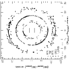
Figure 1: Location of pure parallel fields relative to targets in primary observations. Instrument of HST primary as indicated by symbols.

We illustrate in Figure 1 the difference in pointing between the parallel and primary observations for all pure parallel fields in the MDS database, using different symbols for each primary instrument. The WFPC2 field is on average 4.5, 8.2, 12.1, 7.1, and 5.3 arc min away from the FOC, FOS, FGS, STIS, and NICMOS primary target respectively.

Figure 2: Hours of pure parallel WFPC2 observations over the 4 years of the Medium Deep Survey. Program as indicated by shading.

About 25 hours of pure parallel exposure was obtained each month, giving a steady flow of observations. The database was supplemented using the archival data from primary observations which satisfied the survey criteria.

The observation history is illustrated in Figure 2 as an indication of the quantity of HST data that was available for the survey. There was a significant drop in the number of WFPC2 parallels after SM97 as a result of the dithered observing strategy of NICMOS and STIS primary observations. The pure parallel GTO data was available to REG as a WFPC2 Investigation Definition Team member and Windhorst’s Blue Survey data (WBS) was available from the HST archive 3 months after observation.

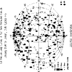
Figure 3: Distribution of the MDS pure parallel WFPC2 fields over the sky in Galactic Coordinates. Symbol size proportional to total length of exposure and are filled for fields processed for MDS.

The HST MDS (Griffiths et al. 1994a ), with over 400 random WFPC2 fields distributed over the full Sky, the GWS (Groth et al. (1994)) with 28 contiguous WFPC2 fields and the Hubble Deep Field (HDF Williams et al. (1996)) are datasets which give three very complementary samples of field galaxies at faint magnitude. The HDF gives depth in a single WFPC2 field, the GWS gives a larger area uniformly observed, and the MDS samples the whole sky as illustrated in Figure 3. All three sets have been analyzed uniformly through the MDS pipeline analysis software system.

Priority	Description
1	3 or more images in each of 2 or more Filters
2	2 or more images in each of 2 or more Filters
3	3 or more images in 1 Filter
4	2 images in one and 1 image in other Filter
5	1 image each in 2 Filters
6	2 images in 1 Filter
7	1 image only
8	Bad exposure
9	Failed observation

Table 1: Assignment of Field Priority in the MDS pipeline

MDS and GTO observations were primarily done with the F814W and F606W broadband filters. When more than 3 exposures could be taken with each of these filters, then F450W observations were taken in addition to those in the first two. In order to achieve a similar signal-to-noise ratio in the images taken in all three filters, the exposure times in F814W and F606W were requested to be about equal while in F450W the requested exposure was about twice as long. However, all WFPC2 observations in the MDS were taken in “non-interference” pure parallel mode (Griffiths et al. 1994b ), with the result that exposure times were of varied duration, with a variable number of exposures in the stack used for cosmic ray removal.

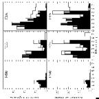
Figure 4: The total hours of exposure and number of fields at each priority (see Table 1) in each of the 3 primary WFPC2 Filters. The filled region of histogram are of fields processed through MDS pipeline. The partial shaded region is of non-survey fields.

Each field was given a priority based on the number of exposures available, as listed in Table 1. The total hours of exposure and the number of fields at each priority in each of the 3 selected WFPC2 Filters is illustrated in Figure 4. Practically all of the higher priority data has been processed through the MDS pipeline and made available in the MDS website. The single exposure, single filter fields were given lowest priority because of the inability to remove cosmic rays and the lack of any color information. After October 1995, the MDS used only pure parallel opportunities in which a minimum of two exposures with total exposure time longer than 20 min could be taken in each of two filters, or one exposure with a total exposure time longer than 30 min in each of two filters. Special data processing code was developed to perform cosmic ray rejection using exposures through different filters. This procedure, although better than attempting to clean cosmic rays from a single exposure, is performed at the cost of losing any objects of extreme color.

The pure parallel observations per se have therefore been the biggest challenge in the task of building a database using a clean statistical analysis. We will use the GWS for many of the illustrated distributions, in order to avoid complicating the discussion with effects due to changes in data quality.

3 The signal-to-noise index $\Xi\$.

To characterize the ability of our method to extract quantitative parameter estimates we define an information index based on the signal-to-noise in the image. Since we are dealing with mostly extended images, the definition of the index is different from the signal-to-noise ratio generally used for point sources.

We first define a contour around an object by selecting the subset of contiguous pixels which each contain a signal that is at least $1\sigma$ above the estimated local sky (see appendix for details). The signal-to-noise ratio of each of these pixels is computed individually. We define the signal-to-noise index $\Xi\$ as the decimal logarithm of the integral sum of these ratios, and we have found this dimensionless quantity to be a good measure of the information content of the image, and we have used it to define thresholds within the image analysis procedure. For any particular field, exposure time and WFPC2 filter, $\Xi\$ is linearly correlated with the magnitude of an extended image. Furthermore, it has the expected slope of 1 magnitude per 0.4dex, as shown in Figure 5 for GWS observations through F606W. Point-like stars follow a different sequence at brighter magnitudes.

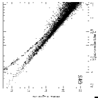
Figure 5: The decimal logarithm of the integrated signal-to-noise ratios of pixels within $1\sigma$ isophote ($\Xi\$) of extended images in GWS is linearly correlated with slope of 1 magnitudes per 0.4dex. Point-like stars follow a different sequence at brighter magnitudes. Symbols represent different models as indicated in Fig 22.

In most of the discussion on image analysis we will refer to $\Xi\$ rather than magnitude since it is a measure of image quality which can be used without reference to exposure time, sky background and filter used.

The MDS detection limit is at $\Xi\ \approx 1.6$, but the sample does contain some images with a smaller index, viz. those objects detected in the image of a different filter of the same region of sky. The completeness limit is at $\Xi\ \approx 1.8$ which is a half magnitude brighter than the detection limit. The morphology (disk-like or bulge-like) of galaxies can be determined for $\Xi\ \mathrel{\raise 1.29167pt\hbox{$>$}\mkern-14.0mu\lower 2.58334pt\hbox{$\sim$}}2.0$ and D+B models can be done for $\Xi\ \mathrel{\raise 1.29167pt\hbox{$>$}\mkern-14.0mu\lower 2.58334pt\hbox{$\sim$}}2.4$, which is 2 magnitudes brighter than the detection limit. To avoid any contamination by image noise the detection limit is set at a conservative level since that was already much fainter than the image quality needed to estimate morphology.

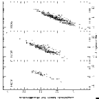
Figure 6: Limiting magnitudes for morphology classification ($\Xi\ \approx 1.8$) as a function of total exposure time for all fields processed in 3 primary WFPC2 Filters. The best fields with 3 or more images in stack are plotted as circles. The northern HDF field is the extreme point on each graph.

In Figure 6 we illustrate the limiting magnitude ($\Xi\ \approx 1.8$) as a function of total exposure time for all the MDS fields processed from WFPC2 pure parallel observations from HST Cycles 4 through 6, the GWS, the HDF, and archival cluster fields.

The GWS comprises 27 WFPC2 fields, each observed uniformly with 4 exposures in each of the I (F814W) and V (F606W) filters, with total integration times of 4400 and 2800 seconds respectively and one deep WFPC2 field with $\approx 25,000$ seconds in each filter. Our object catalog for the GWS has 12,800 objects in the 27 WFPC2 fields. The percentage of images with $\Xi\ \mathrel{\raise 1.29167pt\hbox{$>$}\mkern-14.0mu\lower 2.58334pt\hbox{$\sim$}}4.0,\ 3.0,\ 2.0\ \rm and\ 1.5$ is $0.3\%,4.6\%,30\%\rm and\ 67\%\$ respectively. In these survey images, $\Xi\ \approx 1.8$ corresponds to I=24.5 mag and to V=25.2 mag. From a catalog of $\approx 10,800$ galaxy images with $\Xi\ \mathrel{\raise 1.29167pt\hbox{$>$}\mkern-14.0mu\lower 2.58334pt\hbox{$\sim$}}1.8$ in both F814W and F606W, 11% of the images are fitted with two-component D+B models, 7% are classified as stars, 61% are classified as either disk-like or bulge-like, 20% are classified as generic galaxies (of uncertain disk or bulge nature) and less than 1% remain unclassified.

Figure 7: Average number of pixels in selected region and above $5\sigma$ and $1\sigma$ contours as a function of $\Xi\$ of images in GWS. We also show the number of pixels rejected as suspected residual hot pixels.

As illustrated in Figure 7, we find empirically that on average there are $10^{0.8\ \Xi\ }$ pixels above the $1\sigma$ contour, and $0.025\ 10^{1.1\ \Xi\ }$ pixels above $5\sigma$. When $\Xi\ \approx 2.0$ we thus have typically an image with 40 pixels above $1\sigma$ and 4 pixels above $5\sigma$. At the detection limit of our object-finding algorithm ($\Xi\ \approx 1.6$), we have typically an image with 15 pixels above $1\sigma$ and 1 pixel above $5\sigma$. Most images with $\Xi\ \mathrel{\raise 1.29167pt\hbox{$<$}\mkern-14.0mu\lower 2.58334pt\hbox{$\sim$}}1.6$ are of regions corresponding to objects which were detected in another filter and model fits on them are typically very poor.

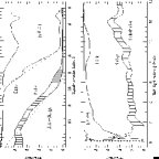
Figure 8: Fraction of images in GWS fields classified as different galaxy morphologies as a function of $\Xi\$ (upper panel) and as a function of half-light radius in pixels (lower panel) for images with $\Xi\ >2.0$.

In Figure 8a we show empirically that the fraction of images for which we can use the likelihood ratio (see sec 7) to determine whether the galaxy is more disk-like or bulge-like follows the relation $\min(\max(0,(0.82\ \Xi\ -1)),1)$. Of these galaxies, the fraction of images for which we can fit a significant two-component model follows the relation $\min(\max(0,(0.46\ \Xi\ -1)),1)$. Both these relations were derived by fitting a straight line to the slopes in this figure. We can classify about 60% of the galaxies with a $\Xi\ \approx 2.0$, and all of them with $\Xi\ \mathrel{\raise 1.29167pt\hbox{$>$}\mkern-14.0mu\lower 2.58334pt\hbox{$\sim$}}2.5$. Hardly any galaxy with $\Xi\ \mathrel{\raise 1.29167pt\hbox{$<$}\mkern-14.0mu\lower 2.58334pt\hbox{$\sim$}}2.2$ has sufficient signal to fit a two-component model, while 70% of them can be fitted at $\Xi\ \mathrel{\raise 1.29167pt\hbox{$>$}\mkern-14.0mu\lower 2.58334pt\hbox{$\sim$}}3.5$, of which however there are only very few examples in the MDS database. At $\Xi\ \approx 3.0$, about 40% of the galaxies are modeled as D+B . The saturation of the fraction at about 70% is probably the intrinsic percentage of galaxies which have a significant component in both disk and bulge.

In Figure 8b, we show a plot similar to Figure 8a, as a function of the half-light radius in pixels for images with $\Xi\ >2.0$. For over 90% of the images with a half-light radius $\xi\ \mathrel{\raise 1.29167pt\hbox{$>$}\mkern-14.0mu\lower 2.58334pt\hbox{$\sim$}}2$ pixels, the image can be classified statistically using the likelihood ratio (see sec 7) to determine whether the galaxy is more disk-like or bulge-like. We can fit a significant two-component D+B model to 20%, 25%, and 40% of the galaxy images with $\xi\ \mathrel{\raise 1.29167pt\hbox{$>$}\mkern-14.0mu\lower 2.58334pt\hbox{$\sim$}}$ 2, 5 and 10 pixels respectively. None of the galaxies with $\xi\ \mathrel{\raise 1.29167pt\hbox{$<$}\mkern-14.0mu\lower 2.58334pt\hbox{$\sim$}}2$ pixels had sufficient sampling to fit a two-component D+B model fit.

The ability and success of fitting models to an observed galaxy depend of course on both the integrated signal-to-noise index $\Xi\$, as well as the half-light radius of the galaxy in pixels $\xi\$. These two quantities are related to each other and to the morphology of the image. Systematic (or evolutionary) changes in the mean size and morphology as a function of apparent magnitude could slightly change Figure 8 if it were to be drawn for WFPC2 fields at significantly different limiting magnitudes. Figure 8 is applicable to exposures of about 1-hour in F814W and F606W. The difference in zero point magnitude for these filters is about the same as the mean color of galaxies, and therefore we can expect similar $\Xi\$ for the typical galaxy. We have excluded in this figure the galaxies imaged on the PC camera in order to keep the spatial resolution constant. Each WFC pixel is $0\farcs 1$.

4 Maximum likelihood estimation

Estimates of the centroid, magnitude, size, orientation and axis ratio of the observed galaxy image are initially evaluated using simple moments of the flux above the mean estimated sky, using those pixels within the $1\sigma$ contour. We next select an elliptical region around the object, ensuring that there are sufficient pixels to define the mean sky background to $\approx$ 0.5% accuracy (0.005 mag). Any pixels within the elliptical region which are associated with some other object and which are $1\sigma$ above the mean sky are cut out from the region analyzed, together with any pixels which have been flagged as “bad” in the calibration procedure (Ratnatunga et al. (1994)).

The procedure for the estimation of parameters via “maximum likelihood” starts by initial estimates of the model parameters from the observed moments of the image. For a given set of model parameters, the software creates a model image of the object and compares this image with the observations within the selected region (including the error image). The “likelihood function” is defined as the product of the probabilities for each model pixel value with respect to the observed pixel value and its error distribution; this function is evaluated as the integral sum of the logarithm of these probabilities. The likelihood function is then maximized by using a modified IMSL minimization routine (see Ratnatunga & Casertano (1991)). The 2D-image analysis used an improved version of the software developed for pre refurbishment WF/PC data (Ratnatunga, Griffiths & Casertano (1994)), the catalog of which was presented in Casertano et al. (1995).

5 Model fitting

There are many types of empirical models that have been suggested over the years to represent galaxy profiles. We have decided in particular to use scale-free axisymmetric models with an exponential power-law profile which have been shown to fit the broad continuum of normal galaxies (de Vaucouleurs (1959); Freeman (1970)). This choice has many numerical advantages which are desirable in leading towards the development of a practical maximum likelihood fitting algorithm. Elliptical galaxies are assumed to have a $e^{-r^{1/4}}$ (bulge-like) profile, and disk galaxies a $e^{-r}$ (disk-like) profile. Each profile is characterized by a major axis half-light radius and axis ratio. Some well exposed images need to be modeled as the sum of two elliptical components.

For about 4% of the galaxy images with no central concentration, the images are better fit by a $e^{-r^{2}}$ (Gaussian) or even $e^{-r^{4}}$ profile in which the light distribution is both less centrally peaked and has no extended tail. The isophotes of some ellipticals may be Boxy-distorted (Bender et al. (1989)) rather than the elliptical models which have been currently adopted. We will explore these and alternative models for fitting the continuum of irregular galaxies in a future paper.

For a point-like stellar image (star or QSO), we need four parameters: sky background, centroid (x,y), and magnitude. For the extended images of galaxies, we need at least one extra parameter which measures the size of the image. Taking into account the image jitter (see discussion above) and any errors in the PSF, we have found it useful to adopt a Gaussian profile and to estimate a size parameter even for the point-like images, to be used as a star-galaxy separation index. This procedure also takes the stellar image analysis through the same convolutions as those done for galaxy images, enabling the likelihood functions to be compared, with some caveats. Errors in the adopted PSF would appear as an extended residual image following the model fit. This could make a bright stellar image significantly better fitted with a model image which includes an extended component. This is a particularly important issue when attempting to detect underlying galaxies in QSO images (see Bahcall, Kirhakos & Schneider (1995)).

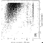
Figure 9: Plot of half-light radius in seconds of arc as a function $\Xi\$ for images in GWS. Symbols as in Fig 22.

In Figure 9, we show for the GWS dataset a plot of half-light radius in seconds of arc as a function $\Xi\ \mathrel{\raise 1.29167pt\hbox{$>$}\mkern-14.0mu\lower 2.58334pt\hbox{$\sim$}}2.0$. For most stellar images the estimated $\approx 0\farcs 02$ or $\xi\ \approx 0.2$ WFPC2 pixel. At brighter magnitudes with $\Xi\ \mathrel{\raise 1.29167pt\hbox{$>$}\mkern-14.0mu\lower 2.58334pt\hbox{$\sim$}}3.5$ we notice some larger objects (but $\xi\ \mathrel{\raise 1.29167pt\hbox{$<$}\mkern-14.0mu\lower 2.58334pt\hbox{$\sim$}}$ 1 pixel) which are very well separated from the sizes of galaxies. The PSF approximation adopted in the analysis is insufficient at these bright magnitudes. They could also be cases of stellar binaries which are just resolved and which at fainter magnitudes could contaminate the sample of objects classified as galaxies.

6 The parameters

We describe here the full list of model parameters in the order in which they are introduced as we increase the number fitted to an image. These are the intrinsic galaxy model parameters which are introduced before any PSF convolution or allowance for other instrumental effects such as (the small amount of) photon scattering in the CCD before detection.

(1) Sky Background.

The sky background is a very important part of the model estimates. A bias in the sky estimate could translate to a bias in the estimated morphology. Unlike for example Byun & Freeman (1995); Schade et al. (1996) we have therefore chosen to derive a maximum likelihood estimate for the mean sky background simultaneous with the other image parameters. We use sufficient pixels to ensure that the mean background sky is determined to an accuracy of 0.5%. Typical fluctuations of order 1% are seen in a single WFC frame. Some of this variation may be caused by the extragalactic background light (EBL) from faint unresolved galaxies. Much larger fluctuations are occasionally caused by the faint halos of nearby images, or by charge transfer problems caused by bright stars. The estimated sky backgrounds are seen to follow these variations very well. Sky background is assumed to be flat over the small region selected for analysis of each object.

In the procedure we have adopted, disk-like or bulge-like model fits could possibly converge with slightly different sky backgrounds within the measurement errors. By allowing the sky to vary, we are not imposing some prior choice of sky background. The error in the sky background is then properly reflected in the error estimates for the galaxy parameters and the likelihood ratio used for morphological classification.

(2,3) Centroid

The $(x,y)$ centroid of the model image is in most cases very close to the centroid of the observed image. The mean errors for $\Xi\ \approx$ 2.0 and 1.6 are 0.1 and 0.2 pixels respectively. The error becomes much larger for images fainter than the detection limit (i.e. $\Xi\ \mathrel{\raise 1.29167pt\hbox{$<$}\mkern-14.0mu\lower 2.58334pt\hbox{$\sim$}}1.6$). For the D+B models we assume the same centroid for both components. The software does allow an independent offset for the center of the bulge from that for the disk (parameters (12,13)), but this has not yet been fully investigated. The extra degree of freedom resulted in poor convergence in many more galaxies than in the few which justified it.

(4) Total magnitude.

The adopted magnitude is the analytical total magnitude of the galaxy model. This estimate has the advantage of not needing an aperture correction as is required for a fixed aperture or isophotal magnitude. However, since the magnitude integration is over a smooth galaxy image, small errors could arise from the fact that the model may not average properly over bright regions of star formation, for example. For D+B models the magnitude is the total for both components, a quantity better defined than the magnitudes of the individual components. The magnitudes of the individual disk and bulge components can be derived using the flux ratio ( ${\rm B/T\ }$ see below).

Note that the total magnitude is integrated theoretically out to infinity. For disk galaxies practically all (99%) of the light falls within 4 half-light radii. However for bulge-like galaxies only 85% of the light is within 4 half-light radii, and the model needs to extend out to 19 half-light radii to contain 99% of it. The Total magnitude for an elliptical could therefore be $\approx 15$% brighter than when calculated by integration out to a typical isophotal detection radius, and correspondingly for the ${\rm B/T\ }$.

(5) Half-light radius.

This is the radius within which half the light of the unconvolved model would be contained if it were radially symmetric (an axis ratio of unity). For axisymmetric galaxies, this definition is independent of the observed axis ratio of the galaxy, a parameter which depends on the intrinsic axis ratio and its inclination to the line-of-sight.

For point-like sources we fit a Gaussian profile with an exponent of 2.0, and the half-light radius is then 0.69 times the scale length. For disk-like galaxies with a profile exponent of 1.0, it is 1.68 times the exponential scale length. For bulge-like galaxies with a profile exponent of 0.25, it is the effective radius or 7.67 times the scale length. For D+B models it is by definition still the major axis radius within which half the light of the combined profile is contained. Like the total magnitude, this is a quantity better defined than the half-light radii of the individual components.

As a direct consequence of allowing the sky background to be a free parameter, we need to impose a maximum half-light radius in order to avoid this parameter from becoming meaninglessly large when a galaxy with no central concentration is fitted with a disk-like or bulge-like model. This limit has been set conservatively to equal half the maximum radius of the region selected for analysis. For $\approx 4$% of the galaxy images, the half-light radius converges on this limit, and those models need to be rejected and flagged for fitting with a less centrally concentrated model.

From numerical considerations we impose a minimum half-light radius of a tenth of a pixel on both the major and minor axes of a galaxy. For D+B models this minimum is imposed independently for each component. This assumption does not put any significant constraints on the axis ratio distribution of galaxies with a half-light radius larger than one pixel.

The quantity fitted is the logarithm of the half-light radius in seconds of arc. The half-light radius of the individual disk and bulge components can be derived using the bulge/(disk+bulge) flux ratio ${\rm B/T\ }$ and bulge/disk half-light radius ratio (see ${\rm HLF}\$ below).

(6) Orientation.

The adopted position angle is that of the axis of symmetry of the galaxy model. Measured in radians in the range $[-\pi/2,+\pi/2]$, this is set equal to zero when the source is assumed to be azimuthally symmetric with an axis ratio of unity.

For pre-refurbishment data with a highly asymmetric PSF, the observed orientation of the image could be significantly different from the intrinsic orientation of the fitted model. During the minimization procedure, the angle is measured clockwise from positive Y to positive X of the relevant CCD. It is then translated into a position angle as measured clockwise from North towards East using ${\rm PA}_{\rm V_{3}}\$of the HST attitude (pointing) vectors and the WFPC2 CCD plate-scale distortion map.

For D+B models we generally assume that the orientations of the disk and bulge components are the same. Since the bulge axis ratio is expected to be close to unity, any difference in orientation could be expected to be insignificant except in the brightest galaxy images. The software does allow for a difference in the orientation of the bulge from that of the disk (parameter(11)), but this too has not yet been fully investigated.

(7) Axis ratio

This is the ratio of the minor axis half-light radius to that of the major axis. This parameter has no units and is constrained to be smaller than unity to ensure proper definition of the major axis. For D+B models it is defined independently for each component. If the axis ratio cannot be shown to be significantly different from unity then it is held at unity; for the one-component case, the position angle can then also be dropped as a free parameter. The size of individual pixels also imposes limits on the ability to usefully constrain an axis ratio. Note that we adopt a minimum minor axis half-light radius of 0.1 pixel; i.e. for a Galaxy with a half-light radius of 0$\farcs$5 this imposes a lower limit on the axis ratio of 0.02 since WFPC2 has a pixel size of 0$\farcs$1 . In a few rare cases, this limit was useful for the prevention of the minimization procedure from converging on an unrealistically low axis ratio. This observationally imposed limit could be taken into consideration in an analysis of the axis ratio distribution, but can practically be ignored for galaxies with half-light radii larger than 1 pixel.

(8) bulge/(disk+bulge) flux ratio

This is the fractional flux contribution of the bulge-like component to the (disk+bulge) light ( ${\rm B/T\ }$) in the galaxy image. It has no units and ranges from zero for pure disk-like galaxies to one for pure bulge-like galaxies. The ability to estimate this quantity depends on the integrated signal-to-noise index $(\Xi\ )$ in the image. A larger $\Xi\$ is needed to separate out a second component with smaller fractional contribution to the total light (see Figure 17). A second component is only fitted when there is a significant improvement to the likelihood ratio to compensate for the increased number of parameters. The definition has used (disk+bulge) rather than Total to allow for the possible extension of the model parameter set to a third component such as a central point source (see Sarajedini et al. (1996)).

(9) Bulge axis ratio

This is the ratio of the half-light radius of the minor axis to that of the major axis of the bulge-like component. In D+B models it is often a poorly defined quantity when the disk component dominates the galaxy image, and the ratio is then adopted to be unity. We could not determine any meaningful relation between the bulge axis ratio and the disk axis ratio. Such a relation might have been expected if most disks and bulges have a typical axis ratio and were related by the common inclination to the observed line of sight. The latter does not seem to be the case.

(10) The ratio of the half-light radii (${\rm HLF}\$) bulge/disk

This is the ratio of the half-light radius of the bulge-like component to that of the disk-like component. We observed that the logarithm of this ratio has a weak correlation with the ${\rm B/T\ }$ flux ratio (see Figure 12). This correlation has been reported also by Kent (1985). For disk-like galaxies this ratio is about 0.25 and for bulge-like galaxies the ratio is about 1.6, i.e. on average, disk dominated galaxies have a disk half-light radius which is larger than the bulge half-light radius. Such is the case for our own Galaxy where this ratio is estimated to be about 0.65. However, there is a factor of 2.5 rms (i.e. one magnitude cosmic scatter) about the mean relation. It will be interesting to understand this relation using galaxy structure formation theories like those published by Mao & Mo (1998).

(11) Orientation difference of bulge from disk

See discussion above on Orientation.

(12,13) Centroid difference of bulge from disk

See discussion above on centroid.

7 Optimizing the model fitted

In brief outline the procedure is as follows:

The initial guess is typically far removed in parameter space from the final maximum likelihood model fit. At this point it is not useful to make any judgment about the selection of the model or the parameters to be fitted. However, testing has shown us that for 70% of a typical catalog with $\Xi\ \mathrel{\raise 1.29167pt\hbox{$<$}\mkern-14.0mu\lower 2.58334pt\hbox{$\sim$}}2$, we are never able to fit a significant D+B model. These images are analyzed only as stars or pure disks or pure bulge-like galaxies and the better model is selected. In Figure 8 we show a histogram of the number of galaxies as a function of $\Xi\$. We have highlighted the fraction fitted as D+B and the fraction for which we can classify the object as being significantly disk-like or bulge-like.

We first start with a disk-like model, or if $\Xi\ >2$ we attempt a 10-parameter D+B model fit. The first fit is a special quick mode of the minimization routine (modified IMSL 9.2 ZXMIN subroutine that uses a Quasi-Newton method). This mode of minimization is fairly fast since it does not attempt to check full convergence. It reaches a point in the multi-dimensional parameter space which is close enough to the final answer to investigate the likelihood function and make some intelligent decisions. These investigations are made after each minimization, and depend on the number of parameters that were fitted.

The quick mode does not use a higher resolution center (see Appendix). If a default resolution image had been used for the models, we investigate whether a high-resolution center will change the likelihood function. In over 75% of the tests in a typical catalog reaching down to the detection limit, the absolute change in the likelihood function is less than three, which can be considered as insignificant justification for the introduction of a higher resolution center. Since we are merging parts of two independently convolved images, the high-resolution center option is only used when needed.

If the half-light radius is less than $10^{-2.8+0.5max(\Xi\ ,3.6)}$ arc seconds, the program branches to test if the object is point-like. As discussed above, we fit a symmetric 5-parameter Gaussian model to allow for image jitter and any errors in the PSF. For most images the cut is at $0\farcs 1$ or one WFC pixel with a small increase for the brightest images (see fig 9). This test is done for about 30% of the objects in the sample, although only about 8% of the sample are eventually classified as probable point-like stellar sources, either stars or quasars. The star-galaxy classification is based on both the likelihood ratio for the best-fit galaxy model as well as the evaluated half-light radius for the object, which is typically 0.2 pixels (equal to the resolution used for the sub-pixel definition of the PSF).

The next check is to see if a two-component D+B model, if being considered, is significantly better than a single-component model with less parameters. In 60% of the cases (for $\Xi\ \mathrel{\raise 1.29167pt\hbox{$>$}\mkern-14.0mu\lower 2.58334pt\hbox{$\sim$}}2.0$) the numerical difference is less than 6 and this is insufficient justification for the fitting of a D+B model. If the half-light radius is less than two pixels we again select a single-component fit. In Figure 8b we show the fraction of galaxies as a function of half-light radius for which we can fit D+B models and the fraction for which we can classify the object as being significantly disk-like or bulge-like. The peak of the distribution for which we can fit D+B models is at about 5 pixels, and for obvious reasons we are not able to do so for galaxies with a half-light radius of less than 2 pixels. Even if the minimization gave a significant fit for a few of the latter galaxies, these fits are unlikely to be realistic models of these extremely under-sampled galaxy images.

For single component galaxies we next check if the axis ratio is significantly different from unity. If not, then it is set equal to unity, and a five-parameter symmetric model is fitted to the data. For all galaxies we fit both a pure disk as well as a pure bulge model, selecting the better fit model. If the absolute value of the likelihood ratio is smaller than four, then the classification as disk or bulge is not significant and these objects are classified as generic “galaxy”. If the object had been classified at a longer wavelength as disk or bulge, then the model output is selected to be that of the nearest wavelength for which the image was definitively classified. Otherwise, the model output is based formally on the likelihood ratio, ignoring the significance of it. For images with a sub-pixel half-light radius for which the likelihood ratio does not give a preference between star and galaxy, such objects are classified merely as “object”. The star-galaxy separation at sub-pixel half-light radii needs more detailed investigation, particularly for the purpose of attempting to isolate an uncontaminated sample of stars needed for modeling our own Milky-Way Galaxy.

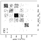
Figure 10: Comparison of the classification for images in GWS with $\Xi\ >2.0$ in the two observed WFPC2 filters F606W and F814W.

The image in each filter is modeled independently since the parameters in each filter need not be the same. In Figure 10 we compare the classification of images in GWS with $\Xi\ >2.0$ in both the filters F606W and F814W. Most of the objects received the same classification in the two filters. As expected from Figure 9 there is very little ambiguity in the star-galaxy classification.

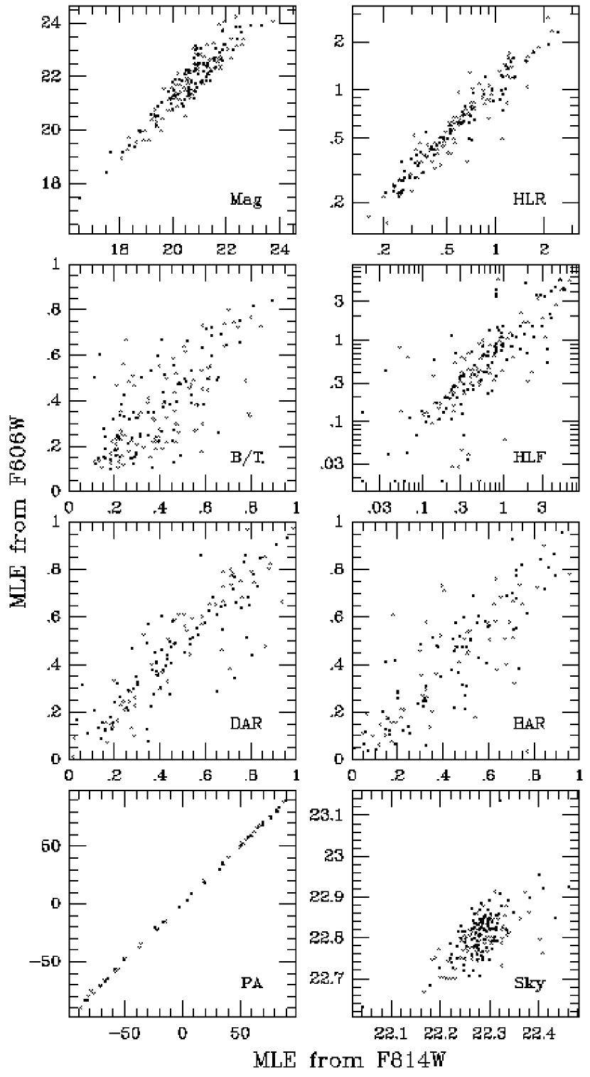
Figure 11: Comparison of the parameter estimates for about 150 galaxies in GWS which got full 10 parameter D+B MLE fits in both F606W and F814W filters.

In Figure 11 we compare the parameter estimates for about 150 galaxies in GWS for which there is a full 10 parameter D+B fit in both filters and a rms error estimate smaller than 0.5 in $log_{e}({\rm HLF}\ )$. The orientation (PA) is clearly the best defined parameter and this has proven very useful for studies of weak lensing (Griffiths et al. (1996)). The deviation for the total magnitude (Mag) is the color of the galaxy. The half-light radius (HLR) is the equal in the two filters for most galaxies. The axis ratios [for the disk components] (DAR) and for the bulge components (BAR) show scatter mostly from measurement error. The scatter in ${\rm B/T\ }$ flux ratio is real, and is caused by the different colors of the bulge and disk components.

For galaxies which demonstrably have two components, i.e. disk and bulge, the least well defined parameter is ${\rm HLF}\$ the ratio of the half-light radii. After a lot of effort, we have optimized an automated procedure to identify those cases for which a significant D+B model can be fitted. We are now able to select and converge (with over 90% success) on an unbiased estimate of the ratio of half-light radii for about half of these cases. The program determines if this quantity is unconstrained, by searching for a change in the likelihood as a function of this parameter. If the fainter component contributes less than 10% of the light, or if the axis ratio of both components is unity, then we have generally found this parameter to be poorly constrained. In Figure 12 we show that the logarithm of this parameter is a linear function of the ${\rm B/T\ }$ flux ratio with a correlation coefficient of about 0.5. Bulge dominated galaxies have a systematically larger Bulge/Disk half-light radius ratio (${\rm HLF}\$) than disk dominated galaxies. However the surface brightness limit for detection of the fainter component (see Fig. 20) probably contributes most of the observed correlation.

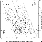
Figure 12: The observed correlation with 0.4 dex rms cosmic scatter, of the Bulge/Disk half-light radius ratio (${\rm HLF}\$) as a function of ${\rm B/T\ }$ flux ratio for galaxies in GWS. The mean value from relation (solid line) was adopted if ${\rm HLF}\$ is unconstrained. The dashed lines are at $\pm 0.7$ dex.

The scatter of 0.4 dex rms about the adopted mean relation (solid line) is equivalent to a cosmic scatter of one magnitude. If in the preliminary convergence the flux ratio ${\rm B/T\ }<0.1$, ${\rm B/T\ }>0.9$ or if the likelihood function was evaluated at extremes ${\rm HLF}\ \pm 0.7$ dex showed that the ratio of the half-light radius ratio was not constrained by the data, it is held fixed at the nominal value derived from the empirical relationship

$$\log_{10}({\rm HLF}\ )=-0.7+{\rm B/T\ }$$

Such relationships, although needed to facilitate convergence of the model fits at fainter magnitudes, are at best a rough approximation. However, when a parameter is unconstrained and the errors become comparable to the expected range of parameter space, this assumption does not significantly change the estimates of better defined parameters. The justification for the application of such a relationship is that it helps the routine to converge on a better defined minimum.

The program may also choose to fix the bulge axis ratio, or less frequently, the disk axis ratio at unity, if either of them is determined to be not different statistically from unity.

8 Estimated errors of parameters

The covariance matrix is the inverse of the Hessian i.e. the second-order derivatives evaluated at the peak of the likelihood function. When it is normalized to have unit diagonal elements, the cross-terms then give the correlation coefficients between the estimated model parameters. If the cross-correlation terms are not large, we can expect to derive reliable error estimates for the parameters from the diagonal elements. The parameters were selected to try to minimize the covariance between the fitted parameters described above.

In MLE theory, if the image being modeled is the same as the simple model assumed, then the parameter estimates and associated errors will be unbiased. However, real galaxy images which are well resolved are more complex than the simple axisymmetric image models that are assumed for MLE. The effects of spiral arms and bars on the parameter estimates are complicated and difficult to quantify using simulations. In general, we can expect that, given a sufficiently large sample, the cosmic dispersion caused by image peculiarities will be averaged out.

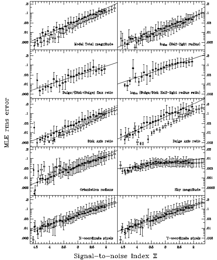
Figure 13: The running mean of estimated rms errors for parameters as a function of $\Xi\$ for single component and D+B MLE model fits for galaxies in GWS. See text for details.

In Figure 13 we illustrate a running mean of rms errors for parameters as a function of $\Xi\$. To first order, the logarithm of the rms error appears to increase linearly with $\Xi\$. The errors for single component and two component D+B fits are illustrated independently: in general, the latter errors are larger. There are a few points to notice. Firstly the sky error, of order 0.005 magnitude, is practically independent of $\Xi\$ and is defined by our choice of the number of sky pixels to include in the MLE. The orientation and centroid position, which were held the same for both components, show no significant increase in error than a single component fit at the same $\Xi\$. The errors in the bulge axis ratio are much larger for the two component fits. Since the rms of a random distribution between 0.13 and 1.00 is 0.25, rms errors larger than $\approx 0.1$ convey little useful information about the axis ratio. This occurs at a $\Xi\$ of 1.93 and 2.12 for single component disk-like and bulge-like galaxies and $\Xi\ \approx 2.25$ and 2.72 for the disk and bulge components in D+B model fits. The ${\rm B/T\ }$ errors do not become larger than 0.1 since a two-component model would not be significant if they did. The error in half-light radius is given in $log_{10}$ units. The error is 0.1 dex or 26% at $\Xi\$ values of 2.15 and 2.37 for single component and two-component models respectively. The ${\rm HLF}\$ ratio, given in $log_{10}$ units, is clearly the worst constrained parameter, requiring $\Xi\ \mathrel{\raise 1.29167pt\hbox{$>$}\mkern-14.0mu\lower 2.58334pt\hbox{$\sim$}}3.37$ for the expected error to be less than 0.1 dex or 26% rms.

The HDF superstack consisted of eleven individual HDF field pointings, and we can therefore use these to test the MLE method. We compare the MLE results for the HDF super-stack with the MLE results of the independent fits to the images of the same galaxies in each of the 11 sub-stacks. We limit the comparison to those galaxy images where the output from the sub-stacks resulted in the same morphology classification as that from the super-stack in the same filter. In the fits to all of the sub-stacks, we used the same object definition mask (see appendix) as that derived from object detection in the super-stack, together with the appropriate shifts.

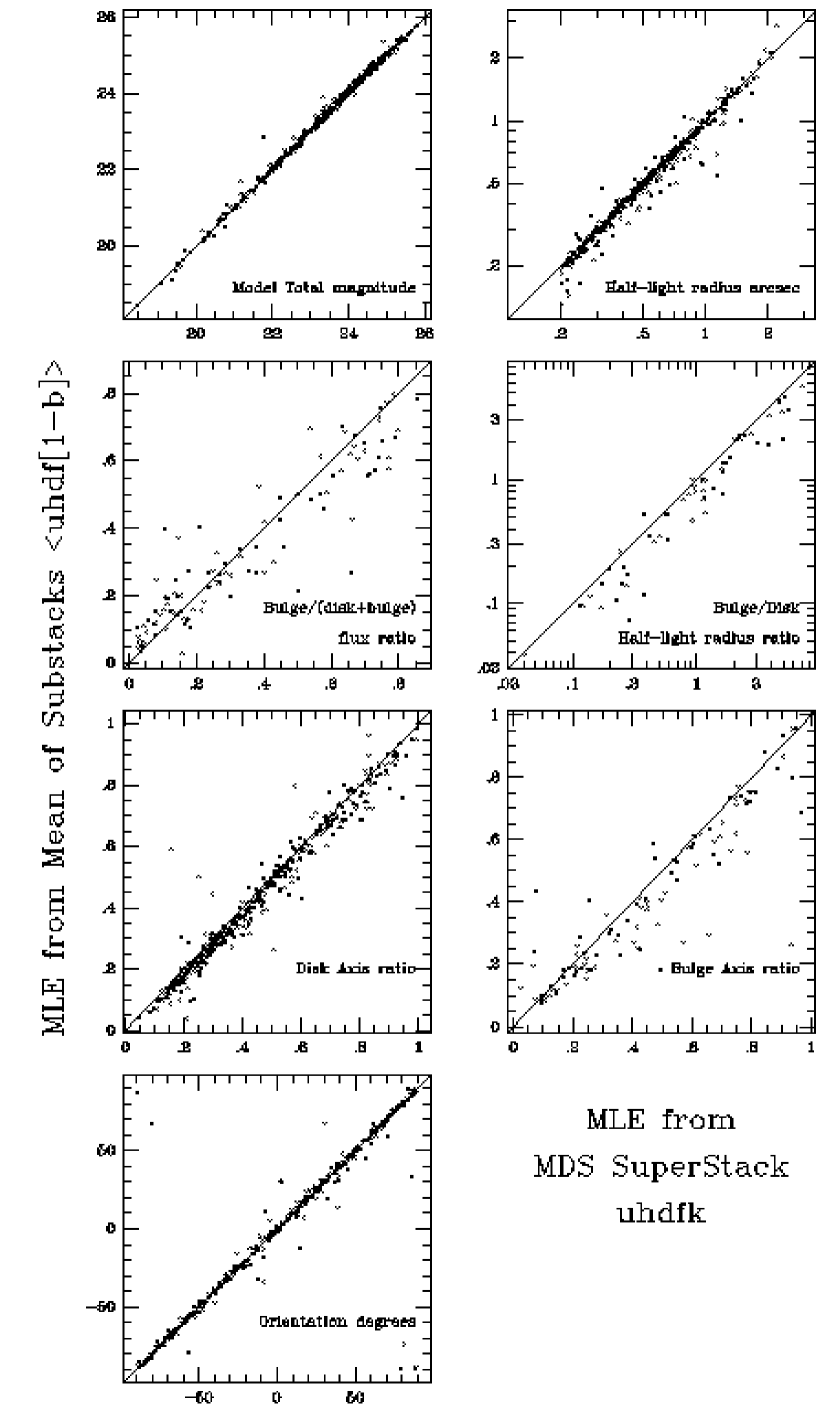
Figure 14: Comparison of parameter derived from our HDF super-stack (X-axis) with the weighted mean of the individual sub-stacks (Y-axis). See text for discussion of small systematic biases observed.

In Figure 14 we compare the MLE parameters derived from the super-stack with the weighted means from the individual sub-stacks. We notice a small systematic bias: the axis ratios in the super-stack are slightly rounder and the half-light radii slightly larger, with a slightly larger ${\rm HLF}\$ ratio. Our adopted approach to stack after shifting by closest integer number of pixels modifies the appearance of the peaked bulges. It will be instructive to see if the process of “drizzling” (Fruchter et al. (1997)) and stacking with sub-pixel shifts helps to remove this effect completely. The errors in flux values of pixels in drizzled images are not independent and to use our MLE approach, the covariance error matrix for each pixel needs to be included in the evaluation of the likelihood function. Software to do this has yet to be developed. For the brighter galaxy images in the HDF it is probably better to use a weighted mean estimate of the galaxy parameters from the individual HDF sub-stacks rather than the MLE values derived for the super-stack. Although the image bias in our HDF super-stack is disappointing, it does show the power of MLE estimates to be sensitive to the true nature of the images analyzed. Of course, all these problems can be avoided by not stacking the images at all and, instead, by summing the likelihood over the individual images (Ratnatunga, Griffiths & Casertano (1994)). This latter approach, however, is computationally impractical as yet.

Figure 13 allowed us to easily estimate an expected error for a given $\Xi\$. If the error estimate from inverting the Hessian is significantly smaller then it is unlikely to be real. This could happen for many reasons. There could be a sufficient covariance between parameters to make the diagonal only a small part of the error. The non-axisymmetric features of the galaxy image could have made a sharper dip in the likelihood function. The expected error could in fact be built into the evaluation of the Hessian at the peak of the likelihood function in order to pass over any sharp dips in the function. However, these relationships had not been derived at the time of the 1996-98 MDS pipeline processing. We find that a reasonable compromise for the current (October 1998) version of the database is to adopt a nominal expected error of half a magnitude brighter object if that is larger than the MLE error estimate from the Hessian. We find this is appropriate for all parameters except the orientation parameter, for which the original error estimates appear to be good. The orientation is not correlated with any of the other image parameters.

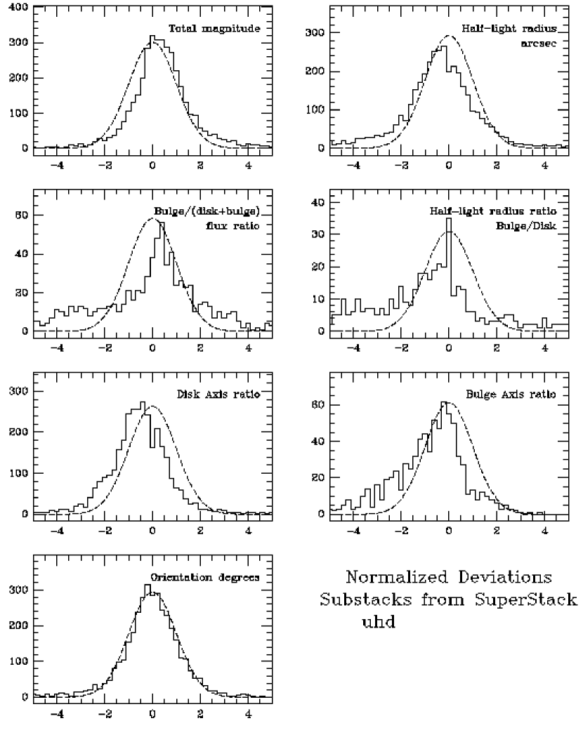
Figure 15: A histogram of the normalized deviations of the parameter estimates derived from the individual HDF sub-stacks from the value derived from the super-stack is compared with the expected standard normal distribution. See text for details.

In Figure 15 we show a histogram of the resulting normalized deviations of the parameter estimates evaluated in the individual sub-stacks from the value derived from the super-stack, and we compare the results with the expected standard normal distribution. The small bias caused by stacking the parameter estimates discussed above is clearly emphasized. We see a significant tail larger than normal for the ${\rm B/T\ }$ flux ratio and for the ${\rm HLF}\$ ratio because of the residual covariance in these parameters. The overall accuracy of the MLE parameter error estimates seems reasonable if we recognize that the simple galaxy model fitted does not include the structural detail seen in the real galaxy images at brighter magnitudes.

9 Selection effects effects due to Ockham’s razor

Since the adopted procedure fits the minimum number of parameters which are required to get a best MLE fit which is statistically significant, the parameter estimates reflect that decision.

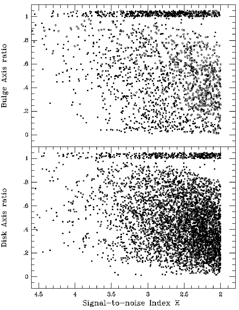
Figure 16: The Distributions of estimated disk and bulge axis ratios as a function of $\Xi\$ for galaxies in GWS. For illustration the face-on (axis ratio = unity) case has been distributed randomly in the finite range [1.00,1.05] outside the fitted range [0.01,1.00]. Symbols as in Fig 22. See the text for details.

In Figure 16 we show the distributions of disk and bulge axis ratios as a function of $\Xi\$. For illustration, the face-on case (axis ratio = unity) has been distributed randomly in the finite range [1.00,1.05] outside the fitted range [0.01,1.00]. The disk axis ratio appears to be randomly distributed within the range [0.10,1.00] for $\Xi\$ brighter than $\approx 3.0$. As images get fainter the axis ratios close to unity are found to be insignificantly different from unity. For example at $\Xi\ \approx 2$, axis ratios in the range [0.8,1.0] get set equal to unity, thus removing two parameters from the MLE fit. The same increase in errors produces a scattering of the observed axis ratios below 0.10. The bulge axis ratios show a similar distribution except that they are expectedly larger than the disk axis ratios. We also notice a number of small bulge axis ratios which are spurious and caused by barred galaxies which have not been properly included in the current MLE models.

Figure 17: The Distributions of ${\rm B/T\ }$ flux ratio as a function of $\Xi\$ for galaxies in GWS. For illustration, single component fits as pure disks ${\rm B/T\ }=0$ and pure bulges ${\rm B/T\ }=1$ have respectively been distributed randomly in the finite ranges [-0.05,0.00] and [1.00,1.05] outside the fitted range [0.00,1.00]. See text for details.

In Figure 17 we show the distributions of ${\rm B/T\ }$ flux ratio as a function of $\Xi\$. For illustration, single component fits as pure disks ${\rm B/T\ }=0$ and pure bulges ${\rm B/T\ }=1$ have respectively been distributed randomly in the finite ranges [-0.05,0.00] and [1.00,1.05] outside the fitted range [0.00,1.00]. The ${\rm B/T\ }$ flux ratio is distributed within the fitted range [0.00,1.00] for $\Xi\$ brighter than about 3.0, with the understood excess of disk like galaxies. As images get fainter, ratios close to zero and unity are not observed since these galaxies do not show a significant second component. The disk component in ellipticals is ‘lost’ before small bulges are lost in disk-like galaxies. For example at $\Xi\ \approx 2$, the observed ${\rm B/T\ }$ flux ratios are in the approximate range [0.1,0.6]

Figure 18: Distributions of ${\rm B/T\ }$ flux ratio as a function of half-light radius for galaxies in GWS. The distribution for single component fits are as in fig 17. See text for details.

In Figure 18 we show the distributions of ${\rm B/T\ }$ flux ratio as a function of half-light radius. The distribution for single component fits are as those in Figure 17. As galaxy images get smaller, the ${\rm B/T\ }$ flux ratios close to zero and unity are not observed since for these galaxies a significant second component cannot be resolved. Not unexpectedly, small bulge components in spirals can be inferred to have been lost from the MLE models of galaxies with half-light radii of a few pixels.

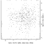
Figure 19: Distributions of Bulge/Disk half-light radius ratio (${\rm HLF}\$) as a function of $\Xi\$ for galaxies in GWS. See text for details.

In Figure 19 we show the distributions of the ${\rm HLF}\$ ratios as a function of $\Xi\$. For $\Xi\$ brighter than about 3.0 the ratio is seen to be distributed over a wide range. As images get fainter than those corresponding to $\Xi\ \approx 2.4$, the MLE routine does not estimate ratios larger than unity. This is because, as seen in Figure 17, the MLE program does not resolve disk-like components in faint galaxy images dominated by bulges.

We now look at the mean surface brightness within the central half-light radius ellipse. This has a constant magnitude offset from the central surface brightness of $-1.12463$ mag for disks and $-6.18126$ mag for bulges. The central surface brightness is a commonly quoted quantity, independent of axis ratio and inclination for our simple galaxy models. The advantage of discussing mean surface brightness here is that we find that the limiting mean surface brightness for morphological classification is a quantity which is about the same for disk-like and bulge-like components of the galaxy.

Figure 20: Mean surface brightness within the half-light radius ellipse as a function of major-axis half-light radius (left) and total magnitude (right) plotted independently for bulge (top) and disk (bottom) components. Cross symbol used for galaxies fitted with single component Model.

On the left-side of Figure 20 we show the mean surface brightness within the half-light radius ellipse as a function of the estimated major-axis half-light radius. In the case of D+B models, each of the components are considered separately. There is clearly a limiting magnitude for morphological classification which appears to be the same in each case, i.e. independent of whether it was a component of a D+B galaxy model, or a single component. We illustrate this for the GWS 4-stack images of 2800 seconds in F606W. A very similar graph is seen for F814W. There appears to be a slight numerical bias for MLE to converge on integer or half-integer half-light radii at the smaller values. This bias is presumably caused by our attempt to merge in a high-resolution center (see appendix).

On the right-side of Figure 20 we show the same surface brightness estimates within the half-light radius ellipse as a function of the total magnitude of the galaxy. Within the half-light radius ellipse of a galaxy or component, morphological classification can be done to a limit in surface brightness which is independent of the total magnitude of the galaxy up to certain magnitude limits. These two magnitude limits will be very useful as simple selection criteria in future models used to interpret the observed ${\rm B/T\ }$ distribution of galaxies and surface brightness dimming for cosmology.

10 Results

Preliminary versions of the MDS catalog have been the source of many scientific investigations: see, for example the papers on the size - redshift relation (Mutz et al. (1994)); angular size evolution (Im et al. 1995b ; Roche et al. (1996, 1997, 1998)) axis ratio distribution (Im et al. 1995a ); weak gravitational lensing (Griffiths et al. (1996)); luminosity functions of elliptical galaxies (Im et al. (1996)); morphological classification (Owens, Griffiths & Ratnatunga (1996); Naim, Ratnatunga & Griffiths 1997a ; Naim, Ratnatunga, & Griffiths 1997b ; Im et al. (1999)); galaxy interactions and mergers (Neuschaefer et al. (1997)); compact nuclei (Sarajedini et al. (1996)) the HST MDS cluster sample (Ostrander et al. (1998)) and a study of high-redshift clusters (Lubin et al. (1998)).

The catalog used in these analyses was mostly based on the star, disk or bulge model that best fit each object. Most of the previous analyses can be repeated on the new catalog and refined using the D+B models for the brighter sample. We do not, however, expect any significant changes to these previously reported results.

It is especially interesting to look at results on the two observables which have not been previously measured for large numbers of galaxies, especially in the magnitude range observed here, viz. the ${\rm B/T\ }$ flux ratio and the Bulge/Disk half-light radius ratio (${\rm HLF}\$). In fact we need to apply the same procedure to a large sample of bright nearby galaxies like those from the SLOAN digital sky survey (Gunn eta al. (1998)) in order to establish the behavior of these parameters on galaxies in the local universe.

11 Surface Brightness

Figure 21: The running mean of surface brightness as a function of total magnitude for galaxies in GWS (left) compared with HDF (right). Components from D+B models illustrated with thicker line follow same sequence as galaxies fitted with single component models. See text for discussion.

We have made plots similar to Figure 20 for much deeper observations such as the Hubble Deep Field (HDF). In Figure 21 we show a running mean of surface brightness as a function of total magnitude for the GWS galaxies on the left-side and compare it with those estimated for the HDF on the right-side. This graph illustrates Freeman’s result for disk galaxies (Freeman (1970)); the mean is the same, indicating that the observed distribution of surface brightness is intrinsic to the galaxies, with a cosmic dispersion of only about 1-magnitude. The expected trend of surface brightness dimming as the mean redshift increases for galaxies with fainter total magnitude is also seen. Correcting by $-1.12$ mag., we estimate that the mean central surface brightness of disk galaxies is 20.6, 21.4 mag in F814W, F606W for the GWS and 21.0, 21.8, 22.4 mag in F814W, F606W, F450W for the HDF. It is interesting that the mean surface brightness is the same for galaxies fitted as pure disk, as it is for the disk component of D+B galaxies. For bulges the scatter appears to be very much larger and our observations in GWS do not reach the limiting mean surface brightness bulges. Consequently, the mean for bulges in the HDF is about 2-magnitudes fainter than for bulges in the GWS fields.

12 Galaxy Color

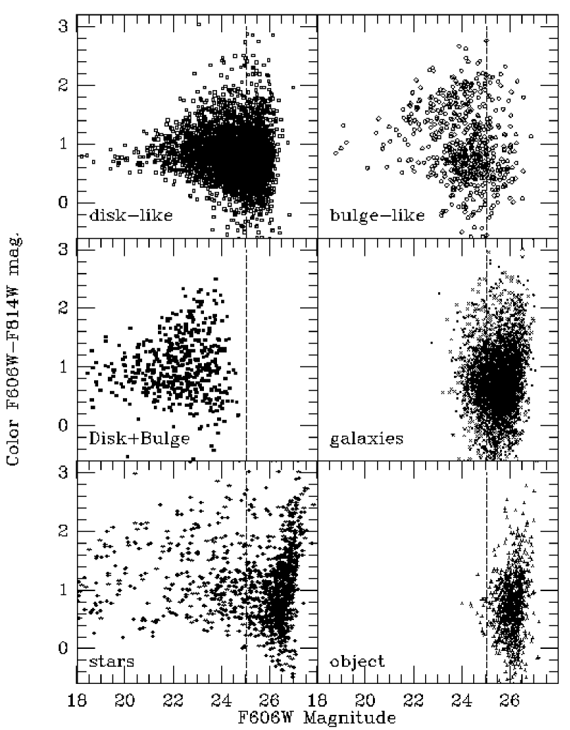
Figure 22: Color of GWS galaxies as a function of the F606W apparent magnitude. The dotted vertical line is drawn at the adopted the limiting magnitude for morphology classification at $\Xi\ \approx 1.8$.

In Figure 22 we look at the color of GWS galaxies as a function of the F606W apparent magnitude. We have shown all 6 classifications. The dotted vertical line is drawn at the observed completeness magnitude ( $\Xi\ \approx 1.8$ ). Most of the objects which were not classified morphologically are fainter than this limit. Furthermore, some of the images fainter than this limit and which have been classified as point-like are probably faint galaxies rather than stars. We have chosen not to filter the MDS catalogs brighter than this limit in order to avoid additional censorship of the sample in statistical analyses. All parameter estimates for galaxies fainter than this limit (i.e. magnitudes corresponding to $\Xi\ \mathrel{\raise 1.29167pt\hbox{$<$}\mkern-14.0mu\lower 2.58334pt\hbox{$\sim$}}2.2$) can be used for statistical analyses only, i.e. studies should not be focused on individual galaxies, particularly any outliers of such a distribution.

Figure 23: Color of the bulge-components of galaxies with the corresponding disk-components for galaxies in GWS which were fitted with D+B models in both F814W and F606W.

In Figure 23 we compare the color of the bulge-components of galaxies with the corresponding disk-components for GWS galaxies which were fitted with D+B models in both F814W and F606W. It appears that the colors of disk and bulge components of many galaxies are similar (the dotted line), although bulges are observed to be systematically redder, as expected, except for a few isolated cases.

Figure 24: The colors of the disk and bulge components as a function of the ${\rm B/T\ }$ flux ratio for galaxies in GWS

In Figure 24 we look at the color of disk and bulge components of galaxies as a function of the ${\rm B/T\ }$ flux ratio. As may be expected, the disk components of galaxies appear to become $\approx 0.5$ mag redder as we follow the plot from disk-like to bulge-like galaxies, with a cosmic scatter of 0.45 mag. The colors of bulges remain practically the same $\approx 0.2$ mag., with a larger cosmic scatter of 0.6 magnitudes.

Figure 25: The colors of galaxies in GWS as a function of the Bulge/Disk half-light radius ratio (${\rm HLF}\$).

In Figure 25 we look at the color of galaxies as a function of the ${\rm HLF}\$ ratio. It appears that redder galaxies have a smaller ratio. Careful statistical analysis is needed to ensure that this is “real” and is not caused by a selection effect in which the GWS galaxies were sufficiently bright that D+B models could be fitted to images in both F814W and F606W filters.

13 Conclusions

An automated maximum Likelihood procedure has been developed to calibrate, detect and quantitatively measure objects in the HST WFPC2 fields. The procedure measures the parameters of faint galaxies, despite the potential difficulties related to the undersampling in WFPC2.

D+B models are now fitted routinely to the brighter galaxy images as a part of the MDS pipeline. A D+B galaxy model, a pure disk, a pure bulge or a star model is chosen automatically using likelihood ratio tests. Classification is done for images with significant confidence.

Most HST MDS fields observed in 1994-1997 have been processed, resulting in a catalog of over 200,000 objects which have been put on the MDS website with a searchable browser interface. Clicking on a stack image will pick out and display the maximum likelihood model fit and the parameters for that object.

The statistical properties of the HST-MDS Catalog has resulted in many publications and comparisons with models of galaxy evolution will continue.

Appendix - MDS Pipeline

14 Association of WFPC data and MDS Field names

The MDS database was maintained and updated using Starview (Fruchter (1994)). Observations are assigned an alphanumeric 5-character name that is based on Galactic coordinates as described below such that fields which are from the same region of the sky are associated by name. The choise of the individual characters in the name is as follows:

1) The first letter of the name, ’u’, is the HST instrument letter assigned to WFPC2 observations. It was ’w’ for older WF/PC data.

2) Galactic Latitude from ‘a’ in the south to ‘z’ in the north in equal steps of sin(latitude), using numeric index [6-9,0-5] within 16$\buildrel{\circ}\over{.}$1 from the Galactic plane.

3) Galactic Longitude using sequence ‘1-5,a-z,6-9,0’ in steps of 10$\buildrel{\circ}\over{.}$0 such that numeric indexed fields are towards the Galactic Center. The Galactic caps within 3$\buildrel{\circ}\over{.}$9 from pole are assigned “a-” and “z_” SGP for NGP respectively.

4) Chronological sequence of primary target within the 31 degree² cells defined above, based on coordinates. Observations within a 0$\buildrel{\circ}\over{.}$5 radius are assumed to be of the same target.

5) Chronological sequence of Association around the same primary target set. These fields may overlap each other.

The program using a list of all pure parallel WFPC2 GO and GTO observations assigns the names. We have not included the STScI UV-survey program (pid=6253) or the current archive program (pid=7909) for all parallel WFPC2 data since February 1998. Every dataset in an associated group is allowed to be a maximum of 8$\farcs$0 (10% of WFC CCD width) from any other dataset in the same association. This range is sufficient to associate all WFPC data taken in parallel with a STIS or NICMOS observations, which are dithered, say within a 5$\farcs$6 square. For most cases the ${\rm PA}_{\rm V_{3}}\$orientation is identical. If it is not, then we ensure that the difference in rotation is less than 0$\buildrel{\circ}\over{.}$03 . This ensures a 1-1 mapping of the pixels, keeping any effect caused by the small rotation or differential distortion to be under about 0.5 pixels, the maximum error made by adopting integer truncated pixel shifts between images in a stack.

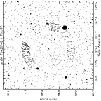
Figure 26: Repeat observations give a ring of pure parallel WFPC2 fields around FOS calibration star BD+28-4211.

Around some objects such as the FOS calibration star BD+28-4211 MDS has many repeat observations as illustrated on Figure 26.

15 Calibration procedure

Briefly, the calibration procedure is as follows.

The WFPC2 images are calibrated using the best available calibration data. We adopt the STScI static mask, super-bias and super-dark and flat field calibration files created for the HDF. Tables of hot pixels from STScI are used to correct fluxes in fluctuating warm pixels for the period of observation. Correction is made to ensure that the noise from any residual warm current is smaller than the read noise. Hot pixels, which cannot be corrected to that accuracy, are rejected. Saturated pixels and pixels with large dark current are flagged as bad and ignored. No attempt is made to interpolate over them. The software has been specifically developed to recognize the existence of missing pixel values.

In general we have more than one exposures in the same filter, in the same field, to reject the numerous cosmic rays by stacking exposures with a $3\sigma$ clip. We use a corrected version of the IRAF/STSDAS combine task. See Ratnatunga et al. (1994) for a detailed discussion of various aspects of the stacking procedure and the statistical errors which are corrected in the “combine” algorithm. A error image is also generated which computes the rms error from the noise model, taking proper account of pixels rejected by cosmic rays, the dark current, flat-field.

Shifts between images were determined by cross-correlation of the images. The coordinates listed in HST WFPC2 image and/or jitter file headers are often found to be insufficiently precise for the process of image stacking (Ratnatunga, Ostrander & Griffiths (1997)). The shifts are determined to an estimated rms accuracy of 0.1 WFC pixels. To avoid interpolation (which spreads the charge from cosmic rays, charge that is otherwise well confined), exposures are stacked with shifts corresponding to the nearest integer number of pixels, without any rotation or drizzling. Drizzled images (Fruchter et al. (1997)) are most useful for very deep exposures like the HDF, which do not occur in pure parallel observations. Drizzling causes the errors in adjacent pixels in the image to become correlated and significantly complicates a proper statistical analysis of the image.

A mode offset is employed to allow for changes in the sky background in different exposures due to changes in the fluorescent glow and scattered Sun/Earth light. The calibration accuracy is partly limited by the fluorescent glow. This can contribute as much as 50% of the dark current, and is strongly correlated with the cosmic ray activity during the WFPC2 exposure, which in turn depends on the particular orbit. However, except for very deep stacks like the HDF, the noise created by improper correction of this fluorescent glow results in a term which is small compared to other noise terms.

We next remove any large-scale gradient from the faint outer regions of bright galaxies, for which the nucleus was probably the target of the primary observation. The four CCD images of the WFPC2 are first oriented and merged along the pyramid edge and a single 2nd order 6-parameter polynomial surface is fitted across all four. This surface is then subtracted from each of the individual images and this automated procedure is iterated 2 or 3 times until no gradient is visible. Only about 4% of the processed MDS observations required this gradient removal.

After stacking, the image is multiplied by a selected factor, which is a power of 2, followed by an integer truncation and division by the same factor. This makes the images compressible without any loss of useful information, since the differential values before and after this process are much smaller than either the accuracy of the calibration or the averaged read-noise. The selected power depends on NCOMB, the number of images stacked and we adopt the function ${\rm nint}(\log_{2}(8\ {\rm NCOMB}))$, i.e. $2^{3}$ for a single image and $2^{6}$ for a deep 6-stack. The estimated rms error has an expected dynamic range of 0 to 25 ADU and the accuracy is unlikely to be better than 0.01 ADU. Therefore the rms ADU error image is multiplied by 100 and truncated to the nearest integer, in order to generate a short Integer image which is half the size when uncompressed than the size of the corresponding image of real numbers.

16 Object detection

The MDS pipeline was used to process only the typical field in which crowding was not a problem. We selected sparse fields in which the number of pixels $4\sigma$ or more above sky is typically under 5% of the total pixels in the field. We classified as non-survey and excluded from the MDS pipeline image analysis all low galactic latitude fields with lots of stars, and those fields close to Globular Clusters and local Group galaxies with, say, more than about 1600 objects detected. Non-Survey MDS fields were analyzed independently by other members of the team.

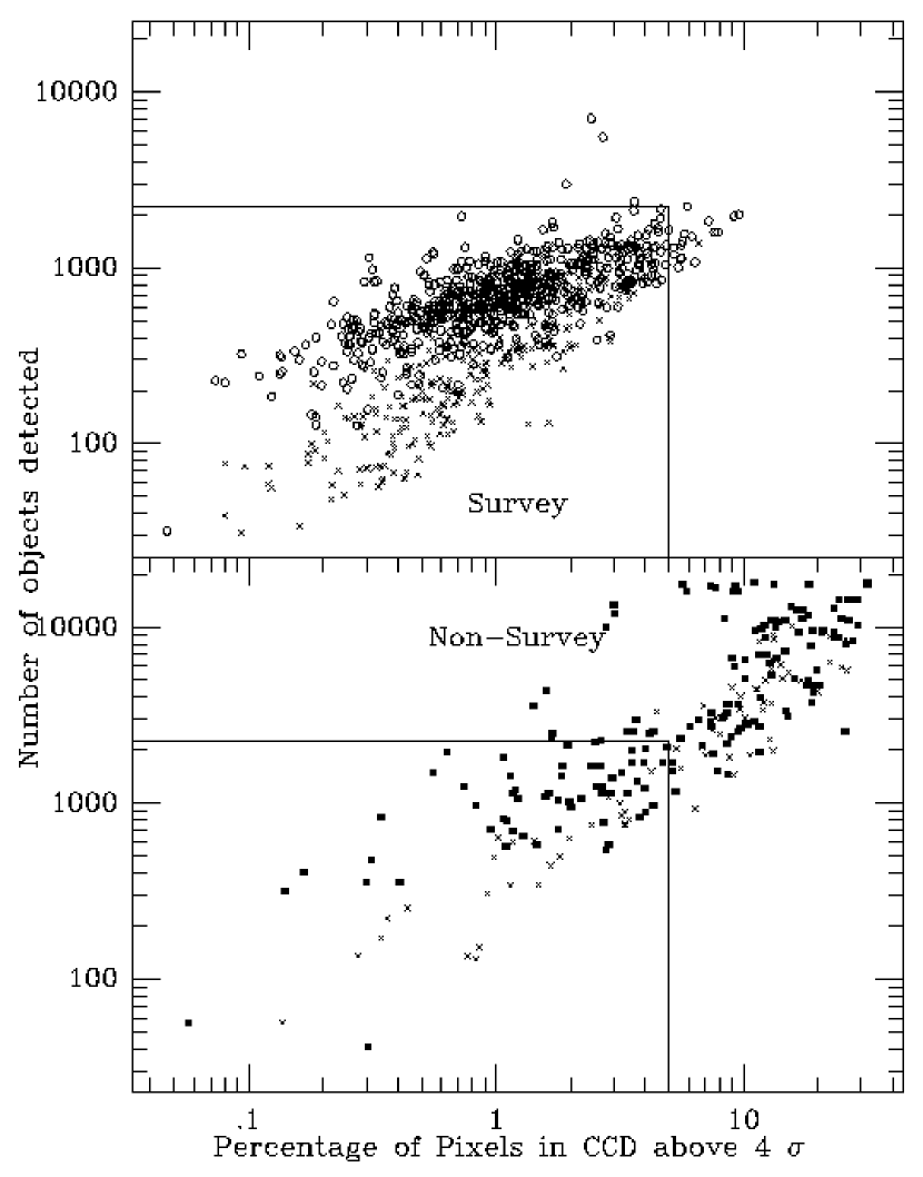
Figure 27: Number of objects detected as a function of of pixels above $4\sigma$. The fields selected to be part of MDS survey have less than about 5% of pixels above $4\sigma$. WFPC2 images with no cosmic-ray split have been indicated with crosses to show the systematic smaller number of object detections because of the attempted cosmic ray cleaning.

In Figure 27 we illustrate the number of objects detected as a function of the number of pixels above $4\sigma$. The figure shows that most of the fields selected as part of the MDS survey have a smaller fraction of pixels over $4\sigma$ and a smaller number of objects detected than in non-survey fields. In both cases, images with no cosmic-ray split have been indicated with crosses and show a systematic smaller number of object detections because of the attempted cosmic ray clean out.

Objects are located independently on each image using a ‘find’ algorithm developed for HST-WFPC data. This algorithm does not do any pre-convolution of the data, so that it is specifically designed to be insensitive to hot pixels and missing pixel values. It is based on finding local maxima and mapping nearby pixels to the central object, and then selecting those detections which are significantly above noise. The detection threshold algorithm originally developed for pre-refurbishment WF/PC data was optimized for WFPC2. This resulted in the location of a practically identical list of objects in the overlapping region of three WFPC2 MDS parallel fields USA0[1-3] observed in June 1994. To ensure that we do not break up bright galaxies into small regions of star formation, we adopted an object resolution of $0\farcs 5$, and small regions within this radius were allowed to merge with a brighter center. A larger radius of $1\farcs 0$ was used for WF/PC data. This algorithm has been observed to locate real objects with as much or better efficiency as the FOCAS algorithm (Tyson & Jarvis (1979)), which was developed mainly for ground-based data.

The MDS ‘find’ algorithm generates both a catalog and a ‘mask’ image, which associates each pixel with one object. This is a short integer file since the MDS pipeline assumes that there are less than 10K objects in a single WFPC2 field suitable for analysis. The stacking and initial object location procedure is a fully automated first step of the MDS pipeline. After the initial find, we have the only interactive part of the operation. We first look at the exposure, and confirm that it satisfies our requirements on inclusion into the MDS. A typical MDS survey field is uncrowded, with about 400-800 objects detected in the 5 arc-min² field. We also exclude from the MDS catalogs those objects with a centroid within 10 pixels ( $1\farcs 0$ ) from the pyramid and CCD edge, thus reducing the area surveyed by about 5% from 5.03 arc-min² to 4.77 arc-min² per WFPC2 field, and causing a $2\farcs 0$ wide gap in the shape of a cross in the center of each field. Rapid changes in the image distortion and the PSF ( a residual consequence of the original HST Spherical Aberration ) make the edge a very difficult region for reliable quantitative analysis.

The next operation is to fix up the mask for any bright objects which have been over resolved, or to delete any ghost images or extremities of bright stellar diffraction spikes which have been spuriously detected as objects. The detection algorithm has been optimized to work best at intermediate to faint magnitudes at the cost of over resolving a few bright objects. The numbers plotted in Figure 27 are raw counts before cleanup. The spurious detections are flagged with an interactive cursor for rejection or merger with the central image. This interactive operation takes about 30 min per stack and is done with a well defined set of guidelines which were originally developed for WF/PC data and modified appropriately for WFPC2.

The object detections in the various filters are then matched by software, and a single catalog is created, together with a revised mask for each image, so that corresponding pixels in the different filters are associated with the same object. Looking at a grid of the individual object detections, the final masks are inspected and the procedure is iterated as required to ensure that the object definitions as encoded by the final masks are acceptable. This is the conclusion of the calibration and object detection phase of the MDS pipeline.

The object detection algorithm and search thresholds were kept unchanged over the four years of the MDS. When new calibration data became available we recalibrated the data and created a new stack to obtain a slightly lower noise in the image. We however do not redetect objects, however. The masks remain constant, and after the field has been setup in the MDS database, model fits to any objects can be reprocessed with practically no human intervention. When there has been a significant improvement in the calibration or the fitting software, the whole database is reprocessed to obtain an improved version of the catalog, which is uniform over the whole period of observation. This has, however, become practical only after we obtained a SPARC Ultra-1, which on its own can do the reprocessing of the current database of over 400 fields in about two months. All of the MDS fields have been reprocessed with the last (July 1996) version of the MDS image analysis software. The shifted stacks were refitted after they were improved in July 1997 using inter-image shifts derived from cross-correlation analysis.

17 Definition of the object region for analysis

Most galaxies are analyzed by picking out a 64-pixel square region centered on the galaxy. The very few images (on average about 3 galaxies per WFPC2 field or 0.67% of the catalog) which are larger are analyzed as 128-pixel square images and in an extreme case as 256-pixel square region. The integral power of two in the region size in pixels was chosen for efficient convolution of models by fast Fourier transforms (FFT).

An initial guess of the local sky background is determined from an algorithm that determines the sky using an adaptation of the iterative, asymmetric clipping procedure as described by Ratnatunga & Newell (1984). In the very few cases for which it is detected that the local sky is poorly defined (large rms and skew in distribution) then the global sky is adopted as the initial guess. We next use the mask of detected objects generated by the MDS ‘find’ program in order to define a $1\sigma$ contour around the object. This is done by selecting the subset of pixels which are next to each other and are $1\sigma$ above the estimated local sky.

Despite careful ‘dark’ calibration and correction for suspected hot and warm pixels, pixels with fluctuating dark current are seen to leave a few “hot” pixels in the image. Since they could contribute significant flux compared with the flux of some of the faint images, any isolated pixels in the region outside the $1\sigma$ contour and over $5\sigma$ above immediate neighbors were located and were assumed to be hot pixels and rejected. This algorithm detected hot pixels in only 25% of the images and in these cases found on average only 5-pixels in a 64 pixel square region (See Figure 7). These values are for the GWS taken with the WFPC2 before it was cooled down from $-78^{o}C$ in April 1994, and for which warm-pixel corrections are not available. There are many less hot pixels in the newer data taken at $-88^{o}C$.

The initial guess of the local sky and the choice of pixels within the $1\sigma$ contour associated with the object are factors which influence only the region picked out for analysis. The pixels within the $1\sigma$ contour get no different treatment when the likelihood function is integrated.

18 The observational error distribution.

The presence of cosmic rays makes the observational error distribution of the raw observation non-Gaussian. We have found that the cosmic ray contamination can be represented by a Weibull distribution with index 0.25. In theory, the likelihood function can be defined by taking the model all the way back through the calibration procedure in order to make the comparison by summing over independent raw observations without any stacking. If this is done, one can take proper account of the effect of telescope “breathing” which results in slight changes to the observed PSF. One can also allow for contamination by faint cosmic rays and even any analog to digital conversion errors (a problem mainly for old WF/PC data) on the observational error distribution (Ratnatunga et al. (1994)).

However, after extensive software development and investigation using simulations, we found that this analysis of raw observations and the use of a complex error distribution gained only about 0.15 magnitudes in quality of morphology classification over the very much simpler analysis of calibrating and stacking the image to remove cosmic rays and the assumption of a Gaussian error distribution. With the latter approximation the log likelihood function is equal to

$$-0.5(1+\log(2\pi))\chi^{2}=-1.42\chi^{2}.$$

Maximizing the likelihood function is then identical to minimization of $\chi^{2}$. We have currently chosen to use the simpler analysis since the very slight improvement in results does not justify the very large increase in computation.

19 Generation of model images for comparison with observation.

The creation of the model image is the most technical and computer intensive part of the procedure. On average, of order 700 model images are used by the minimization routine to converge on the best-fit model of a single object. Since our minimization routine uses derivatives, an efficient high precision algorithm is required. For under-sampled images like those from WFPC2, sub-pixelation is very important, particularly close to the central peak of the galaxy image. We have developed a procedure which is automatically optimized by the algorithm by testing the evaluated likelihood function on the image being analyzed. We find that for many images the central pixels of the model image convolution needs to be done in sub-pixel space, and then block averaged for comparison with observation.

20 The creation of the image.

In order to ensure that the evaluated likelihood is a smooth function of all the model parameters, require computation of the model image at much higher resolution than that observed, particularly in under-sampled regions close to the center. The image models we have adopted are scale free and have an axis of symmetry. In order to minimize computation and make use of this symmetry, we therefore first evaluate the image by adopting an origin at the middle of central pixel of the array. The outer regions of the image are evaluated without sub-pixelation. If the models are scale free, then the outer regions can be multiplied by a constant factor to obtain sub-pixeled values for the inner pixels.

For example, we generate an 81 pixel square image by first computing pixels outside the inner 27 pixel square. Using the axis of symmetry, only half these pixels need to be computed. Then each pixel outside the inner 9 pixel square and within the 27 pixel square region is integrated with 3x3 subpixelation by integrating the 9 pixels at 3 times the radius and using a scale factor appropriate for the selected model. Following this step, each pixel outside the inner 3 pixel square and within the 9 pixel square can be integrated with an effective 9x9 subpixelation, and the region outside the central pixel and within the inner 3 pixel square can be integrated with an effective 27x27 subpixelation. Finally the central pixel with an 81x81 subpixelation is integrated from the rest of the whole image and the contribution for the very central subpixel. In this way the model image that is created has a very high degree of subpixelation for the inner pixels at practically no extra computation. In this example, the central 64-pixel square region used gets computed as a 280 pixel square image with increasing subpixelation towards the center. The image is effectively computed at 39200 points at the cost of 2917 evaluations, more than an order of magnitude increase in speed. This approach of sub-pixelation can be used on any scale free model, even if not elliptical.

21 The Point Spread Function

Selection of the Point Spread Function (PSF) is not easy. The choice is between, using observed PSF’s of well-exposed stars, or model PSF’s from programs such as tinytim (Krist (1992)). Observed stellar PSF’s are under-sampled, have random observational errors, and are not always available close to the image being analyzed. A compiled grid of stellar PSF’s from various observations has systematic errors comparable to the small systematic errors seen in model PSF’s. tinytim PSF images have the added advantage of being able to be generated as a sub-sampled image without observational jitter or the scattering in the WFPC2 CCD photon detection (see below for details).

Convolution of the WFPC2 model image is best done in sub-pixel space where it is less under-sampled. Tinytim (Krist (1992)) PSF’s are evaluated with 3 and 5 times sub-sampling for the PC and WFC CCD chips respectively. The 267 square PSF images are stored in the same data file format as the observations in a 3 by 3 PSF grid for each chip, and centered on the image at the pixel for which they were evaluated. A PSF grid image data file is made for each filter used in the observations. In the image analysis we choose from the grid the PSF for which the center is nearest to the location of the object. A 3 by 3 grid is sufficient for the corrected optics of WFPC2. A 11 by 11 grid with no sub-sampling was used for pre-refurbishment WF/PC data for which under-sampling of the extended PSF due to the spherical aberration was relatively less of a problem than the rapidly changing PSF as a function of the location on the chip.

We have so far ignored the changes to the PSF caused by the gradual shift of the mean focus between resets (maximum of 6 microns) and the telescope breathing which has a rms of ( 3 microns ). This in itself is a complicated issue when a stacked image is used in the analysis. The focus of every exposure in the stack cannot be assumed to be the same. Simulations have shown that for typical extended images with a half-light radius larger than say 2-pixels, model parameters derived using slight changes to the PSF are well within the parameter error estimates. For extended images, deviation of a galaxy from the simple model assumed could give larger errors to the parameter estimates.

22 Convolution

Convolution is done with IMSL 9.2 FFT routines. For most images a 64 pixel square array is used. We correct for any aliasing by generating a 16 pixel square image with a factor of 4 lower resolution and convolving it at the center of a 32 pixel square image where the region outside the central 16 pixel square is set equal to zero. The flux which gets convolved out to this border region is a sufficient estimate of the alias, and subtracted appropriately from the convolution of the original 64 pixel square array which is not surrounded by a zero border to prevent aliasing. This correction procedure takes only 1.25 times longer, rather than the 4 times increase needed to surround the 64 pixel square array with a zero buffer, and doing a 128 pixel square array convolution.

The subpixelation chosen is such that the region of the image selected for analysis will fit within a 64-pixel square array at the subpixel resolution. However, for WFPC2 images this was found to be insufficient for many highly peaked images that also covered most of the 64-pixel square array without any subpixelation. In these cases, we generate a second image for just the central pixels at the sub-pixelation used for PSF and then convolve this image as a 32-pixel square array, and correct it for aliasing effects using a similar procedure as for the main image.

The high-resolution image replaces the central 5-pixel square region of the model image. Since the center region after convolution is at 5-pixel subpixelation, the image can be shifted to the required center and block-averaged to the observed pixel scale using a simple algorithm that assumes a uniform flux distribution within each subpixel. Including such a higher-resolution center takes factor of 1.25 longer in CPU time, and used as required based on changes to the likelihood function.

23 Scattering at time of photon detection in WFPC2 CCD.

There is a non-negligible probability that a photon will be counted in a pixel adjacent to that in which it should have been detected. For a highly peaked source such as a stellar image, the location of the centroid within a pixel will govern the spill over to the adjacent pixels. The photon detection scattering of the model image therefore needs to be done at the observed image resolution and cannot be incorporated within a sub-sampled PSF.

After shifting the center and block averaging down to the size of the observed pixels, the image is convolved by a 3-pixel square kernel to allow for the photon detection scattering in WFPC2 data. The symmetric kernel adopted has [center,side,corner] values of [0.75,0.05,0.0125] and is as recommended in tinytim 4.1. We have compared this kernel with an azimuthally averaged kernel like that which was recommended in tinytim 4.0 with elements [0.5628,0.0937,0.0156]. We find that the revised, more centrally peaked kernel yields better model fits to a sample of stars. However, the combination of PSF and scattering is still not perfect and leaves residuals of about 5% to 10% which are significant in the brighter images.

24 Image Jitter

Since the tinytim PSF models are generated without including any contribution from telescope jitter, the intrinsic half-light radius estimated for a point source is non-zero. For a WFPC2 primary pointing in fine lock we expect about 10 mas (milli-arc-seconds) of telescope jitter. However, for parallel WFPC2 observations it could be larger because aberration corrections made for the primary instrument are slightly different from those required for the WFPC2. Since jitter data is still not available for all WFPC2 observations, they have as yet not been incorporated them into the MDS pipeline ( see Ratnatunga et al. (1995) for details).

Shifts between images were determined by cross-correlation of the images. Any small sub-integer shifts between the images that are ignored in the stacking procedure would also increase the effective jitter in the stacked image. Pointing Errors of 10 mas are possible at the times of target reacquisition between consecutive orbits of the HST and 20 mas if the target is reacquired after some other observation.

Any systematic radial errors between the actual PSF for the observation and the tinytim PSF model would also translate to a larger effective half-light radius. We typically estimate about 20 mas for unsaturated stellar images, growing to as large as 60 mas for the very bright saturated stars. The half-light radius computed by the program is not corrected as yet for jitter this correction which not have any significant effect, except on those images with a half-light radius smaller than a pixel.

25 The flow chart of the fitting and the output files

The input data for the program are four STSDAS/GEIS images for each filter, the calibrated image, corresponding error image, object definition mask image, the PSF grid image, and an ASCII data file with keyword information about the pointing and global noise characteristics of each calibrated stack. These files are identified in the header of the catalog that then identifies the object to be analyzed by the group and coordinate of the centroid, together with the mask number. In a special mode, it is possible if necessary to identify a small group of adjacent objects resolved with different mask numbers as a single object in the analysis.

The program fits all available images of the object in the different filters and outputs an ASCII data file with the fitted parameters, covariance matrix and other information about the likelihood ratio, and the sequence of intermediate results and tests. Catalogs for all objects in a field or a number of fields can be obtained using a keyword search of these data files. Also created is a FITS data image for each object. This file has the format of a grid with a single row of 7 images for each filter, starting from the longest wavelength at the top and progressively shorter wavelengths below it.

From left to right the images on a single row are

(1) Full image area read from the stack as observed.

(2) Selected region for analysis, with any adjacent objects masked out.

(3) Maximum likelihood model image, following PSF convolution.

(4) Maximum likelihood model image.

(5) Residual image.

(6) Error image.

(7) Object mask image.

To make the FITS files short integer and compressible, the sky subtracted stack images and the residuals are multiplied by 10 and transformed to short integer. The error image and mask are in the integer format used for these images (see sec 15).

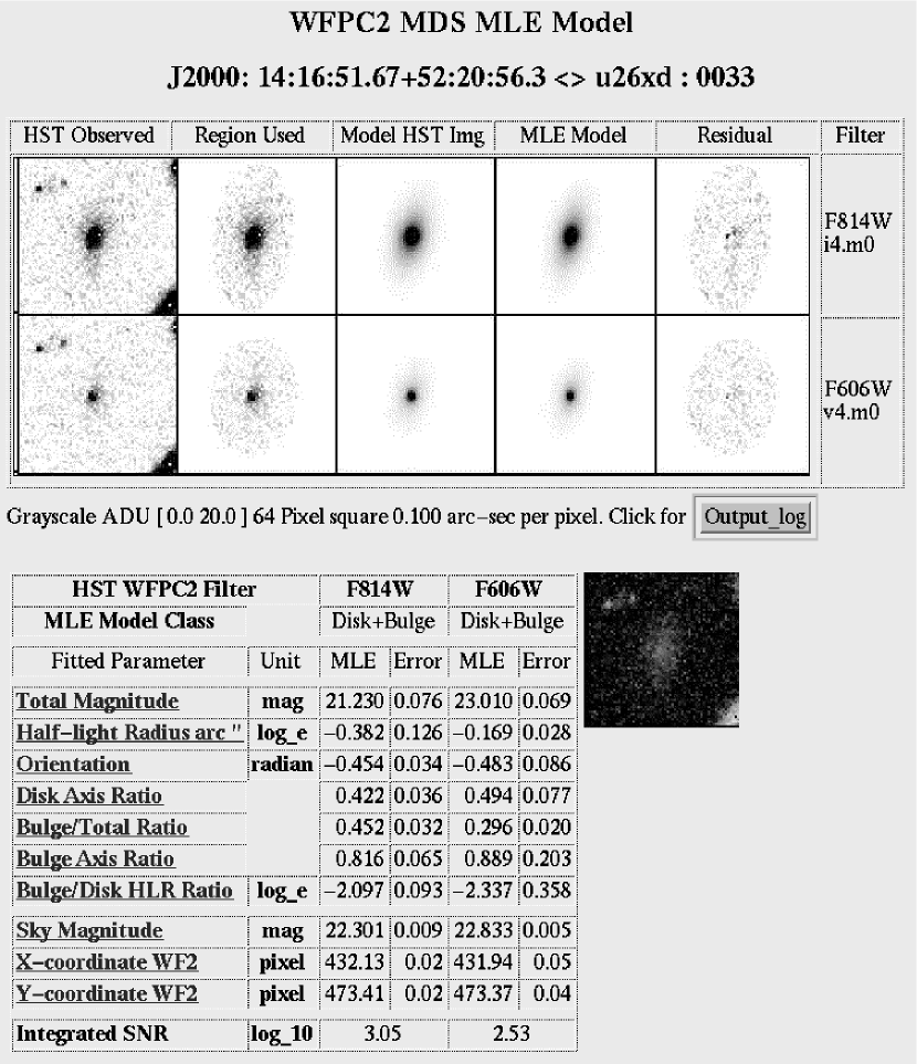
Figure 28: An example of a well exposed galaxy image from the MDS database as displayed via the MDS website. The dark image is in color and is generated from the available filters using fixed color transformation algorithm.

We show on Figure 28 an example of a well exposed galaxy image from the MDS database as displayed on the MDS website. Note that even the fainter F606W image which has $\Xi\ \approx 2.5$ is in the range signal-to-noise index which gives reasonable D+B decomposition.

As of October 1998 similar output for over 200,000 galaxies and stars had been made available on 19 CDROMS installed on a ‘Jukebox’ at STScI.

Analysis of an image as a star, disk-like or bulge-like galaxy is fairly straightforward. The only parameter that may be dropped is the axis ratio and in that case the orientation parameter is also not needed and the number of parameters fitted drops from 7 to 5.

The software can also use any profile index or even attempt to optimize its value as was done for images in the Uppsala galaxy catalog (Lauberts & Valentijn (1989)). However numerical simulations have shown that the profile index gives a measure of the ${\rm B/T\ }$ flux ratio only if the axis ratio of the two components are very similar. Else, the minimization procedure computes an index which is not within the range of one (for pure disk-like) and a quarter for (pure bulge-like). The value is often larger than two, as seen for the Uppsala galaxy catalog in which the index seems to have been constrained to be smaller than three for the same reason.

The D+B analysis is much more complicated. From the very choice and definition of the fitted parameters, to the automated selection of them to ensure convergence, has been a long investigation based on both fits to real data and to realistic simulations. Almost like the minimization process, getting close to the answer was much faster than checking and ensuring that the algorithm was optimum. Getting an algorithm that worked on a majority of the images has been tested and in use for sometime. The final optimization became practical with the aid of a SPARC Ultra-1 which is more than an order of magnitude faster than a SPARC-2 on which the programs were developed.

Automation gives uniformity at the cost of a few complicated cases (particularly at bright magnitudes) where a decision made by human eye would probably be different. The program was improved constantly till about July 1996 to reduce the percentage (currently about 2% ) of fits which are in error. All of the MDS database has been reprocessed with the improved version of the program logic.

References

- Bahcall, Kirhakos & Schneider (1995) Bahcall, J. N., Kirhakos, S. & Schneider, D. P. 1995, ApJ, 450, 486
- Bender et al. (1989) Bender, R., Surma, P., Doebereiner, S., Moellenhoff, C. & Madejsky, R. 1989, A&A, 217, 35
- Boroson (1981) Boroson, T. 1981, ApJS, 46, 177
- Byun & Freeman (1995) Byun, Y. I. & Freeman, K. C. 1995, ApJ, 448, 563
- Casertano et al. (1995) Casertano, S., Ratnatunga, K. U., Griffiths, R. E., Im, M., Neuschaefer, L. W., Ostrander, E. J. & Windhorst, R. A. 1995, ApJ, 453, 599
- de Vaucouleurs (1959) Vaucouleurs, G. de. 1959, Hdb. d. Phys., 53, 275
- Freeman (1970) Freeman, K. C. 1970, ApJ, 160, 811
- Fruchter et al. (1997) Fruchter, A. Hook, R. N., Busko, I. C. & Mutchler, M. 1997 in 1997 HST Calibration Workshop, ed. S. Casertano, R. Jedrzejewski. T, Keyes, & M. Stevens, p. 518
- Fruchter (1994) Fruchter, A. 1994, HST Archive Manual version 5.0
- (10) Griffiths, R. E., et al. 1994, ApJ, 435, L19
- (11) Griffiths, R. E., et al. 1994, ApJ, 437, 67
- Griffiths et al. (1996) Griffiths, R. E., Casertano, S., Im, M. & Ratnatunga, K. U. 1996, MNRAS, 282, 1159
- Groth et al. (1994) Groth, E. J., Kristian, J. A., Lynds, R., O’Neil, E. J., Jr., Balsano, R., Rhodes, J. & Idt, W. 1994, BAAS, 185, 5309
- Gunn eta al. (1998) Gunn, J. E., et al 1998, AJ, 116, 3040
- (15) Im, M., Ratnatunga, K. U., Griffths, R. E. & Casertano, S. 1995, ApJ, 445, L15
- (16) Im, M., Casertano, S., Griffiths, R. E., Ratnatunga, K. U. & Tyson, J. A. 1995, ApJ, 441, 494
- Im et al. (1996) Im, M., Griffiths, R. E., Ratnatunga, K. U. & Sarajedini, V. L. 1996, ApJ, 461, L79
- Im et al. (1999) Im, M., Griffiths, R. E., Naim, A., Ratnatunga, K. U. Roche, N. Green, R. F. & Sarajedini, V. L. 1999, ApJ, 510
- Kent (1984) Kent, S. M. 1984, ApJS, 56, 105
- Kent (1985) Kent, S. M. 1985, ApJS, 59, 115 astro
- Kormendy (1977) Kormendy, J. 1977, ApJ, 217, 406
- Krist (1992) Krist, J. 1992, The tinytim User’s Manual STScI
- Lauberts & Valentijn (1989) Lauberts, A. & Valentijn, E. A. 1989 in The surface photometry catalogue of the ESO-Uppsala galaxies
- Lubin et al. (1998) Lubin, L. M., Postman, M., Oke, J. B., Ratnatunga, K. U., Gunn, J. E., Hoessel, J. G., & Schneider, D. P. 1998, AJ, 116, 584
- Mao & Mo (1998) Mao, S. & Mo, H. J. 1998 MNRAS, preprint -ph/9805094
- Mutz et al. (1994) Mutz, S. B., et al. 1994, ApJ, 434, L55
- (27) Naim, A., Ratnatunga, K. U. & Griffiths, R. E. 1997, ApJ, 476, 510
- (28) Naim, A., Ratnatunga, K. U., & Griffiths, R. E. 1997, ApJS, 111, 357
- Neuschaefer et al. (1997) Neuschaefer, L. W., Im, M., Ratnatunga, K. U., Griffiths, R. E. & Casertano, S. 1997, ApJ, 480, 59
- Ostrander et al. (1998) Ostrander, E. J., Nichol, R. C., Ratnatunga, K. U. & Griffiths, R. E. 1998, AJ, 116, 2644
- Owens, Griffiths & Ratnatunga (1996) Owens, E. A., Griffiths, R. E. & Ratnatunga, K. U. 1996, MNRAS, 281, 153p
- Ratnatunga, Griffiths & Casertano (1994) Ratnatunga, K. U., Griffiths, R. E. & Casertano, S. 1994, in Restoration of HST Images and Spectra II, edited by R. J. and R. L. White, p. 333 Griffiths
- Ratnatunga, Ostrander & Griffiths (1997) Ratnatunga, K. U., Ostrander, E. J., & Griffiths, R. E. 1997 in 1997 HST Calibration Workshop, ed. S. Casertano, R. Jedrzejewski, T. Keyes, & M. Stevens, p. 361
- Ratnatunga & Casertano (1991) Ratnatunga, K. U. & Casertano, S. 1991, AJ, 101, 1075
- Ratnatunga & Newell (1984) Ratnatunga, K. U. & Newell, E. B. 1984, AJ, 89, 176
- Ratnatunga et al. (1993) Ratnatunga, K. U., Griffiths, R. E. Casertano, S., Neuschaefer, L. W., & Wyckoff, E. W. 1993, in Calibrating Hubble Space Telescope, ed. J. C. Blades & S. J. Osmer, p. 59
- Ratnatunga et al. (1994) Ratnatunga, K. U., Griffiths, R. E., Casertano, S., Neuschaefer, L. W. & Wyckoff, E. W. 1994, AJ, 108, 2362
- Ratnatunga et al. (1995) Ratnatunga, K. U., Griffiths, R. E. Neuschaefer, L. W., & Ostrander, E. J. 1995, in HST Calibration Workshop II, ed. A. Koratkar, A. & C. Leitherer, p. 351
- Roche et al. (1996) Roche, N., Ratnatunga, K., , R. E., , M. & Neuschaefer, L. 1996, MNRAS, 282, 1247
- Roche et al. (1997) Roche, N., Ratnatunga, K., Griffiths, R. E. & Im, M. 1997, MNRAS, 288, 200
- Roche et al. (1998) Roche, N., Ratnatunga, K., Griffiths, R. E., Im, M. & Naim, A. 1998, MNRAS, 293, 157
- Sarajedini et al. (1996) Sarajedini, V. L., Green, R. F., Griffiths, R. E. & Ratnatunga, K. 1996, ApJ, 471, L15
- Schade et al. (1996) Schade, D., Lilly, S. J., Le Fevre, O. Hammer, F., & Crampton, D. 1996 ApJ464, 79
- Stetson (1987) Stetson, P. B. 1987, PASP, 99, 191
- Tyson & Jarvis (1979) Tyson, J. A. & Jarvis, J. F. 1979, ApJ, 230, L153
- Williams et al. (1996) Williams, R. E., et al. 1996, AJ, 112, 1335
- Yee (1991) Yee, H. K. C. 1981, PASP, 103, 396