Measuring the Hubble Constant from Ryle Telescope and X-ray observations, with application to Abell 1413

Abstract

We describe our methods for measuring the Hubble constant from Ryle Telescope (RT) interferometric observations of the Sunyaev-Zel’dovich (SZ) effect from a galaxy cluster and observation of the cluster X-ray emission. We analyse the error budget in this method: as well as radio and X-ray random errors, we consider the effects of clumping and temperature differences in the cluster gas, of the kinetic SZ effect, of bremsstrahlung emission at radio wavelengths, of the gravitational lensing of background radio sources and of primary calibration error. Using RT, ASCA and ROSAT observations of the Abell 1413, we find that random errors dominate over systematic ones, and estimate $H_{0}=57^{+23}_{-16}$ $\rm kms^{-1}Mpc^{-1}$ for a an $\Omega_{M}=1.0,\Omega_{\Lambda}=0.0$ cosmology.

1 Introduction

Absolute distance measurements in astronomy are extremely valuable and are very difficult to make. The extragalactic distance scale in particular has profound implications for cosmology, but the distance-ladder methods have generated long-standing controversies. Direct methods of measuring cosmological distances, for example via gravitational lensing effects, offer alternatives to the distance ladder. One such method exists through combining X-ray observations of clusters of galaxies with the Sunyaev–Zel’dovich (SZ) effect [1972]. This method takes advantage of the fact that the SZ effect depends on a different combination of the intrinsic properties of the cluster gas (density, temperature, physical size) than the observed X-ray flux: hence the physical size of the cluster, and via the angular size, its distance, can be measured. To see how the distance depends on the measurable quantities, consider a blob of gas of size $l$, electron number density $n_{e}$, at temperature $T_{e}$. The observed X-ray flux density is

$$F_{X}\propto n_{e}^{2}f(T_{e})l^{3}D_{l}^{-2}$$

where $D_{l}$ is the luminosity distance and $f(T_{e})$ is the temperature dependence of the X-ray emissivity (including Gaunt factor). The SZ effect from the same gas is

$$\Delta T_{\rm SZ}\propto n_{e}T_{e}l.$$

If the blob subtends an angle $\theta$ then

$$\theta=l/D_{a},$$

where the angular size distance $D_{a}=D_{l}(1+z)^{-2}$. Rearranging,

$$H_{0}\propto D_{a}^{-1}\propto\frac{T_{e}^{2}F_{X}}{\Delta T^{2}f(T_{e})\theta},$$

where we have dropped the explicit $z$ dependence. $H_{0}$ can therefore be determined for a cluster of known redshift provided we can measure the gas temperature, the X-ray flux and the SZ effect, and provided we can model the distribution of gas in the cluster.

This method (e.g. Cavaliere et al [1979]) was suggested shortly after the SZ itself was proposed, and since the first successful detections of the SZ effect in the mid-1980s several authors have published determinations of $H_{0}$ based on it, using both single-dish (e.g. [1994, 1997]) and interferometric (e.g. [1995, 2000]) SZ measurements. Despite the advantages of the SZ method in by-passing the entire distance ladder, it does have its own sources of error, which must be carefully addressed. These include:

1. Beam switching that does not go fully outside the cluster; contamination by radio sources in the cluster or (for single-dish SZ measurements) in the reference beams; resolving out most of the total flux of the cluster (for interferometric measurements); poor spatial sampling of the cluster.

2. Errors in the temperature measurement of the cluster, due to poor photon statistics, temperature substructure and clumping of the cluster gas

3. Errors due to fitting a simplified smooth model of the gas distribution to a real complicated cluster

4. Biases due to selection effects in the chosen cluster sample.

In this paper we describe our analysis techniques for determining $H_{0}$ by combining SZ observations from the Ryle Telescope (RT) with X-ray data from ROSAT and ASCA. We apply this to data for the cluster A1413, for which we have previously published SZ results [1996]. Finally, we consider the various sources of error, both random and systematic, which affect our estimate.

2 Cluster modelling

We use our data to measure the Hubble constant by creating a numerical model of the temperature and density distributions in a cluster deduced from X-ray data, and then using these to generate mock RT data that can then be compared with real observations. The gas density is modelled as a King profile in one or three dimensions (depending on whether the cluster shows significant asphericity), and arbitrary temperature profiles can be specified. The cosmological parameters $H_{0}$, $\Omega_{M}$ and $\Omega_{\Lambda}$, upon which the relative scaling of the X-ray and SZ data depend, can be adjusted until both sets of mock data agree with the observations. The method is essentially similar to those used in other SZ measurements of $H_{0}$, especially other interferometric measurements [2000]. Unlike Reese et al we do not use the SZ data to constrain the shape parameters, as the X-ray image contains far more information and would dominate any joint fit; we do however allow for a non-spherical cluster.

2.1 Physical model

Our modelling is based on the analytical King approximation [1976] for the potential due to a self-gravitating isothermal sphere, which gives results consistent with X-ray images, at least in the inner parts of the gas distribution. The cluster total density $\rho$ at radius $r$ from the cluster centre is given by

$$\rho(r)=\rho_{0}\left(1+\left({r/r_{c}}\right)^{2}\right)^{-3/2},$$

where $r_{c}$is the core radius of the cluster. Assuming that the gas density, $\rho_{g}$ is related to the total mass density by $\rho_{g}\propto\rho^{\beta}$, then

$$\rho_{g}(r)=\rho_{g0}\left(1+\left({r/r_{c}}\right)^{2}\right)^{-3\beta/2}.$$ (1)

The average value of $\beta$ determined by fits to X-ray surface brightness of a large number of clusters is found to be $<\beta_{fit}>=0.67$ [1984], but we fit for $\beta$ separately for each cluster.

Although we typically use isothermal models for fitting X-ray and SZ data, we can vary the temperature to investigate specific effects. We do not vary the X-ray emissivity constant in these models; however, for typical rich cluster temperatures (7–10 keV) this constant is a weak function of temperature when observing in the ROSAT 0.5–2 keV band.

2.2 Simulating observations

We generate two-dimensional images, of typically $256\times 256$ pixels, of the model skies in SZ and in X-rays. This results in a spatial resolution in the model of $\sim 50$ kpc and a total simulation size of $\sim 10$ Mpc – numerical experiments show the results to be insensitive to these parameters. We can use either a spherical King model (equation 1) for the density, or a 3-d modification of it in which core radii ($r_{cx},r_{cy},r_{cz}$) are specified in three perpendicular directions, the directions relative to the plane of the sky being specified by three Euler angles. The density at a position ($x,y,z$) in these coordinates is thus given by

$$\rho=\rho_{0}(1+x^{2}/r_{cx}^{2}+y^{2}/r_{cy}^{2}+z^{2}/r_{cz}^{2})^{-3\beta/2}$$

We integrate the functions shown below along the rows of a three-dimensional array to generate the SZ brightness temperature and X-ray images:

$$\Delta T(i,j)=\sum_{k}n(i,j,k)T(i,j,k){{g(x)}\over{x^{2}}}{{k_{B}T_{0}\sigma_{T}}\over{m_{e}c^{2}}}L,$$ (2)

$$g(x)={{x^{4}e^{x}}\over{(e^{x}-1)^{2}}}\left(x\coth{x\over 2}-4\right),$$

$$x={{h\nu}\over{k_{B}T_{0}}},$$

$${\rm X}(i,j)=\sum_{k}Kn^{2}(i,j,k)t_{exp}L^{3},$$ (3)

where $T_{0}$ is the CMB temperature, $t_{exp}$ is the exposure time of the X-ray image and $K$ is a telescope, redshift and cluster-temperature dependent constant determining the received count rate, incorporating the bremsstrahlung and line emissivities, hydrogen absorption, detector bandpass and K-correction, expressed as ROSAT PSPC counts per second due to a volume of $1\rm m^{3}$ of gas, of electron density $1\rm m^{-3}$, at a luminosity distance of $1$ Mpc. $L$ is the size in metres corresponding to the angular extent of each pixel $\theta_{cell}$; this is calculated using the cluster redshift, $z$, and assumed values of $H_{0}$, $\Omega_{M}$ and $\Omega_{\Lambda}$.

We have checked that we obtain results consistent with the analytic expressions for both the X-ray and SZ profiles for the spherical isothermal King model. We choose not to use the analytic expressions in our code since the approach described above can more easily be modified to allow different distributions of gas density and temperature. For example, we have been able to investigate the effect of non-isothermal temperature profiles, and also central cooling flow regions. The latter have no effect on the SZ signal, however, since cooling flows are considered to be in pressure equilibrium with the rest of the cluster.

The brightness temperature decrement map is converted to flux density, multiplied by the RT primary beam response, and Fast Fourier Transformed to obtain the simulated aperture-plane response of the RT to the SZ decrement. The best-fit cluster parameters found for the cluster A1413 (see section 3.1) give a profile in the aperture plane for different observing baselines shown in Figure 1. Mock data that correspond to the real RT observations can then be generated by sampling this array at the observed coordinates in the aperture plane.

We also simulate the process of observing the sky with the ROSAT PSPC or HRI. The model X-ray sky is convolved with the X-ray telescope point-spread function, and a suitable background level added. For making model fits a smooth background is used; we can also make images in which each pixel value (signal plus background) is replaced with a sample from a Poisson distribution of the same mean, thus generating realistic X-ray images.

We tested the program to ensure that it gave the expected dependence upon central number density, $\beta$, core radius, gas temperature and value for $H_{0}$ and to check that the results for the simulations were not dependent upon pixel size or overall array size.

2.3 Predictions of SZ observations

We have predicted the effect that changes in various cluster parameters would have on our RT observations. In particular we were concerned about the behaviour of the flux density measured on the shortest RT baselines, since these are the most sensitive to the SZ effect. (The shortest physical RT baseline is $870~{}\lambda$, but at for lower declinations this can be projected down to a minimum of the antenna diameter of $640~{}\lambda$.) The results here were obtained using the model parameters for Abell 1413, but are typical of all the rich clusters we observe.

We simulated a cluster with using the best-fit parameters that we have found for A1413 (see section 3.1) but varied the core radius. We found that the central decrement is directly proportional to the core radius, as expected, and that the flux density measured on the 870 $\lambda$ baseline quickly began to flatten off (see Figure 2) as the RT starts to resolve out the SZ signal. This resolving out starts to become significant for core radii of greater than about 70 arcseconds for the 870 $\lambda$ baselines.

In a further test we varied the central number density, $n_{0}$, for various core radii to give the same observed flux density using a $870\lambda$ baseline, and recorded the central temperature decrement that these models would give. The results are also shown in Figure 2. The central decrement does not vary greatly with core radius, especially around 60 arcseconds which is the expected size for a cluster with core radius of about 200 kpc at moderate redshift.

We have also assessed the effects of redshift and cosmology on the SZ signal seen. We simulated observations of clusters with the same intrinsic parameters lying at different redshifts. First we calculated the clusters’ angular core radii, corresponding to a constant physical radius of 250 kpc, assuming Einstein-de Sitter ($\Omega=1.0$) and Milne ($\Omega=0.0$) cosmologies. The results for observations with baselines of 870 and 1740 $\lambda$ are shown in Figure 3. It can be seen that the RT has similar sensitivity to a cluster at redshifts between 0.2 and 10 on the shortest baseline in both cosmologies. On the 1740 $\lambda$ baseline the signal peaks for clusters at redshifts between 0.3 and 4 in an Einstein-de Sitter cosmology, but tends to a maximum value in a Milne universe beyond a redshift of 1. We therefore conclude that observations of the SZ effect with the RT should be possible for clusters at any redshift from $z=0.1$ to $z=10$.

Although the SZ effect predicted to be detected by the RT from a cluster of given physical size is largely independent of cosmology, the value of $H_{0}$ that we will calculate from observations will be affected by the values of $\Omega_{M}$ and $\Omega_{\Lambda}$ that we adopt. The true value of $H_{0}$ and the calculated value $H_{0}^{\rm calc}$ will be related by

$$H_{0}={{H_{0}^{\rm calc}D_{a}^{\rm calc}}\over{D_{a}}}$$

where $D_{a}^{\rm calc}$ and $D_{a}$ are the calculated and true angular distances to the cluster respectively. The correction factor $H_{0}^{\rm calc}/H_{0}$ is shown in Figure 4.

2.4 Fitting to X-ray images

Since ROSAT X-ray images contain far more information about the gas distribution in a cluster than RT SZ data, we use the X-ray image to model the density distribution. We assume the cluster is a triaxial ellipsoid with two principal axes in the plane of the sky, and with the core radius along the line of sight equal to the geometric mean of the other two core radii. We then use a downhill simplex fitting method, implemented by the routine amoeba [1986], to optimise the central density, core radii, ellipsoid centre, position angle and $\beta$ parameter. The likelihoods of the data given the model are calculated as the product of the Poisson likelihoods of obtaining the observed count at each pixel in the X-ray image, given the parameters. It is necessary to use the Poisson statistic rather than $\chi^{2}$ in order to avoid biases in the regions of low count rate where the two statistics differ significantly. This method also allows arbitrary regions to be excluded from the fit; this is used for example to exclude point sources in the X-ray image.

We use vignetting-corrected X-ray images (i.e. divided by the image of effective exposure time) for the fitting. Although this results in a distortion of the photon statistics across the map (partly due to the presence of the non-vignetted instrumental background), this effect is small in the central part of the image where all the cluster signal lies. We also use images that are binned so as to under-sample the PSF (pixel size equal to FWHM of PSF) so that the position dependence of the PSF is negligible over the region of interest.

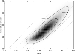
Figure 5: Greyscale and solid contours: likelihood of fit to X-ray data, as a function of $\beta$ and core radius of the major axis, marginalised over $n_{0}$ but with the axial ratio and position angle (which are very well determined) fixed. Contours are 67% and 95% confidence. Dotted contours: predicted mean flux density on the shortest RT baseline, for $h=0.5$. The degeneracy between $\beta$ and the core radius clearly has little effect on the predicted flux density, and hence on the fitted value of $H_{0}$.

There is a degeneracy between $\beta$ and $\theta_{c}$, and $n_{0}$, in that almost equally good fits can be obtained by changing the value of $\beta$, and re-fitting for $\theta_{c}$ and $n_{0}$. However, although the resulting value of the central temperature decrement is changed for these different fits, the flux density observed by the interferometer is almost unchanged. This is because the observed flux density depends on both the central decrement and the shape of the cluster, and on our most sensitive baselines the two effects almost cancel. The effect of this can be seen in Figure 5, which shows contours of likelihood of the X-ray fit in the $\beta$–$\theta_{c}$ plane overlaid with contours of the predicted flux density observed by the RT. The flux density contours (which are used to calculate $H_{0}$) lie parallel to the $\beta$–$\theta_{c}$ degeneracy, which thus has little effect on the value of $H_{0}$ found. Reese et al. [2000] find a similar result for the OVRO/BIMA arrays.

2.5 Fitting to SZ data

Interferometers measure the Fourier transform of the sky brightness distribution at discrete points defined by the orientation of the baselines, with independent noise values at each point. Inverting the data to form an image results in both signal and noise being convolved with the Fourier transform of the sampling function (the synthesised beam), resulting in long-range correlations across the map. With well-filled apertures and high signal-to-noise, this is not a problem. Since the RT has few baselines on which the SZ effect is detectable, these correlations are significant, ie the synthesised beam has large far-out sidelobes. It is therefore very difficult to do meaningful fitting to the data in the image plane. Accordingly, we fit our data to models in the aperture plane, although we also make maps, particularly in order to identify positive sources in the field.

Once a fit has been made to the X-ray image using an assumed value of $H_{0}$, an SZ sky model and simulated RT aperture are generated as described above. Variations in $H_{0}$ result in a simple scaling of the amplitude of the SZ signal. The calibrated, source-subtracted RT visibility data are read in and a $\chi^{2}$ statistic calculated between the real and mock data as a function of amplitude scaling; we multiply by a prior that is uniform in log space (since $H_{0}$ is a scale parameter) to find the peak and extent of the posterior probability distribution.

3 Calculating $H_{0}$ from A1413

A1413, at a redshift $z=0.143$, is a massive and highly luminous cluster with a ROSAT-band luminosity of $2.0\times 10^{38}$ W [1995]. We have previously published SZ data on the cluster Abell 1413 [1996] but did not derive an $H_{0}$ value there due to the significant ellipticity of the cluster and the presence of a moderate cooling flow, both of which complicate the process. Here we calculate $H_{0}$ from A1413 taking both these effects into consideration. As well as our RT SZ data, we use an observation made with the ROSAT PSPC, and a temperature derived from ROSAT HRI and ASCA data.

3.1 X-ray image fitting

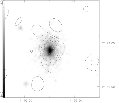
Figure 6: X-ray and SZ images of A1413, from Grainge et al (1996). The greyscale is the ROSAT PSPC image; it runs from 2 to 80 counts in a $15^{\prime\prime}\times 15^{\prime\prime}$ pixel. The contours show the Cleaned map of the naturally weighted RT 0–1 k$\lambda$ visibilities with restoring beam $169^{\prime\prime}\ \times\ 110^{\prime\prime}$ at position angle 2.7^∘; contour levels at $-450$, $-375$, $-300$, $-225$, $-150$, $-75$, 75 $\mu$Jy.

We fitted an ellipsoidal model (as described in section 2.4) to the ROSAT PSPC image observed on 1991 November 27, which has an effective exposure of 7696 s. We use only the hard (0.5–2 keV) data in order to minimise the effect of Galactic absorption; the image is shown in Figure 6, along with the RT SZ image. Allen et al. [1995] find that A1413 has a cooling flow with a mass deposition rate of 200 M${}_{\odot}\rm yr^{-1}$ within a radius of 200 kpc of the centre, and that the temperature in this region is depressed by some 20% from the value in the outer regions. Therefore we excluded the X-ray data within the cooling flow radius from our analysis, along with several X-ray point sources which appear in the image. Keeping the cooling flow region in the fit would result in a more compact model (higher $\beta$, smaller core radius) that would not reflect the true distribution of the gas, most of which is outside the cooling flow.

Allen and Fabian [1998] use ASCA and ROSAT HRI data to determine the temperature of A1413 in two models; one assuming the gas is isothermal, and one also fitting for a cool component, with the fraction of the total emission from the cool gas normalised by the fitted mass deposition rate of the cooling flow. These methods yield $7.5^{+0.3}_{-0.3}$ keV and $8.5^{+1.3}_{-0.8}$ keV respectively (90% confidence errors). The latter value is a better estimate of the temperature of the bulk of the cluster gas, outside the cooling flow region. Since we have excluded the cooling flow region from our fit to the surface brightness image, we use this higher temperature as the more consistent model. The value of $H_{0}$ that would be obtained from using the cooler temperature can be found from the scaling given in section 4.12. The X-ray emissivity constant was calculated assuming an absorbing H column of $1.62\times 10^{24}$ m^-2, a metallicity of 0.3 solar and a temperature of 8.5 keV, giving a value of $3.41\pm 0.24\times 10^{-69}$ $\rm counts~{}s^{-1}$ from 1 m³ of gas of electron density 1 m^-3 at a luminosity distance of 1 Mpc.

The best-fitting model parameters were $\beta=0.57$, core radii of $53^{\prime\prime}$ and $35^{\prime\prime}$ with a position angle of the major axis of $0.1^{\circ}$ and a central density $n_{0}=1.51\times 10^{4}\,h^{1/2}\rm m^{-3}$ (assuming a core radius in the line of sight of $43=(53\times 35)^{1/2}$ arcsec), where $H_{0}=100h\,\rm km^{-1}Mpc^{-1}$. These parameters agree well with the fit by Allen et al [1995]. The ROSAT image, our X-ray model and a map of the residuals are shown in Figure 7. The residual map has zero mean in the regions included in the fitting, although the excess flux in the cooling-flow region and a point source stand out. The Poisson noise also rises towards the centre of the cluster as the square root of the signal level. The reduced value of $\chi^{2}$ for this fit is 1.02; the mean log likelihood over the region of the fit is $L=-1.585$, and the expected distribution of $L$, as discussed in Grainge et al. [2001], is $L=-1.585\pm 0.021$. We therefore conclude that the fit is a good one. There is a degeneracy between $\beta$ and the core radii (see section 2.4) which lies parallel to lines of constant predicted flux density observed by the RT. Figure 5 shows that acceptable fits to the X-ray map correspond to uncertainties in the predicted SZ flux density of $\pm 14\,\mu$Jy and $\pm 24\,\mu$Jy at 67% and 95% confidence. Therefore we estimate that the error in $H_{0}$ that arises solely from our X-ray fitting procedure is $2\times{{14}\over{650}}=4\%$.

3.2 Relativistic Corrections

The formula for the SZ effect quoted above (eqn 2) uses non-relativistic approximations, which become more significant at higher gas temperatures and higher observing frequency. Challinor and Lasenby [1998] show that a better approximation in the Rayleigh-Jeans region (correct to second order in $T_{e}$) is

$$\frac{\Delta T}{T_{0}}=-2y\left(1-\frac{17}{10}\frac{k_{B}T_{e}}{m_{e}c^{2}}+\frac{123}{40}\left(\frac{k_{B}T_{e}}{m_{e}c^{2}}\right)^{2}\right).$$

For A1413 this correction amounts to some 2.5%, and we use the corrected value in the results below.

3.3 Fitting for $H_{0}$

The SZ data used were those described by Grainge et al [1996], who also describe the procedure for subtracting the effects of radio sources within the field. We used only the visibilities from the RT baselines shorter than 2 k$\lambda$ for the fitting, since the SZ effect is completely resolved out on longer baselines. The mock data based on our X-ray model were compared with the source-subtracted data from our observations to find best-fit values of $H_{0}$ and the corresponding value of $n_{0}$; these were $H_{0}$ = $57^{+16}_{-13}$ $\rm kms^{-1}Mpc^{-1}$ and $n_{0}=9.0\times 10^{3}$ $\rm m^{-3}$ (for an Einstein-de Sitter universe and apply the correction for primary flux calibration discussed in section 4.1). A plot of the posterior probability distribution is shown in Figure 8. The central SZ temperature decrement in this model is $825~{}\mu$K. The quoted (1-$\sigma$) error on $H_{0}$ is just that due to the noise on the SZ data and the fitting to the X-ray image; other sources of error are discussed below.

4 Other errors in the calculation of $H_{0}$

There are other sources of error which may affect our estimate of $H_{0}$. These arise in the radio observations, in the X-ray data, and in the modelling process.

4.1 Primary flux calibration of the RT

The RT is primary flux-calibrated every day on either 3C 48 or 3C 286, assumed to have flux densities in the observed Stokes’ parameter I+Q of 1.70 and 3.50 Jy respectively. These fluxes are derived from Baars et al. [1977]. We estimate that the daily random error in primary calibration is $5\%$. Since the total integration time on A1413 is 65 days, the overall error in primary calibration due to variation during each day is $\pm 0.6\%$. Since the calculated value of $H_{0}$ is proportional to the square of the measured SZ flux, this leads to an error of $\pm 1.2\%$ in $H_{0}$.

Measurements by the VLA in ‘D’ configuration have shown that the flux densities of both 3C 48 and 3C 286 show slight variations with time [1996]. This time variability is small, less than $5\%$. Measurements in 1995, roughly contemporary with our observations, showed that the true flux density of 3C48 was 3.4% lower than the Baars et al value, while that of 3C286 was 1.2% higher. Since roughly equal numbers of the individual RT observations of A1413 were calibrated from each source, we average the errors and take the likely systematic error as $1.1\pm 2.5$%. This results in a reduction in $H_{0}$ of 2.2%, and a further error term of $\pm 5$%.

4.2 Source subtraction

We removed the effect of contaminating radio sources using higher resolution data from both the longer baselines of the RT and from VLA imaging of the field. However, the accuracy to which the sources can be removed depends on the level of uncalibrated amplitude and phase errors in the RT. From maps of secondary calibrator sources we have found that the dynamic range of the RT is typically 100:1. Since the total flux density of the six sources removed from the A1413 data is 3.1 mJy, the maximum spurious flux remaining after source subtraction will be $30~{}\mu$Jy. However, taking into account the distribution of the sources on the sky and the contribution each makes at the position of the SZ decrement, we find that the maximum unsubtracted contribution of the detected sources is only $3~{}\mu$Jy.

However, a more significant contribution is from the sources which were not subtracted due to their being too faint to detect. To calculate the confusion noise contribution from unsubtracted sources, we take the $8.4~{}$GHz $\mu$Jy source counts of Windhorst et al [1993], and extrapolate to 15 GHz using an effective spectral index calculated from their 5–8.4 GHz spectral measurements. Integrating the source counts over the beam area corresponding to our shortest baseline, from zero flux density up to our source detection limit of $120~{}\mu$Jy, and taking into account the increased source population in clusters compared to the field [1999], we find a residual confusion noise of $60~{}\mu$Jy, which adds in quadrature with the thermal noise. However, since we estimate our thermal noise from the scatter in the visibilities, the confusion noise is already included in our noise estimate, and does not need to be added in again.

4.3 X-ray emission constant

The X-ray emission constant, $K$, used in simulating the X-ray data is dependent upon the telescope detector response in the appropriate frequency band, the K-correction for redshift, the cluster temperature and the absorption due to Galactic hydrogen. We estimate that this constant could be in error by $\pm 7\%$ leading to a $\pm 7\%$ error in $H_{0}$.

4.4 Extended radio emission

Some clusters of galaxies are known to have diffuse (‘halo’) emission on arcminute scales. Any such emission at 15 GHz would be resolved out on the longer RT baselines used for source subtraction, and would therefore contaminate the SZ data. Observations at 1.4 GHz from the NVSS and FIRST surveys show that there is 1.9 mJy of flux associated with the central cluster galaxy which is extended on scales of $\approx 45^{\prime\prime}$, but none on larger scales. This source was detected (and indeed slightly resolved) in the RT longer baselines and was removed from the data (source 3 in Grainge et al [1996]). The spectral index of this source $\alpha^{15}_{1.4}$ is 0.8, typical for a cluster galaxy but quite atypical for a diffuse halo source, where one would expect $\alpha^{15}_{1.4}>1.4$ [1982]. Also, halo emission is unknown in clusters with strong cooling flows such as A1413. We therefore conclude that there is no evidence for any unsubtracted diffuse emission in A1413.

4.5 X-ray estimate of gas temperature

The temperature we use has a quoted 90% confidence error of ${}^{+15}_{-9}\%$. Converting this to a 1-$\sigma$ errors for consistency gives ${}^{+10}_{-6}\%$, which will lead to a ${}^{+21}_{-12}\%$ error in $H_{0}$.

4.6 Cluster ellipticity

X-ray images of clusters show that clusters are typically elliptical with ellipticities of up to 1.2:1 being common. Therefore one cluster is not sufficient to provide a definitive value of $H_{0}$. Making the necessary corrections to equation 1, one finds that the calculated value $H_{0}^{\rm calc}$ is related to the true value by:

$${H_{0}^{\rm calc}}\propto{H_{0}}^{\rm true}{{l_{\perp}}\over{l_{\parallel}}},$$

for a cluster with line-of-sight depth $l_{\perp}$ and observed diameter $l_{\parallel}$. Therefore the derived $H_{0}$ from a sample where there is no bias in the orientation of clusters will form a distribution with a geometric mean close to the true value. It is thus necessary to observe such a sample of clusters in order to reduce the uncertainty due to this effect. An X-ray surface-brightness limited sample will be biased towards selecting clusters elongated towards us. However, an X-ray sample selected on X-ray flux will be independent of cluster orientation.

In a case such as the present where one is estimating $H_{0}$ from a single cluster, it is appropriate to make some allowance for orientation uncertainty. For A1413 we have assumed that the line-of-sight depth through the cluster is the mean of the two elliptical axes in the plane of the sky. This is an unbiased estimator of the true depth, assuming the cluster is drawn from an unbiased population [2001]. (Sulkanen [1999] finds a similar result taking the arithmetic mean.) In order to estimate the error introduced by this assumption we compare model distributions of elliptical clusters with those observed in a sample of ROSAT-selected clusters over a redshift range of $z=0.1$–0.5. We find that the effect of cluster ellipticity adds an error of $14\%$ for each cluster to the calculated value of $H_{0}$.

4.7 Effect of temperature structure

Considerations of hydrostatic equilibrium, as well as observations on nearby clusters [1998] show that the isothermal assumption breaks down at radii much bigger than $r_{c}$, the temperature falling by a factor of about 2 at $6r_{c}$. This can in principle have a significant effect on the derived value of $H_{0}$, tending to bias it downwards [1995, 1997]. For A1413, one core diameter corresponds to 2 arcminutes, which is approximately the scale to which the RT is sensitive. Gas on larger scales than this does not affect the flux density seen by the RT, despite the effect it has on the SZ central decrement. ASCA observations do encompass larger scales, but the temperature measurement is necessarily emission-weighted, and hence is a good measurement of the temperature of the gas that the RT sees. We therefore conclude that SZ observations by the RT are not going to be significantly affected by the presence of a cold halo of gas, and so we can calculate $H_{0}$ without requiring knowledge of the gas temperature at large radii. A future paper will deal with this effect in more detail.

4.8 Clumping of the intracluster gas

X-ray imaging on nearby, large angular size clusters has found no evidence for clumping, and has placed constraints on the degree of clumping which may be present [1994]. However it has been suggested that the scatter in the temperature–luminosity correlation for clusters is due to the existence of clumping below this level and further that the degree of clumping is correlated with the strength of the cooling flow [1991]. If the clumps are close to being in pressure equilibrium with their surroundings the clumping will have no effect on the SZ signal. The X-ray luminosity will increase but the effect of this in the $H_{0}$ estimate will largely be cancelled due to the decreased emission-weighted temperature. The net result would be a modest underestimate of $H_{0}$. Initial simulations indicate that fractionation leading to an underestimate of $2\%$ in $H_{0}$ would be consistent with the temperatures calculated by Allen and Fabian [1998].

4.9 The kinetic SZ effect

Bulk motion of the cluster gas along the line of sight will result in a further distortion of the CMB spectrum due to the Doppler effect. Watkins [1997] finds that the 1-d rms peculiar velocity of clusters is $\sigma_{v_{z}}=265^{+106}_{-75}~{}\rm{km~{}s^{-1}}$ (at $90\%$ confidence). At 15 GHz, a cluster with a peculiar velocity of 265 km $\rm s^{-1}$ will have a kinetic SZ effect with a magnitude $2.5\%$ of that due to the thermal SZ effect and so introduce a $5\%$ error in the determination of $H_{0}$ from a single cluster. Since randomly selected clusters will have random directions of peculiar motion, the error introduced into $H_{0}$ calculations can be reduced by averaging over a large sample of clusters.

4.10 Radio bremsstrahlung

It is possible that the electron cluster gas could emit sufficient thermal bremsstrahlung radiation at 15 GHz to significantly affect the SZ decrement which we observe. We calculated the emissivity of the hot thermal component of the gas using our cluster model, taking the Gaunt factor to be 10 at a frequency of 15 GHz. We find that the total integrated flux density from the entire cluster is $15~{}\mu$Jy. This emission will be distributed like the X-ray emission, and the resolving-out of our shortest baseline means that we will observe only about 20% of it. Since the emissivity due to bremsstrahlung is proportional to $n^{2}$, it is possible that the effect of thermal bremsstrahlung will be much greater in a cluster which has a strong cooling flow and thus a high gas density at the cluster centre [1978, 1991]. We investigated this possibility by using a good empirical fit to the form of a cooling flow, determined from X-ray observations, allowing the density to increase as $1/r$ for $r$ within the cooling flow radius of 100–200 kpc until $r=10$ kpc. We find that this cooling flow contributes a further $4~{}\mu$Jy of flux density. Therefore we conclude that even for this worst case example, and assuming that none of the cooling-flow flux is resolved out by the RT, the effect of thermal bremsstrahlung will be to overestimate $H_{0}$ by up to $2\%$.

4.11 Effects of gravitational lensing

The strong gravitational potential of the cluster will inevitably lead to lensing of background radio sources in the field. Refregier and Loeb [1997] have calculated the systematic bias this introduces into $H_{0}$ calculations. Assuming $\beta=0.6$, using a $2^{\prime}$ beam and subtracting sources above $100~{}\mu$Jy, we find that approximately $0.5\%$ of the SZ temperature decrement may be due to this effect. This leads to an underestimate in our value to $H_{0}$ of $1\%$.

4.12 Combining the errors

All the errors listed above are summarised in table 1. Writing the result as a function of the systematic quantities concerned, we find

$$H_{0}=57^{+16}_{-13}\times\left({{{1.64~{}\rm{Jy}}\over{S_{3C48}}}+{{3.54~{}\rm{Jy}}\over{S_{3C286}}}\over{2}}\right)^{2}\times\left({{3.41\times 10^{-69}}\over{K}}\right)\cr\times\left({{k_{B}T_{e}}\over{8.5~{}\rm{keV}}}\right)^{2}\times\left({{\theta_{z}}\over{57^{\prime\prime}}}\right)\times\left(1+0.085{{v_{\rm z}}\over{1000~{}\rm{km~{}s^{-1}}}}\right)^{2}\cr\times\left(1-{{S_{\rm{brems}}}\over{640~{}\mu\rm{Jy}}}\right)^{2}\times\left(1+{{S_{\rm{lens}}}\over{640~{}\mu\rm{Jy}}}\right)^{2}\rm\,km\,s^{-1}\,Mpc^{-1}$$

where $S_{3C48}$ and $S_{3C286}$ are the true primary calibrator flux densities (I+Q), $K$ is the X-ray emissivity constant as defined in section 3.1, $T_{e}$ is the gas temperature, $\theta_{z}$ the line-of-sight core radius, $v_{z}$ the line-of-sight peculiar velocity, and $S_{\rm brems}$ and $S_{\rm lens}$ are the flux densities due to bremsstrahlung emission and lensed background sources respectively. Inserting our best estimates for the errors in these quantities, we find in the worst case, where the errors conspire to add together linearly, $H_{0}=57^{+58}_{-27}$ $\rm kms^{-1}Mpc^{-1}$. However, since these errors are all independent of each other, we can justifiably combine them in quadrature with the random error. Doing this we obtain $H_{0}$ = $57^{+23}_{-16}$ $\rm kms^{-1}Mpc^{-1}$. The largest errors are due to the uncertainty in X-ray temperature, the noise on the SZ measurement and uncertainty in cluster line-of-sight depth.

5 Conclusions

We have described our methods of determining the Hubble constant from SZ and X-ray observations of clusters of galaxies, giving careful consideration to sources of both random and systematic error. We have used observations of the cluster A1413 to estimate $H_{0}$. We conclude that:

1. The error due to unsubtracted radiosources is comparable to the thermal noise, and adds in quadrature with it; our estimate of the noise from the scatter in the visibilities includes both effects.

2. Fitting the X-ray emission using a King model gives a degeneracy in the $\beta,\ \theta$ plane. The predicted flux density that the RT will observe based on any of these good-fit models is almost constant, with the result that the error in $H_{0}$ that is introduced solely by our X-ray fitting is small, approximately $\pm 4\%$.

3. There is a random uncertainty in the calculation of the X-ray emissivity of the cluster gas which we estimate to be 7%.

4. The orientation of any non-spherical cluster causes a random uncertainty in the value of $H_{0}$ of some 14%. This error may be reduced by observing a complete sample of randomly-oriented clusters.

5. A colder cluster atmosphere at large radius will not affect our determination of $H_{0}$ much, but clumps of cool gas within the cluster may result in an underestimate the value of $H_{0}$ of up to 2%.

6. The kinetic SZ effect will cause a random uncertainty of approximately 2.5% the value of the thermal SZ effect. This error may be reduced by observing a complete sample of randomly-oriented clusters.

7. We estimate that the contribution of thermal bremsstrahlung at radio wavelengths will cause an overestimate of $H_{0}$ of 2% in the worst case.

8. Gravitational lensing will cause the over-subtraction of flux from contaminating background radiosources; this is a small effect causing an underestimate in $H_{0}$ of about 1%.

9. The dominant sources of error are thus the thermal/confusion noise in the SZ measurement, the temperature of the gas, and the unknown line-of -sight depth. Combining these sources of random and systematic error in quadrature, we determine from our observations of A1413 a value of $H_{0}=57^{+23}_{-16}$ $\rm kms^{-1}Mpc^{-1}$.

6 Acknowledgements

We thank the staff of the Cavendish Astrophysics group who ensure the continued operation of the Ryle Telescope. Operation of the RT is funded by PPARC. AE acknowledges support from the Royal Society; WFG acknowledges support from a PPARC studentship.

Source of error	% error in $H_{0}$
Noise on SZ	$\pm 28\%$
Fitting to X-ray map	$\pm 4\%$
RT primary calibration	$\pm 5\%$
Source confusion	$\pm 16\%$
X-ray emission constant	$\pm 7\%$
Cluster gas temperature	$+20/-12\%$
Ellipiticity	$\pm 14\%$
Clumping	$+2\%$
Kinetic SZ	$\pm 5\%$
Radio bremsstrahlung	$-2\%$
Gravitational lensing of background sources	$+1\%$

Table 1: Error budget for $H_{0}$ determination from A1413. For each source of error a $+$ sign indicates that the true value of $H_{0}$ may be more than the calculated value.

Figure 1: Simulated SZ flux as a function of projected RT baseline. The cluster model used for this simulation was the best fit to the ROSAT map of A1413 (see section 3.1). During the course of a 12 hour run the RT observes with projected baselines $b>640\lambda$; baselines shorter than this are shadowed by other antennas and the data are flagged.

Figure 2: (Left) Observed flux density on a baseline of 870 $\lambda$ against cluster core radius, with constant central gas density and temperature. (Right) Central decrement against core radius, with constant observed flux density of 550 $\mu$Jy on a baseline of 870 $\lambda$, showing the relative insensitivity of observed flux density to central decrement at this resolution.

(a) Projected baseline = 870 $\lambda$

(b) Projected baseline = 1740 $\lambda$

Figure 3: Flux observed for the cluster with core radius of 250 kpc projected back in redshift, in Einstein-de Sitter and Milne universes.

Figure 4: Correction factor to calculated value of $H_{0}$ for different cosmologies, relative to an Einstein-de Sitter model.

Figure 7: PSPC image, our X-ray model, and the residuals from the fit. Contours are every 1.0 counts per $8^{\prime\prime}$ pixel. The cooling flow and an X-ray point source which were not included in the fitting procedure are evident in the residual map.

Figure 8: Posterior probability plot for values of $H_{0}$ from the fit of SZ decrement to the X-ray derived cluster model. The width of the plot indicates only the errors from the visibility data.

References

- [1998] Allen, S. W., Fabian, A. C., 1998, MNRAS, 297, L57.
- [1995] Allen S. W. , Fabian A. C., Edge A. C., Boḧringer H., White D. A., MNRAS, 1995, 275, 741.
- [1977] Baars, J. W. M., Genzel, R., Pauliny-Toth, I. I. K., Witzel, A., 1977, A&A, 61, 99.
- [1994] Birkinshaw M., Hughes J. P., ApJ, 1994, 420, 33.
- [1976] Cavaliere, A., Fusco-Femiano, R., 1976, A&A, 49, 137.
- [1979] Cavaliere, A., Danese, L., DeZotti, G., 1979, A&A, 75, 322.
- [1998] Challinor A., Lasenby A , ApJ, 1998, 499, 1.
- [1999] Cooray A. R., 1999, A&A, 341, 653.
- [1993] David, L. P., Slyz, A., Forman, W., Vrtilek, D., Arnaud, K. A., 1993, ApJ,412,479.
- [1994] Fabian A. C., Crawford C. S., Edge A. C., Mushotzsky R. F., 1994, MNRAS, 267, 779.
- [1996] Grainge K., Jones M. E., Pooley G. G., Saunders R., Baker J., Haynes T., Edge A , MNRAS, 1996, 278, L17.
- [2001] Grainge K,, Grainger W. F., Jones M. E., Kneissl R., Pooley G. G., Saunders R., 2001, submitted to MNRAS.
- [2001] Grainger W. F., 2001, in prep.
- [1982] Hanisch, R. J.,A&A, 1982, 116, 137.
- [1995] Inagaki Y., Suginoharat T., Suto Y, 1995, Publ. Astron. Soc. Jap., 47, 411.
- [1995] Jones M. E., 1995, Astro. Lett. and Communications, 1995, 32, 347.
- [1984] Jones C. and Forman W., 1984, ApJ, 276, 38.
- [1991] Kim K. T., Tribble P. C., Kronberg P. P., 1991, ApJ, 379, 80.
- [1998] Markevitch M., Forman W. R., Sarazin C.L., Vikhlinin A., ApJ, 1998, 503, 77.
- [1997] Myers, S. T., Baker, J. E., Readhead, A. C. S., Leitch, E. M., Herbig, T., 1997, ApJ, 485, 1.
- [1986] Press W.H., Teukolsky S. A., Vetterling W. T., Flannery B. P., 1986, Numerical Recipies, CUP, Cambridge.
- [2000] Reese E. D., Mohr J. J., Carlstrom J. E., Joy M., Grego L., Holder G. P., Holzapfel W. L., Hughes J. P., Patel S. K., Donahue M., ApJ, 2000, 533, 38.
- [1997] Refregier, A., Loeb, A., 1997, Ap J, 478, 476.
- [1997] Roettiger K., Stone J. M., Mushotzky R. F., 1997, ApJ, 482, 588.
- [1999] Sulkanen M. E., 1999, ApJ, 522, 59.
- [ 1972] Sunyaev R. A., Zel’dovich Ya B., 1972, Comm. Astrophys. Sp. Phys., 4, 173.
- [1996] National Radio Astronomy Observatory, 1996, VLA calibration manual, NRAO, Charlottesville.
- [1978] Tarter J. C., 1978, ApJ, 220, 749.
- [1991] Schlickaiser R., 1991, A&A, 248, L23.
- [1997] Watkins R., MNRAS, 1997, 292, L59-63.
- [1993] Windhorst R. A., Fomalont E. B., Partridge R. B., Lowenthal J. D., 1993, ApJ, 405, 498.